Deck 14: Building Multiple Regression Models
ملء الشاشة (f)
سؤال
سؤال
سؤال
سؤال
سؤال
سؤال
سؤال
سؤال
سؤال
سؤال
سؤال
سؤال
سؤال
سؤال
سؤال
سؤال
سؤال
سؤال
سؤال
سؤال
سؤال
سؤال
سؤال
The following scatter plot indicates that _________. 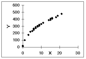
A)a log x transform may be useful
B)a log y transform may be useful
C)a x2 transform may be useful
D)no transform is needed
E)a 1/y transform may be useful
A)a log x transform may be useful
B)a log y transform may be useful
C)a x2 transform may be useful
D)no transform is needed
E)a 1/y transform may be useful
سؤال
سؤال
سؤال
سؤال
سؤال
سؤال
سؤال
The following scatter plot indicates that _________. 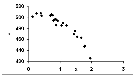
A)a log x transform may be useful
B)a log y transform may be useful
C)an x2 transform may be useful
D)no transform is needed
E)a (- x)transform may be useful
A)a log x transform may be useful
B)a log y transform may be useful
C)an x2 transform may be useful
D)no transform is needed
E)a (- x)transform may be useful
سؤال
The following scatter plot indicates that _________. 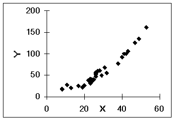
A)a log x transform may be useful
B)a y2 transform may be useful
C)a x2 transform may be useful
D)no transform is needed
E)a 1/x transform may be useful
A)a log x transform may be useful
B)a y2 transform may be useful
C)a x2 transform may be useful
D)no transform is needed
E)a 1/x transform may be useful
سؤال
سؤال
سؤال
سؤال
سؤال
A multiple regression analysis produced the following tables. The regression equation for this analysis is ____________.
A) = 762.1533 + 96.8433 x1 + 3.007943 x12
B)11efcd21_6411_aee5_b057_4518c9fddc20_TB7041_00 = 1411.876 + 762.1533 x1 + 1.852483 x12
C)11efcd21_6411_aee5_b057_4518c9fddc20_TB7041_00 = 1411.876 + 35.18215 x1 + 7.721648 x12
D)11efcd21_6411_aee5_b057_4518c9fddc20_TB7041_00 = 762.1533 + 1.852483 x1 + 0.074919 x12
E)11efcd21_6411_aee5_b057_4518c9fddc20_TB7041_00 = 762.1533 - 1.852483 x1 + 0.074919 x12
A)
= 762.1533 + 96.8433 x1 + 3.007943 x12B)11efcd21_6411_aee5_b057_4518c9fddc20_TB7041_00 = 1411.876 + 762.1533 x1 + 1.852483 x12
C)11efcd21_6411_aee5_b057_4518c9fddc20_TB7041_00 = 1411.876 + 35.18215 x1 + 7.721648 x12
D)11efcd21_6411_aee5_b057_4518c9fddc20_TB7041_00 = 762.1533 + 1.852483 x1 + 0.074919 x12
E)11efcd21_6411_aee5_b057_4518c9fddc20_TB7041_00 = 762.1533 - 1.852483 x1 + 0.074919 x12
سؤال
سؤال
The following scatter plot indicates that _________. 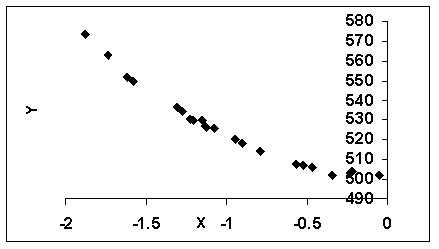
A)a x2 transform may be useful
B)a log y transform may be useful
C)a x4 transform may be useful
D)no transform is needed
E)a x3 transform may be useful
A)a x2 transform may be useful
B)a log y transform may be useful
C)a x4 transform may be useful
D)no transform is needed
E)a x3 transform may be useful
سؤال
سؤال
A local parent group was concerned with the increasing cost of school for families with school aged children.The parent group was interested in understanding the relationship between the academic grade level for the child and the total costs spent per child per academic year.They performed a multiple regression analysis using total cost as the dependent variable and academic year (x1)as the independent variables.The multiple regression analysis produced the following tables. The regression equation for this analysis is ____________.
A)= 707.9144 + 2.903307 x1 + 11.91297 x12
B)11efcd21_6411_aee5_b057_4518c9fddc20_TB7041_00= 707.9144 + 435.1183 x1 + 1.626947 x12
C)11efcd21_6411_aee5_b057_4518c9fddc20_TB7041_00 = 435.1183 + 81.62802 x1 + 3.806211 x12
D)11efcd21_6411_aee5_b057_4518c9fddc20_TB7041_00 = 1.626947 + 0.035568 x1 + 3.129878 x12
E)11efcd21_6411_aee5_b057_4518c9fddc20_TB7041_00 = 1.626947 + 0.035568 x1 - 3.129878 x12
A)
= 707.9144 + 2.903307 x1 + 11.91297 x12B)11efcd21_6411_aee5_b057_4518c9fddc20_TB7041_00= 707.9144 + 435.1183 x1 + 1.626947 x12
C)11efcd21_6411_aee5_b057_4518c9fddc20_TB7041_00 = 435.1183 + 81.62802 x1 + 3.806211 x12
D)11efcd21_6411_aee5_b057_4518c9fddc20_TB7041_00 = 1.626947 + 0.035568 x1 + 3.129878 x12
E)11efcd21_6411_aee5_b057_4518c9fddc20_TB7041_00 = 1.626947 + 0.035568 x1 - 3.129878 x12
سؤال
سؤال
سؤال
سؤال
سؤال
سؤال
سؤال
سؤال
سؤال
سؤال
سؤال
سؤال
سؤال
سؤال
سؤال
سؤال
سؤال
سؤال
Alan Bissell, a market analyst for City Sound Online Mart, is analyzing sales from heavy metal song downloads.Alan's dependent variable is annual heavy metal song download sales (in $1,000,000's), and his independent variables are website visitors (in 1,000's)and type of download format requested (0 = MP3, 1 = other).Regression analysis of the data yielded the following tables. Alan's model is ________________.
A) = 1.7 + 0.384212 x1 + 4.424638 x2 + 0.00166 x3
B)11efcd21_6411_aee5_b057_4518c9fddc20_TB7041_00 = 1.7 + 0.04 x1 + 1.5666667 x2
C)11efcd21_6411_aee5_b057_4518c9fddc20_TB7041_00 = 0.384212 + 0.014029 x1 + 0.20518 x2
D)11efcd21_6411_aee5_b057_4518c9fddc20_TB7041_00 = 4.424638 + 2.851146 x1 - 7.63558 x2
E)11efcd21_6411_aee5_b057_4518c9fddc20_TB7041_00 = 1.7 + 0.04 x1 - 1.5666667 x2
A)
= 1.7 + 0.384212 x1 + 4.424638 x2 + 0.00166 x3B)11efcd21_6411_aee5_b057_4518c9fddc20_TB7041_00 = 1.7 + 0.04 x1 + 1.5666667 x2
C)11efcd21_6411_aee5_b057_4518c9fddc20_TB7041_00 = 0.384212 + 0.014029 x1 + 0.20518 x2
D)11efcd21_6411_aee5_b057_4518c9fddc20_TB7041_00 = 4.424638 + 2.851146 x1 - 7.63558 x2
E)11efcd21_6411_aee5_b057_4518c9fddc20_TB7041_00 = 1.7 + 0.04 x1 - 1.5666667 x2
سؤال
Abby Kratz, a market specialist at the market research firm of Saez, Sikes, and Spitz, is analyzing household budget data collected by her firm.Abby's dependent variable is weekly household expenditures on groceries (in $'s), and her independent variables are annual household income (in $1,000's)and household neighborhood (0 = suburban, 1 = rural).Regression analysis of the data yielded the following table.
Abby's model is ________________.
A)s), and her independent variables are annual household income (in $1,000's)and household neighborhood (0 = suburban, 1 = rural).Regression analysis of the data yielded the following table. \begin{array}{c} \begin{array}{|l|} \hline \text { } \\ \hline \text {Intercept}\\ \hline \text { X_{1} (income)}\\ \hline \text { }\\ \text {(neighborhood)}\\ \hline \end{array} \begin{array}{l} \hline \text { Coefficients }\\ \hline 19.68247 \\ \hline 1.735272 \\ \hline 49.12456\\ \\ \hline \end{array} \begin{array}{|l|} \hline \text {Standard Error}\\ \hline10.01176 \\ \hline 0.174564 \\ \hline 7.655776\\ \\ \hline \end{array} \begin{array}{l|} \hline t \text { Statistic } \\ \hline 1.965934 \\ \hline 9.940612 \\ \hline 6.416667 \\ \\ \hline \end{array} \begin{array}{l|} \hline p \text {-value }\\ \hline0.077667\\ \hline1.68 \mathrm{E}-06\\ \hline7.67 \mathrm{E}-05\\ \\ \hline \end{array} \end{array} Abby's model is ________________. A) = 19.68247 + 10.01176 x1 + 1.965934 x2 B) = 1.965934 + 9.940612 x1 + 6.416667 x2 C) = 10.01176 + 0.174564 x1 + 7.655776 x2 D) = 19.68247 - 1.735272 x1 + 49.12456 x2 E) = 19.68247 + 1.735272 x1 + 49.12456 x2
Abby's model is ________________.
A)
" class="answers-bank-image d-block" loading="lazy" > = 19.68247 + 10.01176 x1 + 1.965934 x2
B)11efcd21_6411_aee5_b057_4518c9fddc20_TB7041_00= 1.965934 + 9.940612 x1 + 6.416667 x2
C)11efcd21_6411_aee5_b057_4518c9fddc20_TB7041_00= 10.01176 + 0.174564 x1 + 7.655776 x2
D)11efcd21_6411_aee5_b057_4518c9fddc20_TB7041_00= 19.68247 - 1.735272 x1 + 49.12456 x2
E)11efcd21_6411_aee5_b057_4518c9fddc20_TB7041_00 = 19.68247 + 1.735272 x1 + 49.12456 x2
سؤال
سؤال
سؤال
سؤال
سؤال
سؤال
سؤال
سؤال
سؤال
سؤال
سؤال
سؤال
سؤال
سؤال
سؤال
سؤال
سؤال
سؤال
سؤال
سؤال
سؤال

فتح الحزمة
قم بالتسجيل لفتح البطاقات في هذه المجموعة!
Unlock Deck
Unlock Deck
1/100
العب
ملء الشاشة (f)
Deck 14: Building Multiple Regression Models
1
Stepwise regression is one of the ways to prevent the problem of multicollinearity.
True
2
A linear regression model cannot be used to explore the possibility that a quadratic relationship may exist between two variables.
False
3
The regression model y = 0 + 1 x1 + 2 x2 + 3 x1x2 + is a first order model.
False
4
If a data set contains k independent variables, the "all possible regression" search procedure will determine 2k different models.
فتح الحزمة
افتح القفل للوصول البطاقات البالغ عددها 100 في هذه المجموعة.
فتح الحزمة
k this deck
5
Recoding data cannot improve the fit of a regression model.
فتح الحزمة
افتح القفل للوصول البطاقات البالغ عددها 100 في هذه المجموعة.
فتح الحزمة
k this deck
6
If each pair of independent variables is weakly correlated, there is no problem of multicollinearity.
فتح الحزمة
افتح القفل للوصول البطاقات البالغ عددها 100 في هذه المجموعة.
فتح الحزمة
k this deck
7
If two or more independent variables are highly correlated, the regression analysis is unlikely to suffer from the problem of multicollinearity.
فتح الحزمة
افتح القفل للوصول البطاقات البالغ عددها 100 في هذه المجموعة.
فتح الحزمة
k this deck
8
Regression models in which the highest power of any predictor variable is 1 and in which there are no cross product terms are referred to as first-order models.
فتح الحزمة
افتح القفل للوصول البطاقات البالغ عددها 100 في هذه المجموعة.
فتح الحزمة
k this deck
9
If the effect of an independent variable (e.g., square footage)on a dependent variable (e.g., price)is affected by different ranges of values for a second independent variable (e.g., age ), the two independent variables are said to interact.
فتح الحزمة
افتح القفل للوصول البطاقات البالغ عددها 100 في هذه المجموعة.
فتح الحزمة
k this deck
10
A linear regression model can be used to explore the possibility that a quadratic relationship may exist between two variables by suitably transforming the independent variable.
فتح الحزمة
افتح القفل للوصول البطاقات البالغ عددها 100 في هذه المجموعة.
فتح الحزمة
k this deck
11
A qualitative variable which represents categories such as geographical territories or job classifications may be included in a regression model by using indicator or dummy variables.
فتح الحزمة
افتح القفل للوصول البطاقات البالغ عددها 100 في هذه المجموعة.
فتح الحزمة
k this deck
12
A logarithmic transformation may be applied to both positive and negative numbers.
فتح الحزمة
افتح القفل للوصول البطاقات البالغ عددها 100 في هذه المجموعة.
فتح الحزمة
k this deck
13
If a qualitative variable has c categories, then only (c - 1)dummy variables must be included in the regression model.
فتح الحزمة
افتح القفل للوصول البطاقات البالغ عددها 100 في هذه المجموعة.
فتح الحزمة
k this deck
14
If a square-transformation is applied to a series of positive numbers, all greater than 1, the numerical values of the numbers in the transformed series will be smaller than the corresponding numbers in the original series.
فتح الحزمة
افتح القفل للوصول البطاقات البالغ عددها 100 في هذه المجموعة.
فتح الحزمة
k this deck
15
The regression model y = 0 + 1 x1 + 2 x21 + is called a quadratic model.
فتح الحزمة
افتح القفل للوصول البطاقات البالغ عددها 100 في هذه المجموعة.
فتح الحزمة
k this deck
16
Qualitative data can be incorporated into linear regression models using indicator variables.
فتح الحزمة
افتح القفل للوصول البطاقات البالغ عددها 100 في هذه المجموعة.
فتح الحزمة
k this deck
17
If a data set contains k independent variables, the "all possible regression" search procedure will determine 2k - 1 different models.
فتح الحزمة
افتح القفل للوصول البطاقات البالغ عددها 100 في هذه المجموعة.
فتح الحزمة
k this deck
18
If a qualitative variable has c categories, then c dummy variables must be included in the regression model, one for each category.
فتح الحزمة
افتح القفل للوصول البطاقات البالغ عددها 100 في هذه المجموعة.
فتح الحزمة
k this deck
19
The interaction between two independent variables can be examined by including a new variable, which is the sum of the two independent variables, in the regression model.
فتح الحزمة
افتح القفل للوصول البطاقات البالغ عددها 100 في هذه المجموعة.
فتح الحزمة
k this deck
20
The regression model y = 0 + 1 x1 + 2 x2 + 3 x3 + is a third order model.
فتح الحزمة
افتح القفل للوصول البطاقات البالغ عددها 100 في هذه المجموعة.
فتح الحزمة
k this deck
21
We may use logistic regression when the dependent variable is a dummy variable, coded 0 or 1.
فتح الحزمة
افتح القفل للوصول البطاقات البالغ عددها 100 في هذه المجموعة.
فتح الحزمة
k this deck
22
Multiple linear regression models can handle certain nonlinear relationships by ________.
A)biasing the sample
B)recoding or transforming variables
C)adjusting the resultant ANOVA table
D)adjusting the observed t and F values
E)performing nonlinear regression
A)biasing the sample
B)recoding or transforming variables
C)adjusting the resultant ANOVA table
D)adjusting the observed t and F values
E)performing nonlinear regression
فتح الحزمة
افتح القفل للوصول البطاقات البالغ عددها 100 في هذه المجموعة.
فتح الحزمة
k this deck
23
The following scatter plot indicates that _________.
A)a log x transform may be useful
B)a log y transform may be useful
C)a x2 transform may be useful
D)no transform is needed
E)a 1/y transform may be useful
A)a log x transform may be useful
B)a log y transform may be useful
C)a x2 transform may be useful
D)no transform is needed
E)a 1/y transform may be useful
فتح الحزمة
افتح القفل للوصول البطاقات البالغ عددها 100 في هذه المجموعة.
فتح الحزمة
k this deck
24
A multiple regression analysis produced the following tables. The sample size for this analysis is ____________.
A)28
B)25
C)30
D)27
E)2
A)28
B)25
C)30
D)27
E)2
فتح الحزمة
افتح القفل للوصول البطاقات البالغ عددها 100 في هذه المجموعة.
فتح الحزمة
k this deck
25
If the variance inflation factor is bigger than 10, the regression analysis might suffer from the problem of multicollinearity.
فتح الحزمة
افتح القفل للوصول البطاقات البالغ عددها 100 في هذه المجموعة.
فتح الحزمة
k this deck
26
To test the overall effectiveness of a logistic regression, a chi-squared statistic is used.
فتح الحزمة
افتح القفل للوصول البطاقات البالغ عددها 100 في هذه المجموعة.
فتح الحزمة
k this deck
27
When structuring a logistic regression model, only one independent or predictor variable can be used.
فتح الحزمة
افتح القفل للوصول البطاقات البالغ عددها 100 في هذه المجموعة.
فتح الحزمة
k this deck
28
A multiple regression analysis produced the following tables. Using = 0.10 to test the null hypothesis H0: 2 = 0, the critical t value is ____.
A)± 1.316
B)± 1.314
C)± 1.703
D)± 1.780
E)± 1.708
A)± 1.316
B)± 1.314
C)± 1.703
D)± 1.780
E)± 1.708
فتح الحزمة
افتح القفل للوصول البطاقات البالغ عددها 100 في هذه المجموعة.
فتح الحزمة
k this deck
29
A multiple regression analysis produced the following tables. Using = 0.10 to test the null hypothesis H0: 1 = 0, the critical t value is ____.
A)± 1.316
B)± 1.314
C)± 1.703
D)± 1.780
E)± 1.708
A)± 1.316
B)± 1.314
C)± 1.703
D)± 1.780
E)± 1.708
فتح الحزمة
افتح القفل للوصول البطاقات البالغ عددها 100 في هذه المجموعة.
فتح الحزمة
k this deck
30
The following scatter plot indicates that _________.
A)a log x transform may be useful
B)a log y transform may be useful
C)an x2 transform may be useful
D)no transform is needed
E)a (- x)transform may be useful
A)a log x transform may be useful
B)a log y transform may be useful
C)an x2 transform may be useful
D)no transform is needed
E)a (- x)transform may be useful
فتح الحزمة
افتح القفل للوصول البطاقات البالغ عددها 100 في هذه المجموعة.
فتح الحزمة
k this deck
31
The following scatter plot indicates that _________.
A)a log x transform may be useful
B)a y2 transform may be useful
C)a x2 transform may be useful
D)no transform is needed
E)a 1/x transform may be useful
A)a log x transform may be useful
B)a y2 transform may be useful
C)a x2 transform may be useful
D)no transform is needed
E)a 1/x transform may be useful
فتح الحزمة
افتح القفل للوصول البطاقات البالغ عددها 100 في هذه المجموعة.
فتح الحزمة
k this deck
32
A local parent group was concerned with the increasing cost of school for families with school aged children.The parent group was interested in understanding the relationship between the academic grade level for the child and the total costs spent per child per academic year.They performed a multiple regression analysis using total cost as the dependent variable and academic year (x1)as the independent variables.The multiple regression analysis produced the following tables. The sample size for this analysis is ____________.
A)27
B)29
C)30
D)25
E)28
A)27
B)29
C)30
D)25
E)28
فتح الحزمة
افتح القفل للوصول البطاقات البالغ عددها 100 في هذه المجموعة.
فتح الحزمة
k this deck
33
The logistic regression model constrains the estimated probabilities to lie between 0 and 100.
فتح الحزمة
افتح القفل للوصول البطاقات البالغ عددها 100 في هذه المجموعة.
فتح الحزمة
k this deck
34
A multiple regression analysis produced the following tables. Using = 0.05 to test the null hypothesis H0: 1 = 2 = 0, the critical F value is ____.
A)4.24
B)3.39
C)5.57
D)3.35
E)2.35
A)4.24
B)3.39
C)5.57
D)3.35
E)2.35
فتح الحزمة
افتح القفل للوصول البطاقات البالغ عددها 100 في هذه المجموعة.
فتح الحزمة
k this deck
35
A multiple regression analysis produced the following tables. For x1= 20, the predicted value of y is ____________.
A)5,204.18.
B)2,031.38
C)2,538.86
D)6262.19
E)6,535.86
A)5,204.18.
B)2,031.38
C)2,538.86
D)6262.19
E)6,535.86
فتح الحزمة
افتح القفل للوصول البطاقات البالغ عددها 100 في هذه المجموعة.
فتح الحزمة
k this deck
36
A multiple regression analysis produced the following tables. The regression equation for this analysis is ____________.
A) = 762.1533 + 96.8433 x1 + 3.007943 x12
B)11efcd21_6411_aee5_b057_4518c9fddc20_TB7041_00 = 1411.876 + 762.1533 x1 + 1.852483 x12
C)11efcd21_6411_aee5_b057_4518c9fddc20_TB7041_00 = 1411.876 + 35.18215 x1 + 7.721648 x12
D)11efcd21_6411_aee5_b057_4518c9fddc20_TB7041_00 = 762.1533 + 1.852483 x1 + 0.074919 x12
E)11efcd21_6411_aee5_b057_4518c9fddc20_TB7041_00 = 762.1533 - 1.852483 x1 + 0.074919 x12
A)
= 762.1533 + 96.8433 x1 + 3.007943 x12B)11efcd21_6411_aee5_b057_4518c9fddc20_TB7041_00 = 1411.876 + 762.1533 x1 + 1.852483 x12
C)11efcd21_6411_aee5_b057_4518c9fddc20_TB7041_00 = 1411.876 + 35.18215 x1 + 7.721648 x12
D)11efcd21_6411_aee5_b057_4518c9fddc20_TB7041_00 = 762.1533 + 1.852483 x1 + 0.074919 x12
E)11efcd21_6411_aee5_b057_4518c9fddc20_TB7041_00 = 762.1533 - 1.852483 x1 + 0.074919 x12
فتح الحزمة
افتح القفل للوصول البطاقات البالغ عددها 100 في هذه المجموعة.
فتح الحزمة
k this deck
37
A multiple regression analysis produced the following tables. For x1= 10, the predicted value of y is ____________.
A)8.88.
B)2,031.38
C)2,53.86
D)262.19
E)2,535.86
A)8.88.
B)2,031.38
C)2,53.86
D)262.19
E)2,535.86
فتح الحزمة
افتح القفل للوصول البطاقات البالغ عددها 100 في هذه المجموعة.
فتح الحزمة
k this deck
38
The following scatter plot indicates that _________.
A)a x2 transform may be useful
B)a log y transform may be useful
C)a x4 transform may be useful
D)no transform is needed
E)a x3 transform may be useful
A)a x2 transform may be useful
B)a log y transform may be useful
C)a x4 transform may be useful
D)no transform is needed
E)a x3 transform may be useful
فتح الحزمة
افتح القفل للوصول البطاقات البالغ عددها 100 في هذه المجموعة.
فتح الحزمة
k this deck
39
A local parent group was concerned with the increasing cost of school for families with school aged children.The parent group was interested in understanding the relationship between the academic grade level for the child and the total costs spent per child per academic year.They performed a multiple regression analysis using total cost as the dependent variable and academic year (x1)as the independent variables.The multiple regression analysis produced the following tables. Using = 0.01 to test the null hypothesis H0: 1 = 2 = 0, the critical F value is ____.
A)5.42
B)5.49
C)7.60
D)3.35
E)2.49
A)5.42
B)5.49
C)7.60
D)3.35
E)2.49
فتح الحزمة
افتح القفل للوصول البطاقات البالغ عددها 100 في هذه المجموعة.
فتح الحزمة
k this deck
40
A local parent group was concerned with the increasing cost of school for families with school aged children.The parent group was interested in understanding the relationship between the academic grade level for the child and the total costs spent per child per academic year.They performed a multiple regression analysis using total cost as the dependent variable and academic year (x1)as the independent variables.The multiple regression analysis produced the following tables. The regression equation for this analysis is ____________.
A)= 707.9144 + 2.903307 x1 + 11.91297 x12
B)11efcd21_6411_aee5_b057_4518c9fddc20_TB7041_00= 707.9144 + 435.1183 x1 + 1.626947 x12
C)11efcd21_6411_aee5_b057_4518c9fddc20_TB7041_00 = 435.1183 + 81.62802 x1 + 3.806211 x12
D)11efcd21_6411_aee5_b057_4518c9fddc20_TB7041_00 = 1.626947 + 0.035568 x1 + 3.129878 x12
E)11efcd21_6411_aee5_b057_4518c9fddc20_TB7041_00 = 1.626947 + 0.035568 x1 - 3.129878 x12
A)
= 707.9144 + 2.903307 x1 + 11.91297 x12B)11efcd21_6411_aee5_b057_4518c9fddc20_TB7041_00= 707.9144 + 435.1183 x1 + 1.626947 x12
C)11efcd21_6411_aee5_b057_4518c9fddc20_TB7041_00 = 435.1183 + 81.62802 x1 + 3.806211 x12
D)11efcd21_6411_aee5_b057_4518c9fddc20_TB7041_00 = 1.626947 + 0.035568 x1 + 3.129878 x12
E)11efcd21_6411_aee5_b057_4518c9fddc20_TB7041_00 = 1.626947 + 0.035568 x1 - 3.129878 x12
فتح الحزمة
افتح القفل للوصول البطاقات البالغ عددها 100 في هذه المجموعة.
فتح الحزمة
k this deck
41
After a transformation of the y-variable values into log y, and performing a regression analysis produced the following tables. For x1= 10, the predicted value of y is ____________.
A)155.79
B)1.25
C)2.42
D)189.06
E)18.90
A)155.79
B)1.25
C)2.42
D)189.06
E)18.90
فتح الحزمة
افتح القفل للوصول البطاقات البالغ عددها 100 في هذه المجموعة.
فتح الحزمة
k this deck
42
In multiple regression analysis, qualitative variables are sometimes referred to as ___.
A)dummy variables
B)quantitative variables
C)dependent variables
D)performance variables
E)cardinal variables
A)dummy variables
B)quantitative variables
C)dependent variables
D)performance variables
E)cardinal variables
فتح الحزمة
افتح القفل للوصول البطاقات البالغ عددها 100 في هذه المجموعة.
فتح الحزمة
k this deck
43
A local parent group was concerned with the increasing cost of school for families with school aged children.The parent group was interested in understanding the relationship between the academic grade level for the child and the total costs spent per child per academic year.They performed a multiple regression analysis using total cost as the dependent variable and academic year (x1)as the independent variables.The multiple regression analysis produced the following tables. Using = 0.05 to test the null hypothesis H0: 1 = 0, the critical t value is ____.
A)± 1.311
B)± 1.699
C)± 1.703
D)± 2.502
E)± 2.052
A)± 1.311
B)± 1.699
C)± 1.703
D)± 2.502
E)± 2.052
فتح الحزمة
افتح القفل للوصول البطاقات البالغ عددها 100 في هذه المجموعة.
فتح الحزمة
k this deck
44
Yvonne Yang, VP of Finance at Discrete Components, Inc.(DCI), wants a regression model which predicts the average collection period on credit sales.Her data set includes two qualitative variables: sales discount rates (0%, 2%, 4%, and 6%), and total assets of credit customers (small, medium, and large).The number of dummy variables needed for "total assets of credit customer" in Yvonne's regression model is ________.
A)1
B)2
C)3
D)4
E)7
A)1
B)2
C)3
D)4
E)7
فتح الحزمة
افتح القفل للوصول البطاقات البالغ عددها 100 في هذه المجموعة.
فتح الحزمة
k this deck
45
Hope Hernandez is the new regional Vice President for a large gasoline station chain.She wants a regression model to predict sales in the convenience stores.Her data set includes two qualitative variables: the gasoline station location (inner city, freeway, and suburbs), and curb appeal of the convenience store (low, medium, and high).The number of dummy variables needed for "curb appeal" in Hope's regression model is ______.
A)1
B)2
C)3
D)4
E)5
A)1
B)2
C)3
D)4
E)5
فتح الحزمة
افتح القفل للوصول البطاقات البالغ عددها 100 في هذه المجموعة.
فتح الحزمة
k this deck
46
Abby Kratz, a market specialist at the market research firm of Saez, Sikes, and Spitz, is analyzing household budget data collected by her firm.Abby's dependent variable is weekly household expenditures on groceries (in $'s), and her independent variables are annual household income (in $1,000's)and household neighborhood (0 = suburban, 1 = rural).Regression analysis of the data yielded the following table. For two households, one suburban and one rural, Abby's model predicts ________.
A)equal weekly expenditures for groceries
B)the suburban household's weekly expenditures for groceries will be $49 more
C)the rural household's weekly expenditures for groceries will be $49 more
D)the suburban household's weekly expenditures for groceries will be $8 more
E)the rural household's weekly expenditures for groceries will be $49 less
فتح الحزمة
افتح القفل للوصول البطاقات البالغ عددها 100 في هذه المجموعة.
فتح الحزمة
k this deck
47
A local parent group was concerned with the increasing cost of school for families with school aged children.The parent group was interested in understanding the relationship between the academic grade level for the child and the total costs spent per child per academic year.They performed a multiple regression analysis using total cost as the dependent variable and academic year (x1)as the independent variables.The multiple regression analysis produced the following tables. For a child in grade 10 (x1= 10)the predicted value of y is ____________.
A)707.91
B)1,117.38
C)856.08
D)2,189.54
E)1,928.24
A)707.91
B)1,117.38
C)856.08
D)2,189.54
E)1,928.24
فتح الحزمة
افتح القفل للوصول البطاقات البالغ عددها 100 في هذه المجموعة.
فتح الحزمة
k this deck
48
Alan Bissell, a market analyst for City Sound Online Mart, is analyzing sales from heavy metal song downloads.Alan's dependent variable is annual heavy metal song download sales (in $1,000,000's), and his independent variables are website visitors (in 1,000's)and type of download format requested (0 = MP3, 1 = other).Regression analysis of the data yielded the following tables. For the same number of website visitors, what is difference between the predicted sales for MP3 versus 'other' heavy metal song downloads
A)$1,566,666 higher sales for 'other' formats
B)the same sales for both formats
C)$1,566,666 lower sales for the 'other' format
D)$1,700,000 higher sales for the MP3 format
E)$ 1,700,000 lower sales for the 'other' format
A)$1,566,666 higher sales for 'other' formats
B)the same sales for both formats
C)$1,566,666 lower sales for the 'other' format
D)$1,700,000 higher sales for the MP3 format
E)$ 1,700,000 lower sales for the 'other' format
فتح الحزمة
افتح القفل للوصول البطاقات البالغ عددها 100 في هذه المجموعة.
فتح الحزمة
k this deck
49
Yvonne Yang, VP of Finance at Discrete Components, Inc.(DCI), wants a regression model which predicts the average collection period on credit sales.Her data set includes two qualitative variables: sales discount rates (0%, 2%, 4%, and 6%), and total assets of credit customers (small, medium, and large).The number of dummy variables needed for "sales discount rate" in Yvonne's regression model is ________.
A)1
B)2
C)3
D)4
E)7
A)1
B)2
C)3
D)4
E)7
فتح الحزمة
افتح القفل للوصول البطاقات البالغ عددها 100 في هذه المجموعة.
فتح الحزمة
k this deck
50
If a qualitative variable has 4 categories, how many dummy variables must be created and used in the regression analysis?
A)3
B)4
C)5
D)6
E)7
A)3
B)4
C)5
D)6
E)7
فتح الحزمة
افتح القفل للوصول البطاقات البالغ عددها 100 في هذه المجموعة.
فتح الحزمة
k this deck
51
Hope Hernandez is the new regional Vice President for a large gasoline station chain.She wants a regression model to predict sales in the convenience stores.Her data set includes two qualitative variables: the gasoline station location (inner city, freeway, and suburbs), and curb appeal of the convenience store (low, medium, and high).The number of dummy variables needed for Hope's regression model is ______.
A)2
B)4
C)6
D)8
E)9
A)2
B)4
C)6
D)8
E)9
فتح الحزمة
افتح القفل للوصول البطاقات البالغ عددها 100 في هذه المجموعة.
فتح الحزمة
k this deck
52
Abby Kratz, a market specialist at the market research firm of Saez, Sikes, and Spitz, is analyzing household budget data collected by her firm.Abby's dependent variable is weekly household expenditures on groceries (in $'s), and her independent variables are annual household income (in $1,000's)and household neighborhood (0 = suburban, 1 = rural).Regression analysis of the data yielded the following table. For a rural household with $90,000 annual income, Abby's model predicts weekly grocery expenditure of ________________.
A)$156.19
B)$224.98
C)$444.62
D)$141.36
E)$175.86
A)$156.19
B)$224.98
C)$444.62
D)$141.36
E)$175.86
فتح الحزمة
افتح القفل للوصول البطاقات البالغ عددها 100 في هذه المجموعة.
فتح الحزمة
k this deck
53
A local parent group was concerned with the increasing cost of school for families with school aged children.The parent group was interested in understanding the relationship between the academic grade level for the child and the total costs spent per child per academic year.They performed a multiple regression analysis using total cost as the dependent variable and academic year (x1)as the independent variables.The multiple regression analysis produced the following tables. For a child in grade 5 (x1= 5), the predicted value of y is ____________.
A)707.91
B)1,020.26
C)781.99
D)840.06
E)1078.32
A)707.91
B)1,020.26
C)781.99
D)840.06
E)1078.32
فتح الحزمة
افتح القفل للوصول البطاقات البالغ عددها 100 في هذه المجموعة.
فتح الحزمة
k this deck
54
A local parent group was concerned with the increasing cost of school for families with school aged children.The parent group was interested in understanding the relationship between the academic grade level for the child and the total costs spent per child per academic year.They performed a multiple regression analysis using total cost as the dependent variable and academic year (x1)as the independent variables.The multiple regression analysis produced the following tables. These results indicate that ____________.
A)none of the predictor variables is significant at the 5% level
B)each predictor variable is significant at the 5% level
C)x1 is the only predictor variable significant at the 5% level
D)x12 is the only predictor variable significant at the 5% level
E)each predictor variable is insignificant at the 5% level
فتح الحزمة
افتح القفل للوصول البطاقات البالغ عددها 100 في هذه المجموعة.
فتح الحزمة
k this deck
55
Alan Bissell, a market analyst for City Sound Online Mart, is analyzing sales from heavy metal song downloads.Alan's dependent variable is annual heavy metal song download sales (in $1,000,000's), and his independent variables are website visitors (in 1,000's)and type of download format requested (0 = MP3, 1 = other).Regression analysis of the data yielded the following tables. For 'other' download formats with 10,000 website visitors, Alan's model predicts annual sales of heavy metal song downloads of ________________.
A)$2,100,000
B)$524,507
C)$533,333
D)$729,683
E)$210,000
A)$2,100,000
B)$524,507
C)$533,333
D)$729,683
E)$210,000
فتح الحزمة
افتح القفل للوصول البطاقات البالغ عددها 100 في هذه المجموعة.
فتح الحزمة
k this deck
56
Alan Bissell, a market analyst for City Sound Online Mart, is analyzing sales from heavy metal song downloads.Alan's dependent variable is annual heavy metal song download sales (in $1,000,000's), and his independent variables are website visitors (in 1,000's)and type of download format requested (0 = MP3, 1 = other).Regression analysis of the data yielded the following tables. For MP3 sales with 10,000 website visitors, Alan's model predicts annual sales of heavy metal song downloads of ________________.
A)$2,100,000
B)$524,507
C)$533,333
D)$729,683
E)$21,000,000
A)$2,100,000
B)$524,507
C)$533,333
D)$729,683
E)$21,000,000
فتح الحزمة
افتح القفل للوصول البطاقات البالغ عددها 100 في هذه المجموعة.
فتح الحزمة
k this deck
57
Abby Kratz, a market specialist at the market research firm of Saez, Sikes, and Spitz, is analyzing household budget data collected by her firm.Abby's dependent variable is weekly household expenditures on groceries (in $'s), and her independent variables are annual household income (in $1,000's)and household neighborhood (0 = suburban, 1 = rural).Regression analysis of the data yielded the following table. For a suburban household with $90,000 annual income, Abby's model predicts weekly grocery expenditure of ________________.
A)$156.19
B)$224.98
C)$444.62
D)$141.36
E)$175.86
A)$156.19
B)$224.98
C)$444.62
D)$141.36
E)$175.86
فتح الحزمة
افتح القفل للوصول البطاقات البالغ عددها 100 في هذه المجموعة.
فتح الحزمة
k this deck
58
Alan Bissell, a market analyst for City Sound Online Mart, is analyzing sales from heavy metal song downloads.Alan's dependent variable is annual heavy metal song download sales (in $1,000,000's), and his independent variables are website visitors (in 1,000's)and type of download format requested (0 = MP3, 1 = other).Regression analysis of the data yielded the following tables. Alan's model is ________________.
A) = 1.7 + 0.384212 x1 + 4.424638 x2 + 0.00166 x3
B)11efcd21_6411_aee5_b057_4518c9fddc20_TB7041_00 = 1.7 + 0.04 x1 + 1.5666667 x2
C)11efcd21_6411_aee5_b057_4518c9fddc20_TB7041_00 = 0.384212 + 0.014029 x1 + 0.20518 x2
D)11efcd21_6411_aee5_b057_4518c9fddc20_TB7041_00 = 4.424638 + 2.851146 x1 - 7.63558 x2
E)11efcd21_6411_aee5_b057_4518c9fddc20_TB7041_00 = 1.7 + 0.04 x1 - 1.5666667 x2
A)
= 1.7 + 0.384212 x1 + 4.424638 x2 + 0.00166 x3B)11efcd21_6411_aee5_b057_4518c9fddc20_TB7041_00 = 1.7 + 0.04 x1 + 1.5666667 x2
C)11efcd21_6411_aee5_b057_4518c9fddc20_TB7041_00 = 0.384212 + 0.014029 x1 + 0.20518 x2
D)11efcd21_6411_aee5_b057_4518c9fddc20_TB7041_00 = 4.424638 + 2.851146 x1 - 7.63558 x2
E)11efcd21_6411_aee5_b057_4518c9fddc20_TB7041_00 = 1.7 + 0.04 x1 - 1.5666667 x2
فتح الحزمة
افتح القفل للوصول البطاقات البالغ عددها 100 في هذه المجموعة.
فتح الحزمة
k this deck
59
Abby Kratz, a market specialist at the market research firm of Saez, Sikes, and Spitz, is analyzing household budget data collected by her firm.Abby's dependent variable is weekly household expenditures on groceries (in $'s), and her independent variables are annual household income (in $1,000's)and household neighborhood (0 = suburban, 1 = rural).Regression analysis of the data yielded the following table.
Abby's model is ________________.
A) }\\ \text {(neighborhood)}\\ \hline \end{array} \begin{array}{l} \hline \text { Coefficients }\\ \hline 19.68247 \\ \hline 1.735272 \\ \hline 49.12456\\ \\ \hline \end{array} \begin{array}{|l|} \hline \text {Standard Error}\\ \hline10.01176 \\ \hline 0.174564 \\ \hline 7.655776\\ \\ \hline \end{array} \begin{array}{l|} \hline t \text { Statistic } \\ \hline 1.965934 \\ \hline 9.940612 \\ \hline 6.416667 \\ \\ \hline \end{array} \begin{array}{l|} \hline p \text {-value }\\ \hline0.077667\\ \hline1.68 \mathrm{E}-06\\ \hline7.67 \mathrm{E}-05\\ \\ \hline \end{array} \end{array} Abby's model is ________________. A) = 19.68247 + 10.01176 x1 + 1.965934 x2 B) = 1.965934 + 9.940612 x1 + 6.416667 x2 C) = 10.01176 + 0.174564 x1 + 7.655776 x2 D) = 19.68247 - 1.735272 x1 + 49.12456 x2 E) = 19.68247 + 1.735272 x1 + 49.12456 x2 " class="answers-bank-image d-block" loading="lazy" > = 19.68247 + 10.01176 x1 + 1.965934 x2
B)11efcd21_6411_aee5_b057_4518c9fddc20_TB7041_00= 1.965934 + 9.940612 x1 + 6.416667 x2
C)11efcd21_6411_aee5_b057_4518c9fddc20_TB7041_00= 10.01176 + 0.174564 x1 + 7.655776 x2
D)11efcd21_6411_aee5_b057_4518c9fddc20_TB7041_00= 19.68247 - 1.735272 x1 + 49.12456 x2
E)11efcd21_6411_aee5_b057_4518c9fddc20_TB7041_00 = 19.68247 + 1.735272 x1 + 49.12456 x2
Abby's model is ________________.
A)
}\\ \text {(neighborhood)}\\ \hline \end{array} \begin{array}{l} \hline \text { Coefficients }\\ \hline 19.68247 \\ \hline 1.735272 \\ \hline 49.12456\\ \\ \hline \end{array} \begin{array}{|l|} \hline \text {Standard Error}\\ \hline10.01176 \\ \hline 0.174564 \\ \hline 7.655776\\ \\ \hline \end{array} \begin{array}{l|} \hline t \text { Statistic } \\ \hline 1.965934 \\ \hline 9.940612 \\ \hline 6.416667 \\ \\ \hline \end{array} \begin{array}{l|} \hline p \text {-value }\\ \hline0.077667\\ \hline1.68 \mathrm{E}-06\\ \hline7.67 \mathrm{E}-05\\ \\ \hline \end{array} \end{array} Abby's model is ________________. A) = 19.68247 + 10.01176 x1 + 1.965934 x2 B) = 1.965934 + 9.940612 x1 + 6.416667 x2 C) = 10.01176 + 0.174564 x1 + 7.655776 x2 D) = 19.68247 - 1.735272 x1 + 49.12456 x2 E) = 19.68247 + 1.735272 x1 + 49.12456 x2 " class="answers-bank-image d-block" loading="lazy" > = 19.68247 + 10.01176 x1 + 1.965934 x2B)11efcd21_6411_aee5_b057_4518c9fddc20_TB7041_00= 1.965934 + 9.940612 x1 + 6.416667 x2
C)11efcd21_6411_aee5_b057_4518c9fddc20_TB7041_00= 10.01176 + 0.174564 x1 + 7.655776 x2
D)11efcd21_6411_aee5_b057_4518c9fddc20_TB7041_00= 19.68247 - 1.735272 x1 + 49.12456 x2
E)11efcd21_6411_aee5_b057_4518c9fddc20_TB7041_00 = 19.68247 + 1.735272 x1 + 49.12456 x2
فتح الحزمة
افتح القفل للوصول البطاقات البالغ عددها 100 في هذه المجموعة.
فتح الحزمة
k this deck
60
A local parent group was concerned with the increasing cost of school for families with school aged children.The parent group was interested in understanding the relationship between the academic grade level for the child and the total costs spent per child per academic year.They performed a multiple regression analysis using total cost as the dependent variable and academic year (x1)as the independent variables.The multiple regression analysis produced the following tables. Using = 0.05 to test the null hypothesis H0: 2 = 0, the critical t value is ____.
A)± 1.311
B)± 1.699
C)± 1.703
D)± 2.052
E)± 2.502
A)± 1.311
B)± 1.699
C)± 1.703
D)± 2.052
E)± 2.502
فتح الحزمة
افتح القفل للوصول البطاقات البالغ عددها 100 في هذه المجموعة.
فتح الحزمة
k this deck
61
Inspection of the following table of correlation coefficients for variables in a multiple regression analysis reveals potential multicollinearity with variables ___________.
A)x1 and x2
B)x1 and x4
C)x4 and x5
D)x4 and x3
E)x5 and y
A)x1 and x2
B)x1 and x4
C)x4 and x5
D)x4 and x3
E)x5 and y
فتح الحزمة
افتح القفل للوصول البطاقات البالغ عددها 100 في هذه المجموعة.
فتح الحزمة
k this deck
62
Inspection of the following table of t values for variables in a multiple regression analysis reveals that the first independent variable that will be entered into the regression model by the forward selection procedure will be ___________.
A)x1
B)x2
C)x3
D)x4
E)x5
A)x1
B)x2
C)x3
D)x4
E)x5
فتح الحزمة
افتح القفل للوصول البطاقات البالغ عددها 100 في هذه المجموعة.
فتح الحزمة
k this deck
63
An appropriate method to identify multicollinearity in a regression model is to ____.
A)examine a residual plot
B)examine the ANOVA table
C)examine a correlation matrix
D)examine the partial regression coefficients
E)examine the R2 of the regression model
A)examine a residual plot
B)examine the ANOVA table
C)examine a correlation matrix
D)examine the partial regression coefficients
E)examine the R2 of the regression model
فتح الحزمة
افتح القفل للوصول البطاقات البالغ عددها 100 في هذه المجموعة.
فتح الحزمة
k this deck
64
Which of the following iterative search procedures for model-building in a multiple regression analysis adds variables to model as it proceeds, but does not reevaluate the contribution of previously entered variables?
A)Backward elimination
B)Stepwise regression
C)Forward selection
D)All possible regressions
E)Forward elimination
A)Backward elimination
B)Stepwise regression
C)Forward selection
D)All possible regressions
E)Forward elimination
فتح الحزمة
افتح القفل للوصول البطاقات البالغ عددها 100 في هذه المجموعة.
فتح الحزمة
k this deck
65
Inspection of the following table of t values for variables in a multiple regression analysis reveals that the first independent variable that will be entered into the regression model by the forward selection procedure will be ___________.
A)x1
B)x2
C)x3
D)x4
E)x5
A)x1
B)x2
C)x3
D)x4
E)x5
فتح الحزمة
افتح القفل للوصول البطاقات البالغ عددها 100 في هذه المجموعة.
فتح الحزمة
k this deck
66
Which of the following iterative search procedures for model-building in a multiple regression analysis starts with all independent variables in the model and then drops non-significant independent variables is a step-by-step manner?
A)Backward elimination
B)Stepwise regression
C)Forward selection
D)All possible regressions
E)Backward selection
A)Backward elimination
B)Stepwise regression
C)Forward selection
D)All possible regressions
E)Backward selection
فتح الحزمة
افتح القفل للوصول البطاقات البالغ عددها 100 في هذه المجموعة.
فتح الحزمة
k this deck
67
An acceptable method of managing multicollinearity in a regression model is the ___.
A)use the forward selection procedure
B)use the backward elimination procedure
C)use the forward elimination procedure
D)use the stepwise regression procedure
E)use all possible regressions
A)use the forward selection procedure
B)use the backward elimination procedure
C)use the forward elimination procedure
D)use the stepwise regression procedure
E)use all possible regressions
فتح الحزمة
افتح القفل للوصول البطاقات البالغ عددها 100 في هذه المجموعة.
فتح الحزمة
k this deck
68
An "all possible regressions" search of a data set containing 5 independent variables will produce ______ regressions.
A)31
B)10
C)25
D)32
E)24
A)31
B)10
C)25
D)32
E)24
فتح الحزمة
افتح القفل للوصول البطاقات البالغ عددها 100 في هذه المجموعة.
فتح الحزمة
k this deck
69
Inspection of the following table of t values for variables in a multiple regression analysis reveals that the first independent variable entered by the forward selection procedure will be ___________.
A)x1
B)x2
C)x3
D)x4
E)x5
A)x1
B)x2
C)x3
D)x4
E)x5
فتح الحزمة
افتح القفل للوصول البطاقات البالغ عددها 100 في هذه المجموعة.
فتح الحزمة
k this deck
70
An "all possible regressions" search of a data set containing "k" independent variables will produce __________ regressions.
A)2k -1
B)2k - 1
C)k2 - 1
D)2k - 1
E)2k
A)2k -1
B)2k - 1
C)k2 - 1
D)2k - 1
E)2k
فتح الحزمة
افتح القفل للوصول البطاقات البالغ عددها 100 في هذه المجموعة.
فتح الحزمة
k this deck
71
Carlos Cavazos, Director of Human Resources, is exploring employee absenteeism at the Plano Piano Plant.A multiple regression analysis was performed using the following variables.The results are presented below. Which of the following conclusions can be drawn from the above results?
A)All the independent variables in the regression are significant at 5% level.
B)Commuting distance is a highly significant (<1%)variable in explaining absenteeism.
C)Age of the employees tends to have a very significant (<1%)effect on absenteeism.
D)This model explains a little over 49% of the variability in absenteeism data.
E)A single-parent household employee is expected to be absent fewer days, all other variables held constant, compared to one who is not a single-parent household.
فتح الحزمة
افتح القفل للوصول البطاقات البالغ عددها 100 في هذه المجموعة.
فتح الحزمة
k this deck
72
An "all possible regressions" search of a data set containing 8 independent variables will produce ______ regressions.
A)8
B)15
C)256
D)64
E)255
A)8
B)15
C)256
D)64
E)255
فتح الحزمة
افتح القفل للوصول البطاقات البالغ عددها 100 في هذه المجموعة.
فتح الحزمة
k this deck
73
Suppose a company is interested in understanding the effect of age and sex on the likelihood a customer will purchase a new product.The data analyst intends to run a logistic regression on her data.Which of the following variable(s)will the analyst need to code as 0 or 1 prior to performing the logistic regression analysis?
A)age and gender
B)age and purchase status
C)age
D)purchase status
E)sex and purchase status Gender is no longer considered dichotomous
A)age and gender
B)age and purchase status
C)age
D)purchase status
E)sex and purchase status Gender is no longer considered dichotomous
فتح الحزمة
افتح القفل للوصول البطاقات البالغ عددها 100 في هذه المجموعة.
فتح الحزمة
k this deck
74
Inspection of the following table of t values for variables in a multiple regression analysis reveals that the first independent variable entered by the forward selection procedure will be ___________.
A)x2
B)x3
C)x4
D)x5
E)x1
A)x2
B)x3
C)x4
D)x5
E)x1
فتح الحزمة
افتح القفل للوصول البطاقات البالغ عددها 100 في هذه المجموعة.
فتح الحزمة
k this deck
75
An "all possible regressions" search of a data set containing 7 independent variables will produce ______ regressions.
A)13
B)127
C)48
D)64
E)97
A)13
B)127
C)48
D)64
E)97
فتح الحزمة
افتح القفل للوصول البطاقات البالغ عددها 100 في هذه المجموعة.
فتح الحزمة
k this deck
76
Large correlations between two or more independent variables in a multiple regression model could result in the problem of ________.
A)multicollinearity
B)autocorrelation
C)partial correlation
D)rank correlation
E)non-normality
A)multicollinearity
B)autocorrelation
C)partial correlation
D)rank correlation
E)non-normality
فتح الحزمة
افتح القفل للوصول البطاقات البالغ عددها 100 في هذه المجموعة.
فتح الحزمة
k this deck
77
Which of the following iterative search procedures for model-building in a multiple regression analysis reevaluates the contribution of variables previously include in the model after entering a new independent variable?
A)Backward elimination
B)Stepwise regression
C)Forward selection
D)All possible regressions
E)Backward selection
A)Backward elimination
B)Stepwise regression
C)Forward selection
D)All possible regressions
E)Backward selection
فتح الحزمة
افتح القفل للوصول البطاقات البالغ عددها 100 في هذه المجموعة.
فتح الحزمة
k this deck
78
A useful technique in controlling multicollinearity involves the use of _________.
A)variance inflation factors
B)a backward elimination procedure
C)a forward elimination procedure
D)a forward selection procedure
E)all possible regressions
A)variance inflation factors
B)a backward elimination procedure
C)a forward elimination procedure
D)a forward selection procedure
E)all possible regressions
فتح الحزمة
افتح القفل للوصول البطاقات البالغ عددها 100 في هذه المجموعة.
فتح الحزمة
k this deck
79
Inspection of the following table of correlation coefficients for variables in a multiple regression analysis reveals potential multicollinearity with variables ___________.
A)x1 and x2
B)x1 and x5
C)x3 and x4
D)x2 and x5
E)x3 and x5
A)x1 and x2
B)x1 and x5
C)x3 and x4
D)x2 and x5
E)x3 and x5
فتح الحزمة
افتح القفل للوصول البطاقات البالغ عددها 100 في هذه المجموعة.
فتح الحزمة
k this deck
80
Inspection of the following table of correlation coefficients for variables in a multiple regression analysis reveals potential multicollinearity with variables ___________.
A)x1 and x5
B)x2 and x3
C)x4 and x2
D)x4 and x3
E)x4 and y
A)x1 and x5
B)x2 and x3
C)x4 and x2
D)x4 and x3
E)x4 and y
فتح الحزمة
افتح القفل للوصول البطاقات البالغ عددها 100 في هذه المجموعة.
فتح الحزمة
k this deck
فتح الحزمة
افتح القفل للوصول البطاقات البالغ عددها 100 في هذه المجموعة.


