Deck 20: Model Building
ملء الشاشة (f)
سؤال
سؤال
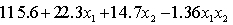
The model  +
+  is referred to as a:
A) first-order model with two predictor variables with no interaction.
B) first-order model with two predictor variables with interaction.
C) second-order model with three predictor variables with no interaction.
D) second-order model with three predictor variables with interaction.
+ is referred to as a:A) first-order model with two predictor variables with no interaction.
B) first-order model with two predictor variables with interaction.
C) second-order model with three predictor variables with no interaction.
D) second-order model with three predictor variables with interaction.
سؤال
سؤال
سؤال
سؤال
The model  +
+  is referred to as a:
A) first-order model with one predictor variable.
B) first-order model with two predictor variables.
C) second-order model with one predictor variable.
D) second-order model with two predictor variables.
+ is referred to as a:A) first-order model with one predictor variable.
B) first-order model with two predictor variables.
C) second-order model with one predictor variable.
D) second-order model with two predictor variables.
سؤال
سؤال
The graph of the model  is shaped like a straight line going upwards.
is shaped like a straight line going upwards. سؤال
سؤال
سؤال
سؤال
Suppose that the sample regression equation of a model is . If we examine the relationship between and y for four different values of , we observe that the four equations produced differ only in the intercept term.
. If we examine the relationship between and y for four different values of , we observe that the four equations produced differ only in the intercept term. سؤال
When we plot x versus y, the graph of the model  +
+  is shaped like a:
A) straight line going upwards.
B) straight line going downwards.
C) circle.
D) parabola.
+ is shaped like a:A) straight line going upwards.
B) straight line going downwards.
C) circle.
D) parabola.
سؤال
سؤال
Suppose that the sample regression line of a first order model is . If we examine the relationship between y and for four different values of , we observe that the:
A) effect of x on y remains the same no matter what the value of x .
B) effect of x on y remains the same no matter what the value of x .
C) only difference in the four equations produced is the coefficient of x .
D) None of these choices are correct.
. If we examine the relationship between y and for four different values of , we observe that the:A) effect of x on y remains the same no matter what the value of x .
B) effect of x on y remains the same no matter what the value of x .
C) only difference in the four equations produced is the coefficient of x .
D) None of these choices are correct.
سؤال
سؤال
For the regression equation , which combination of and , respectively, results in the largest average value of y?
A) 3 and 5.
B) 5 and 3.
C) 6 and 3.
D) 3 and 6.
, which combination of and , respectively, results in the largest average value of y?A) 3 and 5.
B) 5 and 3.
C) 6 and 3.
D) 3 and 6.
سؤال
سؤال
Suppose that the sample regression equation of a model is . If we examine the relationship between and y for three different values of , we observe that the:
A) three equations produced differ only in the intercept.
B) coefficient of remains unchanged.
C) coefficient of varies.
D) three equations produced differ not only in the intercept term but the coefficient of , also varies.
. If we examine the relationship between and y for three different values of , we observe that the:A) three equations produced differ only in the intercept.
B) coefficient of remains unchanged.
C) coefficient of varies.
D) three equations produced differ not only in the intercept term but the coefficient of , also varies.
سؤال
The following model  +
+  is used whenever the statistician believes that, on average, y is linearly related to:
A) , and the predictor variables do not interact.
B) , and the predictor variables do not interact.
C) and the predictor variables do not interact or to
  , and the predictor variables do not interact.
D) and the predictor variables do not interact and to
  , and the predictor variables do not interact.
+ is used whenever the statistician believes that, on average, y is linearly related to:A)
, and the predictor variables do not interact.B)
, and the predictor variables do not interact.C)
and the predictor variables do not interact or to , and the predictor variables do not interact.D)
and the predictor variables do not interact and to , and the predictor variables do not interact. سؤال
سؤال
The model
is referred to as a first-order model with two predictor variables with no interaction.
is referred to as a first-order model with two predictor variables with no interaction.
سؤال
In the first-order model ŷ = 8 + 3x1 +5x2, a unit increase in  , while holding
  constant, increases the value of
  on average by 3 units.
, while holding constant, increases the value of on average by 3 units. سؤال
In the first-order model  = 60 + 40x1 -10x2 + 5x1x2, a unit increase in x1, while holding x2 constant at 1, increases the value of on average by 45 units.
= 60 + 40x1 -10x2 + 5x1x2, a unit increase in x1, while holding x2 constant at 1, increases the value of on average by 45 units. سؤال
In a first-order model with two predictors,  and
and  , an interaction term may be used when the relationship between the dependent variable
  and the predictor variables is linear.
and , an interaction term may be used when the relationship between the dependent variable and the predictor variables is linear. سؤال
سؤال
Suppose that the sample regression line of a first-order model is . If we examine the relationship between y and for three different values of , we observe that the effect of on remains the same no matter what the value of .
. If we examine the relationship between y and for three different values of , we observe that the effect of on remains the same no matter what the value of . سؤال
سؤال
سؤال
سؤال
سؤال
In the first-order model
, a unit increase in , while holding constant at a value of 3, decreases the value of on average by 3 units.
, a unit increase in , while holding constant at a value of 3, decreases the value of on average by 3 units.
سؤال
In the first-order regression model ŷ = 12 + 6x1 +8x2 + 4x1x2, a unit increase in x1 increases the value of  on average by 6 units.
on average by 6 units. سؤال
In the first-order model
, a unit increase in , while holding constant at a value of 2, decreases the value of on average by 8 units.
, a unit increase in , while holding constant at a value of 2, decreases the value of on average by 8 units.
سؤال
Suppose that the sample regression equation of a model is
. If we examine the relationship between y and for = 1, 2 and 3, we observe that the three equations produced not only differ in the intercept term, but the coefficient of also varies.
. If we examine the relationship between y and for = 1, 2 and 3, we observe that the three equations produced not only differ in the intercept term, but the coefficient of also varies.
سؤال
سؤال
The model is used whenever the statistician believes that, on average, is linearly related to and , and the predictor variables do not interact.
is used whenever the statistician believes that, on average, is linearly related to and , and the predictor variables do not interact. سؤال
The model y = 0 + 1x +  is referred to as a simple linear regression model.
is referred to as a simple linear regression model. سؤال
The model y = 0 + 1x + 2x2 + … + pxp + is referred to as a polynomial model with p predictor variables.
is referred to as a polynomial model with p predictor variables. سؤال
The model is referred to as a second-order model with two predictor variables with interaction.
is referred to as a second-order model with two predictor variables with interaction. سؤال
سؤال
Consider the following data for two variables, x and y, where x is the age of a particular make of car
and y is the selling price, in thousands of dollars. Use Excel to test whether the population slope is positive, at the 1% level of significance.
and y is the selling price, in thousands of dollars.
Use Excel to test whether the population slope is positive, at the 1% level of significance. سؤال
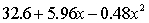
Consider the following data for two variables, x and y. Use the model in  = 66.799 -7.307x + 0.324x2 to predict the value of y when x = 10.
= 66.799 -7.307x + 0.324x2 to predict the value of y when x = 10. سؤال
A regression analysis was performed to study the relationship between a dependent variable and four independent variables. The following information was obtained:
r2 = 0.95, SSR = 9800, n = 50.
ANOVA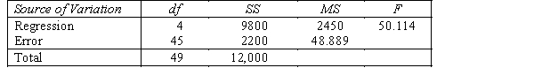 Test the overall validity of the model at the 5% significance level.
r2 = 0.95, SSR = 9800, n = 50.
ANOVA
Test the overall validity of the model at the 5% significance level. سؤال
Consider the following data for two variables, x and y. Use Excel to determine whether there is sufficient evidence at the 1% significance level to infer that the relationship between y, x and in = 66.799 -7.307x + 0.324x2 is significant.
= 66.799 -7.307x + 0.324x2 is significant. سؤال
سؤال
سؤال
Consider the following data for two variables, x and y.  Use Excel to find the coefficient of determination. What does this statistic tell you about this curvilinear model?
Use Excel to find the coefficient of determination. What does this statistic tell you about this curvilinear model? سؤال
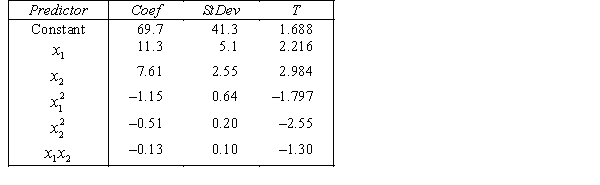
An avid football fan was in the process of examining the factors that determine the success or failure of football teams. He noticed that teams with many rookies and teams with many veterans seem to do quite poorly. To further analyse his beliefs, he took a random sample of 20 teams and proposed a second-order model with one independent variable. The selected model is:  .
.
where
y = winning team's percentage.
x = average years of professional experience.
The computer output is shown below:
THE REGRESSION EQUATION IS:
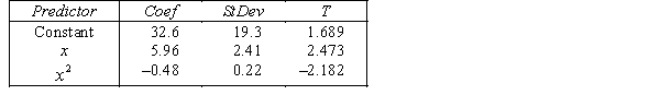 S = 16.1 R-Sq = 43.9%.
ANALYSIS OF VARIANCE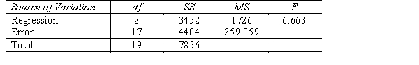 Test to determine at the 10% significance level if the linear term should be retained.
.where
y = winning team's percentage.
x = average years of professional experience.
The computer output is shown below:
THE REGRESSION EQUATION IS:
S = 16.1 R-Sq = 43.9%.ANALYSIS OF VARIANCE
Test to determine at the 10% significance level if the linear term should be retained. سؤال
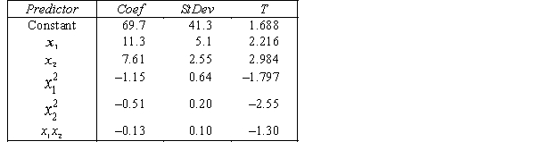
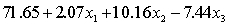
A traffic consultant has analysed the factors that affect the number of traffic fatalities. She has come to the conclusion that two important variables are the number of cars and the number of tractor-trailer trucks. She proposed the second-order model with interaction: 
 .
.
Where:
y = number of annual fatalities per shire. = number of cars registered in the shire (in units of 10 000).
  = number of trucks registered in the shire (in units of 1000).
The computer output (based on a random sample of 35 shires) is shown below.
THE REGRESSION EQUATION IS
 .
.  S = 15.2 R-Sq = 47.2%.
ANALYSIS OF VARIANCE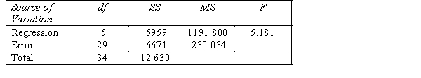 Is there enough evidence at the 5% significance level to conclude that the model is useful in predicting the number of fatalities?
.Where:
y = number of annual fatalities per shire.
= number of cars registered in the shire (in units of 10 000). = number of trucks registered in the shire (in units of 1000).The computer output (based on a random sample of 35 shires) is shown below.
THE REGRESSION EQUATION IS
. S = 15.2 R-Sq = 47.2%.ANALYSIS OF VARIANCE
Is there enough evidence at the 5% significance level to conclude that the model is useful in predicting the number of fatalities? سؤال
سؤال
Consider the following data for two variables, x and y.  Use Excel to find the coefficient of determination. What does this statistic tell you about this simple linear model?
Use Excel to find the coefficient of determination. What does this statistic tell you about this simple linear model? سؤال
سؤال
Consider the following data for two variables, x and y.  Use Excel to develop a scatter diagram for the data. Does the scatter diagram suggest an estimated regression equation of the form ŷ = b0 +b1x + b2x2? Explain.
Use Excel to develop a scatter diagram for the data. Does the scatter diagram suggest an estimated regression equation of the form ŷ = b0 +b1x + b2x2? Explain. سؤال
An avid football fan was in the process of examining the factors that determine the success or failure of football teams. He noticed that teams with many rookies and teams with many veterans seem to do quite poorly. To further analyse his beliefs, he took a random sample of 20 teams and proposed a second-order model with one independent variable. The selected model is: 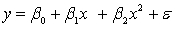 .
.
where
y = winning team's percentage.
x = average years of professional experience.
The computer output is shown below:
THE REGRESSION EQUATION IS:

 S = 16.1 R-Sq = 43.9%.
ANALYSIS OF VARIANCE What is the coefficient of determination? Explain what this statistic tells you about the model.
.where
y = winning team's percentage.
x = average years of professional experience.
The computer output is shown below:
THE REGRESSION EQUATION IS:
S = 16.1 R-Sq = 43.9%.ANALYSIS OF VARIANCE
What is the coefficient of determination? Explain what this statistic tells you about the model. سؤال
سؤال
سؤال
A regression analysis involving 40 observations and five independent variables revealed that the total variation in the dependent variable y is 1080 and that the mean square for error is 30. 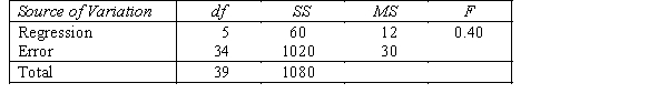 Test the significance of the overall equation at the 5% level of significance.
Test the significance of the overall equation at the 5% level of significance. سؤال
An avid football fan was in the process of examining the factors that determine the success or failure of football teams. He noticed that teams with many rookies and teams with many veterans seem to do quite poorly. To further analyse his beliefs, he took a random sample of 20 teams and proposed a second-order model with one independent variable. The selected model is:  .
.
where
y = winning team's percentage.
x = average years of professional experience.
The computer output is shown below:
THE REGRESSION EQUATION IS:

 S = 16.1 R-Sq = 43.9%.
ANALYSIS OF VARIANCE Test to determine at the 10% significance level whether the
  term should be retained.
.where
y = winning team's percentage.
x = average years of professional experience.
The computer output is shown below:
THE REGRESSION EQUATION IS:
S = 16.1 R-Sq = 43.9%.ANALYSIS OF VARIANCE
Test to determine at the 10% significance level whether the term should be retained. سؤال
Consider the following data for two variables, x and y, where x is the age of a particular make of car
and y is the selling price, in thousands of dollars. a. Use Excel to develop an estimated regression equation of the form = b0 +b1x.
b. Interpret the intercept.
c. Interpret the slope.
and y is the selling price, in thousands of dollars. a. Use Excel to develop an estimated regression equation of the form
= b0 +b1x.b. Interpret the intercept.
c. Interpret the slope.
سؤال
A traffic consultant has analysed the factors that affect the number of traffic fatalities. She has come to the conclusion that two important variables are the number of cars and the number of tractor-trailer trucks. She proposed the second-order model with interaction: 
 .
.
Where:
y = number of annual fatalities per shire. = number of cars registered in the shire (in units of 10 000).
  = number of trucks registered in the shire (in units of 1000).
The computer output (based on a random sample of 35 shires) is shown below.
THE REGRESSION EQUATION IS
 .
.  S = 15.2 R-Sq = 47.2%.
ANALYSIS OF VARIANCE Test at the 1% significance level to determine whether the
  term should be retained in the model.
.Where:
y = number of annual fatalities per shire.
= number of cars registered in the shire (in units of 10 000). = number of trucks registered in the shire (in units of 1000).The computer output (based on a random sample of 35 shires) is shown below.
THE REGRESSION EQUATION IS
. S = 15.2 R-Sq = 47.2%.ANALYSIS OF VARIANCE
Test at the 1% significance level to determine whether the term should be retained in the model. سؤال
An economist is analysing the incomes of professionals (physicians, dentists and lawyers). He realises that an important factor is the number of years of experience. However, he wants to know if there are differences among the three professional groups. He takes a random sample of 125 professionals and estimates the multiple regression model:  .
.
where
y
= annual income (in $1000). = years of experience.
  = 1 if physician.
= 0 if not. = 1 if dentist.
= 0 if not.
The computer output is shown below.
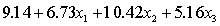
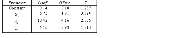
THE REGRESSION EQUATION IS
 .
. 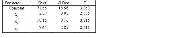 S = 42.6 R-Sq = 30.9%.
  Is there enough evidence at the 5% significance level to conclude that income and experience are linearly related?
.where
y
= annual income (in $1000).
= years of experience. = 1 if physician.= 0 if not.
= 1 if dentist.= 0 if not.
The computer output is shown below.
THE REGRESSION EQUATION IS
. S = 42.6 R-Sq = 30.9%. Is there enough evidence at the 5% significance level to conclude that income and experience are linearly related? سؤال
A traffic consultant has analysed the factors that affect the number of traffic fatalities. She has come to the conclusion that two important variables are the number of cars and the number of tractor-trailer trucks. She proposed the second-order model with interaction: 
 .
.
Where:
y = number of annual fatalities per shire. = number of cars registered in the shire (in units of 10 000).
  = number of trucks registered in the shire (in units of 1000).
The computer output (based on a random sample of 35 shires) is shown below.
THE REGRESSION EQUATION IS
 .
.  S = 15.2 R-Sq = 47.2%.
ANALYSIS OF VARIANCE Test at the 1% significance level to determine whether the
  term should be retained in the model.
.Where:
y = number of annual fatalities per shire.
= number of cars registered in the shire (in units of 10 000). = number of trucks registered in the shire (in units of 1000).The computer output (based on a random sample of 35 shires) is shown below.
THE REGRESSION EQUATION IS
. S = 15.2 R-Sq = 47.2%.ANALYSIS OF VARIANCE
Test at the 1% significance level to determine whether the term should be retained in the model. سؤال
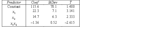
An economist is in the process of developing a model to predict the price of gold. She believes that the two most important variables are the price of a barrel of oil  and the interest rate
  She proposes the first-order model with interaction:
  .
.
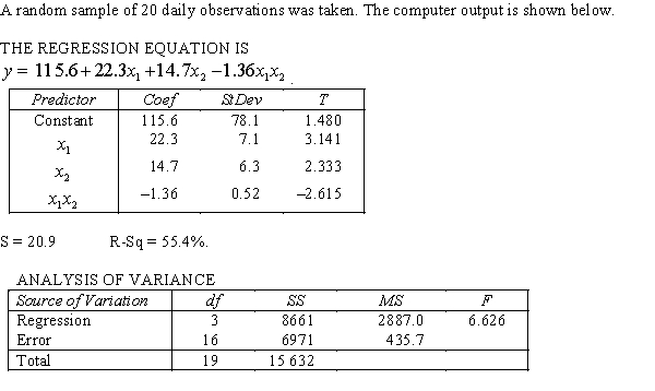
A random sample of 20 daily observations was taken. The computer output is shown below.
THE REGRESSION EQUATION IS Is there sufficient evidence at the 1% significance level to conclude that the price of a barrel of oil and the price of gold are linearly related?
and the interest rate She proposes the first-order model with interaction: .A random sample of 20 daily observations was taken. The computer output is shown below.
THE REGRESSION EQUATION IS
Is there sufficient evidence at the 1% significance level to conclude that the price of a barrel of oil and the price of gold are linearly related? سؤال
A traffic consultant has analysed the factors that affect the number of traffic fatalities. She has come to the conclusion that two important variables are the number of cars and the number of tractor-trailer trucks. She proposed the second-order model with interaction: 
 .
.
Where:
y = number of annual fatalities per shire. = number of cars registered in the shire (in units of 10 000).
  = number of trucks registered in the shire (in units of 1000).
The computer output (based on a random sample of 35 shires) is shown below.
THE REGRESSION EQUATION IS
 .
.  S = 15.2 R-Sq = 47.2%.
ANALYSIS OF VARIANCE Test at the 1% significance level to determine whether the
  term should be retained in the model.
.Where:
y = number of annual fatalities per shire.
= number of cars registered in the shire (in units of 10 000). = number of trucks registered in the shire (in units of 1000).The computer output (based on a random sample of 35 shires) is shown below.
THE REGRESSION EQUATION IS
. S = 15.2 R-Sq = 47.2%.ANALYSIS OF VARIANCE
Test at the 1% significance level to determine whether the term should be retained in the model. سؤال
A professor of accounting wanted to develop a multiple regression model to predict the students' grades in her fourth-year accounting course. She decides that the two most important factors are the student's grade point average (GPA) in the first three years and the student's major. She proposes the model:  .
.
where
y
= fourth-year accounting course mark (out of 100). = GPA in first three years (range 0 to 12).
  = 1 if student's major is accounting.
= 0 if not. = 1 if student's major is finance.
= 0 if not.
The computer output is shown below.
THE REGRESSION EQUATION IS
 .
.  S = 15.0 R-Sq = 44.2%.
  Do these results allow us to conclude at the 1% significance level that on average finance majors outperform those whose majors are not accounting or finance?
.where
y
= fourth-year accounting course mark (out of 100).
= GPA in first three years (range 0 to 12). = 1 if student's major is accounting.= 0 if not.
= 1 if student's major is finance.= 0 if not.
The computer output is shown below.
THE REGRESSION EQUATION IS
. S = 15.0 R-Sq = 44.2%. Do these results allow us to conclude at the 1% significance level that on average finance majors outperform those whose majors are not accounting or finance? سؤال
A traffic consultant has analysed the factors that affect the number of traffic fatalities. She has come to the conclusion that two important variables are the number of cars and the number of tractor-trailer trucks. She proposed the second-order model with interaction: 
 .
.
Where:
y = number of annual fatalities per shire. = number of cars registered in the shire (in units of 10 000).
  = number of trucks registered in the shire (in units of 1000).
The computer output (based on a random sample of 35 shires) is shown below.
THE REGRESSION EQUATION IS
 .
.  S = 15.2 R-Sq = 47.2%.
ANALYSIS OF VARIANCE Test at the 1% significance level to determine whether the interaction term should be retained in the model.
.Where:
y = number of annual fatalities per shire.
= number of cars registered in the shire (in units of 10 000). = number of trucks registered in the shire (in units of 1000).The computer output (based on a random sample of 35 shires) is shown below.
THE REGRESSION EQUATION IS
. S = 15.2 R-Sq = 47.2%.ANALYSIS OF VARIANCE
Test at the 1% significance level to determine whether the interaction term should be retained in the model. سؤال
A traffic consultant has analysed the factors that affect the number of traffic fatalities. She has come to the conclusion that two important variables are the number of cars and the number of tractor-trailer trucks. She proposed the second-order model with interaction: 
 .
.
Where:
y = number of annual fatalities per shire. = number of cars registered in the shire (in units of 10 000).
  = number of trucks registered in the shire (in units of 1000).
The computer output (based on a random sample of 35 shires) is shown below.
THE REGRESSION EQUATION IS
 .
.  S = 15.2 R-Sq = 47.2%.
ANALYSIS OF VARIANCE What is the multiple coefficient of determination? What does this statistic tell you about the model?
.Where:
y = number of annual fatalities per shire.
= number of cars registered in the shire (in units of 10 000). = number of trucks registered in the shire (in units of 1000).The computer output (based on a random sample of 35 shires) is shown below.
THE REGRESSION EQUATION IS
. S = 15.2 R-Sq = 47.2%.ANALYSIS OF VARIANCE
What is the multiple coefficient of determination? What does this statistic tell you about the model? سؤال
An economist is in the process of developing a model to predict the price of gold. She believes that the two most important variables are the price of a barrel of oil  and the interest rate
  She proposes the first-order model with interaction:
  .
.
A random sample of 20 daily observations was taken. The computer output is shown below.
THE REGRESSION EQUATION IS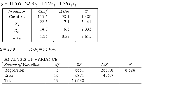 Is there sufficient evidence at the 1% significance level to conclude that the interest rate and the price of gold are linearly related?
and the interest rate She proposes the first-order model with interaction: .A random sample of 20 daily observations was taken. The computer output is shown below.
THE REGRESSION EQUATION IS
Is there sufficient evidence at the 1% significance level to conclude that the interest rate and the price of gold are linearly related? سؤال
A traffic consultant has analysed the factors that affect the number of traffic fatalities. She has come to the conclusion that two important variables are the number of cars and the number of tractor-trailer trucks. She proposed the second-order model with interaction: 
 .
.
Where:
y = number of annual fatalities per shire. = number of cars registered in the shire (in units of 10 000).
  = number of trucks registered in the shire (in units of 1000).
The computer output (based on a random sample of 35 shires) is shown below.
THE REGRESSION EQUATION IS
 .
.  S = 15.2 R-Sq = 47.2%.
ANALYSIS OF VARIANCE What does the coefficient of
  tell you about the model?
.Where:
y = number of annual fatalities per shire.
= number of cars registered in the shire (in units of 10 000). = number of trucks registered in the shire (in units of 1000).The computer output (based on a random sample of 35 shires) is shown below.
THE REGRESSION EQUATION IS
. S = 15.2 R-Sq = 47.2%.ANALYSIS OF VARIANCE
What does the coefficient of tell you about the model? سؤال
An economist is analysing the incomes of professionals (physicians, dentists and lawyers). He realises that an important factor is the number of years of experience. However, he wants to know if there are differences among the three professional groups. He takes a random sample of 125 professionals and estimates the multiple regression model:  .
.
where
y
= annual income (in $1000). = years of experience.
  = 1 if physician.
= 0 if not. = 1 if dentist.
= 0 if not.
The computer output is shown below.
THE REGRESSION EQUATION IS
 .
.  S = 42.6 R-Sq = 30.9%.
  Is there enough evidence at the1% significant level to conclude that physicians earn more on average than lawyers?
.where
y
= annual income (in $1000).
= years of experience. = 1 if physician.= 0 if not.
= 1 if dentist.= 0 if not.
The computer output is shown below.
THE REGRESSION EQUATION IS
. S = 42.6 R-Sq = 30.9%. Is there enough evidence at the1% significant level to conclude that physicians earn more on average than lawyers? سؤال
An economist is in the process of developing a model to predict the price of gold. She believes that the two most important variables are the price of a barrel of oil  and the interest rate
  She proposes the first-order model with interaction:
  .
.
A random sample of 20 daily observations was taken. The computer output is shown below.
THE REGRESSION EQUATION IS
 .
.  S = 20.9 R-Sq = 55.4%.
  Interpret the coefficient
  .
.
and the interest rate She proposes the first-order model with interaction: .A random sample of 20 daily observations was taken. The computer output is shown below.
THE REGRESSION EQUATION IS
. S = 20.9 R-Sq = 55.4%. Interpret the coefficient . سؤال
An economist is in the process of developing a model to predict the price of gold. She believes that the two most important variables are the price of a barrel of oil  and the interest rate
  She proposes the first-order model with interaction:
 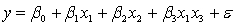 .
.
A random sample of 20 daily observations was taken. The computer output is shown below.
THE REGRESSION EQUATION IS
 .
.  S = 20.9 R-Sq = 55.4%.
 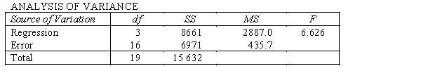 Do these results allow us at the 5% significance level to conclude that the model is useful in predicting the price of gold?
and the interest rate She proposes the first-order model with interaction: .A random sample of 20 daily observations was taken. The computer output is shown below.
THE REGRESSION EQUATION IS
. S = 20.9 R-Sq = 55.4%. Do these results allow us at the 5% significance level to conclude that the model is useful in predicting the price of gold? سؤال
An economist is in the process of developing a model to predict the price of gold. She believes that the two most important variables are the price of a barrel of oil  and the interest rate
  She proposes the first-order model with interaction:
  .
.  Is there sufficient evidence at the 1% significance level to conclude that the interaction term should be retained?
and the interest rate She proposes the first-order model with interaction: . Is there sufficient evidence at the 1% significance level to conclude that the interaction term should be retained? سؤال
An economist is analysing the incomes of professionals (physicians, dentists and lawyers). He realises that an important factor is the number of years of experience. However, he wants to know if there are differences among the three professional groups. He takes a random sample of 125 professionals and estimates the multiple regression model:  .
.
where
y
= annual income (in $1000). = years of experience.
  = 1 if physician.
= 0 if not. = 1 if dentist.
= 0 if not.
The computer output is shown below.
THE REGRESSION EQUATION IS
 .
.  S = 42.6 R-Sq = 30.9%.
 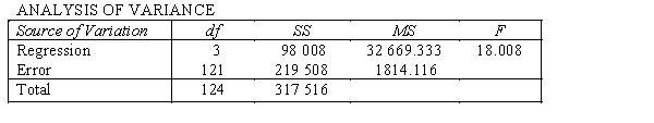 Do these results allow us to conclude at the 1% significance level that the model is useful in predicting the income of professionals?
.where
y
= annual income (in $1000).
= years of experience. = 1 if physician.= 0 if not.
= 1 if dentist.= 0 if not.
The computer output is shown below.
THE REGRESSION EQUATION IS
. S = 42.6 R-Sq = 30.9%. Do these results allow us to conclude at the 1% significance level that the model is useful in predicting the income of professionals? سؤال
A professor of accounting wanted to develop a multiple regression model to predict the students' grades in her fourth-year accounting course. She decides that the two most important factors are the student's grade point average (GPA) in the first three years and the student's major. She proposes the model:  .
.
where
y
= fourth-year accounting course mark (out of 100). = GPA in first three years (range 0 to 12).
  = 1 if student's major is accounting.
= 0 if not. = 1 if student's major is finance.
= 0 if not.
The computer output is shown below.
THE REGRESSION EQUATION IS
 .
.  S = 15.0 R-Sq = 44.2%.
  Do these results allow us to conclude at the 1% significance level that on average accounting majors outperform those whose majors are not accounting or finance?
.where
y
= fourth-year accounting course mark (out of 100).
= GPA in first three years (range 0 to 12). = 1 if student's major is accounting.= 0 if not.
= 1 if student's major is finance.= 0 if not.
The computer output is shown below.
THE REGRESSION EQUATION IS
. S = 15.0 R-Sq = 44.2%. Do these results allow us to conclude at the 1% significance level that on average accounting majors outperform those whose majors are not accounting or finance? سؤال
An economist is analysing the incomes of professionals (physicians, dentists and lawyers). He realises that an important factor is the number of years of experience. However, he wants to know if there are differences among the three professional groups. He takes a random sample of 125 professionals and estimates the multiple regression model:  .
.
where
y
= annual income (in $1000). = years of experience.
  = 1 if physician.
= 0 if not. = 1 if dentist.
= 0 if not.
The computer output is shown below.
THE REGRESSION EQUATION IS
 .
.  S = 42.6 R-Sq = 30.9%.
  Is there enough evidence at the 10% significance level to conclude that dentists earn less on average than lawyers?
.where
y
= annual income (in $1000).
= years of experience. = 1 if physician.= 0 if not.
= 1 if dentist.= 0 if not.
The computer output is shown below.
THE REGRESSION EQUATION IS
. S = 42.6 R-Sq = 30.9%. Is there enough evidence at the 10% significance level to conclude that dentists earn less on average than lawyers? سؤال
A traffic consultant has analysed the factors that affect the number of traffic fatalities. She has come to the conclusion that two important variables are the number of cars and the number of tractor-trailer trucks. She proposed the second-order model with interaction: 
 .
.
Where:
y = number of annual fatalities per shire. = number of cars registered in the shire (in units of 10 000).
  = number of trucks registered in the shire (in units of 1000).
The computer output (based on a random sample of 35 shires) is shown below.
THE REGRESSION EQUATION IS
 .
.  S = 15.2 R-Sq = 47.2%.
ANALYSIS OF VARIANCE What does the coefficient of
  tell you about the model?
.Where:
y = number of annual fatalities per shire.
= number of cars registered in the shire (in units of 10 000). = number of trucks registered in the shire (in units of 1000).The computer output (based on a random sample of 35 shires) is shown below.
THE REGRESSION EQUATION IS
. S = 15.2 R-Sq = 47.2%.ANALYSIS OF VARIANCE
What does the coefficient of tell you about the model? سؤال
A professor of accounting wanted to develop a multiple regression model to predict the students' grades in her fourth-year accounting course. She decides that the two most important factors are the student's grade point average (GPA) in the first three years and the student's major. She proposes the model: 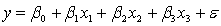 .
.
where
y
= fourth-year accounting course mark (out of 100). = GPA in first three years (range 0 to 12).
  = 1 if student's major is accounting.
= 0 if not. = 1 if student's major is finance.
= 0 if not.
The computer output is shown below.
THE REGRESSION EQUATION IS
 .
.  S = 15.0 R-Sq = 44.2%.
 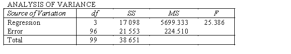 Do these results allow us to conclude at the 1% significance level that the model is useful in predicting the fourth-year accounting course mark?
.where
y
= fourth-year accounting course mark (out of 100).
= GPA in first three years (range 0 to 12). = 1 if student's major is accounting.= 0 if not.
= 1 if student's major is finance.= 0 if not.
The computer output is shown below.
THE REGRESSION EQUATION IS
. S = 15.0 R-Sq = 44.2%. Do these results allow us to conclude at the 1% significance level that the model is useful in predicting the fourth-year accounting course mark?
فتح الحزمة
قم بالتسجيل لفتح البطاقات في هذه المجموعة!
Unlock Deck
Unlock Deck
1/92
العب
ملء الشاشة (f)
Deck 20: Model Building
1
In explaining the income earned by university graduates, which of the following independent variables is best represented by an indicator variable in a regression model?
A) Grade point average.
B) Gender
C) Number of years since graduating from high school.
D) Age
A) Grade point average.
B) Gender
C) Number of years since graduating from high school.
D) Age
B
2
The model + is referred to as a:
A) first-order model with two predictor variables with no interaction.
B) first-order model with two predictor variables with interaction.
C) second-order model with three predictor variables with no interaction.
D) second-order model with three predictor variables with interaction.
+ is referred to as a:A) first-order model with two predictor variables with no interaction.
B) first-order model with two predictor variables with interaction.
C) second-order model with three predictor variables with no interaction.
D) second-order model with three predictor variables with interaction.
B
3
Which of the following best describes Stepwise regression?
A) Stepwise regression may involve adding one independent variable at a time.
B) Stepwise regression may involve deleting one independent variable at a time.
C) Stepwise regression may involve dividing one independent variable at a time.
D) Stepwise regression may involve adding or deleting one independent variable at a time.
D
4
In explaining starting salaries for graduates of computer science programs, which of the following independent variables would not be adequately represented with a dummy variable?
A) Grade point average.
B) Gender.
C) Race.
D) Marital status.
A) Grade point average.
B) Gender.
C) Race.
D) Marital status.
فتح الحزمة
افتح القفل للوصول البطاقات البالغ عددها 92 في هذه المجموعة.
فتح الحزمة
k this deck
5
Which of the following describes the numbers that an indicator variable can have in a regression model?
A) 0 and 1
B) 1 and 2
C) 0, 1 and 2
D) None of these choices are correct.
A) 0 and 1
B) 1 and 2
C) 0, 1 and 2
D) None of these choices are correct.
فتح الحزمة
افتح القفل للوصول البطاقات البالغ عددها 92 في هذه المجموعة.
فتح الحزمة
k this deck
6
The model + is referred to as a:
A) first-order model with one predictor variable.
B) first-order model with two predictor variables.
C) second-order model with one predictor variable.
D) second-order model with two predictor variables.
+ is referred to as a:A) first-order model with one predictor variable.
B) first-order model with two predictor variables.
C) second-order model with one predictor variable.
D) second-order model with two predictor variables.
فتح الحزمة
افتح القفل للوصول البطاقات البالغ عددها 92 في هذه المجموعة.
فتح الحزمة
k this deck
7
Which of the following is another name for a dummy variable?
A) Independent variable
B) Dependent variable
C) Indicator variable
D) Y variable
A) Independent variable
B) Dependent variable
C) Indicator variable
D) Y variable
فتح الحزمة
افتح القفل للوصول البطاقات البالغ عددها 92 في هذه المجموعة.
فتح الحزمة
k this deck
8
The graph of the model is shaped like a straight line going upwards.
is shaped like a straight line going upwards. فتح الحزمة
افتح القفل للوصول البطاقات البالغ عددها 92 في هذه المجموعة.
فتح الحزمة
k this deck
9
Suppose that the estimated regression equation for 200 business graduates is ŷ = 20 000 + 2000x + 1500I,
Where y is the starting salary, x is the grade point average and I is an indicator variable that takes the value of 1 if the student is a computer information systems major and 0 if not. A business administration major graduate with a grade point average of 4 would have an average starting salary of:
A) $20 000.
B) $26 000.
C) $29 500.
D) $28 000.
فتح الحزمة
افتح القفل للوصول البطاقات البالغ عددها 92 في هذه المجموعة.
فتح الحزمة
k this deck
10
In general, to represent a categorical independent variable that has m possible categories, which of the following is the number of dummy variables that can be used in the regression model?
A) (m + 1) dummy variables.
B) m dummy variables.
C) (1 − m) dummy variables.
D) (m - 1) dummy variables.
A) (m + 1) dummy variables.
B) m dummy variables.
C) (1 − m) dummy variables.
D) (m - 1) dummy variables.
فتح الحزمة
افتح القفل للوصول البطاقات البالغ عددها 92 في هذه المجموعة.
فتح الحزمة
k this deck
11
In a stepwise regression procedure, if two independent variables are highly correlated, then:
A) both variables will enter the equation.
B) only one variable will enter the equation.
C) neither variable will enter the equation.
D) None of these choices are correct.
A) both variables will enter the equation.
B) only one variable will enter the equation.
C) neither variable will enter the equation.
D) None of these choices are correct.
فتح الحزمة
افتح القفل للوصول البطاقات البالغ عددها 92 في هذه المجموعة.
فتح الحزمة
k this deck
12
Suppose that the sample regression equation of a model is . If we examine the relationship between and y for four different values of , we observe that the four equations produced differ only in the intercept term.
. If we examine the relationship between and y for four different values of , we observe that the four equations produced differ only in the intercept term. فتح الحزمة
افتح القفل للوصول البطاقات البالغ عددها 92 في هذه المجموعة.
فتح الحزمة
k this deck
13
When we plot x versus y, the graph of the model + is shaped like a:
A) straight line going upwards.
B) straight line going downwards.
C) circle.
D) parabola.
+ is shaped like a:A) straight line going upwards.
B) straight line going downwards.
C) circle.
D) parabola.
فتح الحزمة
افتح القفل للوصول البطاقات البالغ عددها 92 في هذه المجموعة.
فتح الحزمة
k this deck
14
In explaining the amount of money spent on children's clothes each month, which of the following independent variables is best represented with an indicator variable?
A) Age.
B) Height.
C) Gender.
D) Weight.
A) Age.
B) Height.
C) Gender.
D) Weight.
فتح الحزمة
افتح القفل للوصول البطاقات البالغ عددها 92 في هذه المجموعة.
فتح الحزمة
k this deck
15
Suppose that the sample regression line of a first order model is . If we examine the relationship between y and for four different values of , we observe that the:
A) effect of x on y remains the same no matter what the value of x .
B) effect of x on y remains the same no matter what the value of x .
C) only difference in the four equations produced is the coefficient of x .
D) None of these choices are correct.
. If we examine the relationship between y and for four different values of , we observe that the:A) effect of x on y remains the same no matter what the value of x .
B) effect of x on y remains the same no matter what the value of x .
C) only difference in the four equations produced is the coefficient of x .
D) None of these choices are correct.
فتح الحزمة
افتح القفل للوصول البطاقات البالغ عددها 92 في هذه المجموعة.
فتح الحزمة
k this deck
16
In explaining students' test scores, which of the following independent variables would not be adequately represented by an indicator variable?
A) Gender
B) Cultural background
C) Number of hours studying for the test
D) Marital status
A) Gender
B) Cultural background
C) Number of hours studying for the test
D) Marital status
فتح الحزمة
افتح القفل للوصول البطاقات البالغ عددها 92 في هذه المجموعة.
فتح الحزمة
k this deck
17
For the regression equation , which combination of and , respectively, results in the largest average value of y?
A) 3 and 5.
B) 5 and 3.
C) 6 and 3.
D) 3 and 6.
, which combination of and , respectively, results in the largest average value of y?A) 3 and 5.
B) 5 and 3.
C) 6 and 3.
D) 3 and 6.
فتح الحزمة
افتح القفل للوصول البطاقات البالغ عددها 92 في هذه المجموعة.
فتح الحزمة
k this deck
18
Which of the following is not an advantage of multiple regression as compared with analysis of variance?
A) Multiple regression can be used to estimate the relationship between the dependent variable and independent variables.
B) Multiple regression handles qualitative variables better than analysis of variance.
C) Multiple regression handles problems with more than two independent variables better than analysis of variance.
D) All of the above are advantages of multiple regression as compared with analysis of variance.
فتح الحزمة
افتح القفل للوصول البطاقات البالغ عددها 92 في هذه المجموعة.
فتح الحزمة
k this deck
19
Suppose that the sample regression equation of a model is . If we examine the relationship between and y for three different values of , we observe that the:
A) three equations produced differ only in the intercept.
B) coefficient of remains unchanged.
C) coefficient of varies.
D) three equations produced differ not only in the intercept term but the coefficient of , also varies.
. If we examine the relationship between and y for three different values of , we observe that the:A) three equations produced differ only in the intercept.
B) coefficient of remains unchanged.
C) coefficient of varies.
D) three equations produced differ not only in the intercept term but the coefficient of , also varies.
فتح الحزمة
افتح القفل للوصول البطاقات البالغ عددها 92 في هذه المجموعة.
فتح الحزمة
k this deck
20
The following model + is used whenever the statistician believes that, on average, y is linearly related to:
A) , and the predictor variables do not interact.
B) , and the predictor variables do not interact.
C) and the predictor variables do not interact or to , and the predictor variables do not interact.
D) and the predictor variables do not interact and to , and the predictor variables do not interact.
+ is used whenever the statistician believes that, on average, y is linearly related to:A)
, and the predictor variables do not interact.B)
, and the predictor variables do not interact.C)
and the predictor variables do not interact or to , and the predictor variables do not interact.D)
and the predictor variables do not interact and to , and the predictor variables do not interact. فتح الحزمة
افتح القفل للوصول البطاقات البالغ عددها 92 في هذه المجموعة.
فتح الحزمة
k this deck
21
Stepwise regression is an iterative procedure that can only add one independent variable at a time.
فتح الحزمة
افتح القفل للوصول البطاقات البالغ عددها 92 في هذه المجموعة.
فتح الحزمة
k this deck
22
The model
is referred to as a first-order model with two predictor variables with no interaction.
is referred to as a first-order model with two predictor variables with no interaction.
فتح الحزمة
افتح القفل للوصول البطاقات البالغ عددها 92 في هذه المجموعة.
فتح الحزمة
k this deck
23
In the first-order model ŷ = 8 + 3x1 +5x2, a unit increase in , while holding constant, increases the value of on average by 3 units.
, while holding constant, increases the value of on average by 3 units. فتح الحزمة
افتح القفل للوصول البطاقات البالغ عددها 92 في هذه المجموعة.
فتح الحزمة
k this deck
24
In the first-order model = 60 + 40x1 -10x2 + 5x1x2, a unit increase in x1, while holding x2 constant at 1, increases the value of on average by 45 units.
= 60 + 40x1 -10x2 + 5x1x2, a unit increase in x1, while holding x2 constant at 1, increases the value of on average by 45 units. فتح الحزمة
افتح القفل للوصول البطاقات البالغ عددها 92 في هذه المجموعة.
فتح الحزمة
k this deck
25
In a first-order model with two predictors, and , an interaction term may be used when the relationship between the dependent variable and the predictor variables is linear.
and , an interaction term may be used when the relationship between the dependent variable and the predictor variables is linear. فتح الحزمة
افتح القفل للوصول البطاقات البالغ عددها 92 في هذه المجموعة.
فتح الحزمة
k this deck
26
Regression analysis allows the statistics practitioner to use mathematical models to realistically describe relationships between the dependent variable and independent variables.
فتح الحزمة
افتح القفل للوصول البطاقات البالغ عددها 92 في هذه المجموعة.
فتح الحزمة
k this deck
27
Suppose that the sample regression line of a first-order model is . If we examine the relationship between y and for three different values of , we observe that the effect of on remains the same no matter what the value of .
. If we examine the relationship between y and for three different values of , we observe that the effect of on remains the same no matter what the value of . فتح الحزمة
افتح القفل للوصول البطاقات البالغ عددها 92 في هذه المجموعة.
فتح الحزمة
k this deck
28
In general, to represent a nominal independent variable that has n possible categories, we would create n dummy variables.
فتح الحزمة
افتح القفل للوصول البطاقات البالغ عددها 92 في هذه المجموعة.
فتح الحزمة
k this deck
29
In explaining the amount of money spent on children's toys during Christmas each year, the independent variable 'gender' is best represented by a dummy variable.
فتح الحزمة
افتح القفل للوصول البطاقات البالغ عددها 92 في هذه المجموعة.
فتح الحزمة
k this deck
30
In a stepwise regression procedure, if two independent variables are highly correlated, then one variable usually eliminates the second variable.
فتح الحزمة
افتح القفل للوصول البطاقات البالغ عددها 92 في هذه المجموعة.
فتح الحزمة
k this deck
31
Stepwise regression is especially useful when there are many independent variables.
فتح الحزمة
افتح القفل للوصول البطاقات البالغ عددها 92 في هذه المجموعة.
فتح الحزمة
k this deck
32
In the first-order model
, a unit increase in , while holding constant at a value of 3, decreases the value of on average by 3 units.
, a unit increase in , while holding constant at a value of 3, decreases the value of on average by 3 units.
فتح الحزمة
افتح القفل للوصول البطاقات البالغ عددها 92 في هذه المجموعة.
فتح الحزمة
k this deck
33
In the first-order regression model ŷ = 12 + 6x1 +8x2 + 4x1x2, a unit increase in x1 increases the value of on average by 6 units.
on average by 6 units. فتح الحزمة
افتح القفل للوصول البطاقات البالغ عددها 92 في هذه المجموعة.
فتح الحزمة
k this deck
34
In the first-order model
, a unit increase in , while holding constant at a value of 2, decreases the value of on average by 8 units.
, a unit increase in , while holding constant at a value of 2, decreases the value of on average by 8 units.
فتح الحزمة
افتح القفل للوصول البطاقات البالغ عددها 92 في هذه المجموعة.
فتح الحزمة
k this deck
35
Suppose that the sample regression equation of a model is
. If we examine the relationship between y and for = 1, 2 and 3, we observe that the three equations produced not only differ in the intercept term, but the coefficient of also varies.
. If we examine the relationship between y and for = 1, 2 and 3, we observe that the three equations produced not only differ in the intercept term, but the coefficient of also varies.
فتح الحزمة
افتح القفل للوصول البطاقات البالغ عددها 92 في هذه المجموعة.
فتح الحزمة
k this deck
36
In regression analysis, indicator variables may be used as independent variables.
فتح الحزمة
افتح القفل للوصول البطاقات البالغ عددها 92 في هذه المجموعة.
فتح الحزمة
k this deck
37
The model is used whenever the statistician believes that, on average, is linearly related to and , and the predictor variables do not interact.
is used whenever the statistician believes that, on average, is linearly related to and , and the predictor variables do not interact. فتح الحزمة
افتح القفل للوصول البطاقات البالغ عددها 92 في هذه المجموعة.
فتح الحزمة
k this deck
38
The model y = 0 + 1x + is referred to as a simple linear regression model.
is referred to as a simple linear regression model. فتح الحزمة
افتح القفل للوصول البطاقات البالغ عددها 92 في هذه المجموعة.
فتح الحزمة
k this deck
39
The model y = 0 + 1x + 2x2 + … + pxp + is referred to as a polynomial model with p predictor variables.
is referred to as a polynomial model with p predictor variables. فتح الحزمة
افتح القفل للوصول البطاقات البالغ عددها 92 في هذه المجموعة.
فتح الحزمة
k this deck
40
The model is referred to as a second-order model with two predictor variables with interaction.
is referred to as a second-order model with two predictor variables with interaction. فتح الحزمة
افتح القفل للوصول البطاقات البالغ عددها 92 في هذه المجموعة.
فتح الحزمة
k this deck
41
Consider the following data for two variables, x and y. Use Excel to develop an estimated regression equation of the form ? = b0 +b1x + b2x2..
فتح الحزمة
افتح القفل للوصول البطاقات البالغ عددها 92 في هذه المجموعة.
فتح الحزمة
k this deck
42
Consider the following data for two variables, x and y, where x is the age of a particular make of car
and y is the selling price, in thousands of dollars. Use Excel to test whether the population slope is positive, at the 1% level of significance.
and y is the selling price, in thousands of dollars.
Use Excel to test whether the population slope is positive, at the 1% level of significance. فتح الحزمة
افتح القفل للوصول البطاقات البالغ عددها 92 في هذه المجموعة.
فتح الحزمة
k this deck
43
Consider the following data for two variables, x and y. Use the model in = 66.799 -7.307x + 0.324x2 to predict the value of y when x = 10.
= 66.799 -7.307x + 0.324x2 to predict the value of y when x = 10. فتح الحزمة
افتح القفل للوصول البطاقات البالغ عددها 92 في هذه المجموعة.
فتح الحزمة
k this deck
44
A regression analysis was performed to study the relationship between a dependent variable and four independent variables. The following information was obtained:
r2 = 0.95, SSR = 9800, n = 50.
ANOVA Test the overall validity of the model at the 5% significance level.
r2 = 0.95, SSR = 9800, n = 50.
ANOVA
Test the overall validity of the model at the 5% significance level. فتح الحزمة
افتح القفل للوصول البطاقات البالغ عددها 92 في هذه المجموعة.
فتح الحزمة
k this deck
45
Consider the following data for two variables, x and y. Use Excel to determine whether there is sufficient evidence at the 1% significance level to infer that the relationship between y, x and in = 66.799 -7.307x + 0.324x2 is significant.
= 66.799 -7.307x + 0.324x2 is significant. فتح الحزمة
افتح القفل للوصول البطاقات البالغ عددها 92 في هذه المجموعة.
فتح الحزمة
k this deck
46
In regression analysis, we can use 11 indicator variables to represent 12 months of the year.
فتح الحزمة
افتح القفل للوصول البطاقات البالغ عددها 92 في هذه المجموعة.
فتح الحزمة
k this deck
47
A regression analysis was performed to study the relationship between a dependent variable and four independent variables. The following information was obtained:
r2 = 0.95, SSR = 9800, n = 50.
Create the ANOVA table.
r2 = 0.95, SSR = 9800, n = 50.
Create the ANOVA table.
فتح الحزمة
افتح القفل للوصول البطاقات البالغ عددها 92 في هذه المجموعة.
فتح الحزمة
k this deck
48
Consider the following data for two variables, x and y. Use Excel to find the coefficient of determination. What does this statistic tell you about this curvilinear model?
Use Excel to find the coefficient of determination. What does this statistic tell you about this curvilinear model? فتح الحزمة
افتح القفل للوصول البطاقات البالغ عددها 92 في هذه المجموعة.
فتح الحزمة
k this deck
49
An avid football fan was in the process of examining the factors that determine the success or failure of football teams. He noticed that teams with many rookies and teams with many veterans seem to do quite poorly. To further analyse his beliefs, he took a random sample of 20 teams and proposed a second-order model with one independent variable. The selected model is: .
where
y = winning team's percentage.
x = average years of professional experience.
The computer output is shown below:
THE REGRESSION EQUATION IS: S = 16.1 R-Sq = 43.9%.
ANALYSIS OF VARIANCE Test to determine at the 10% significance level if the linear term should be retained.
.where
y = winning team's percentage.
x = average years of professional experience.
The computer output is shown below:
THE REGRESSION EQUATION IS:
S = 16.1 R-Sq = 43.9%.ANALYSIS OF VARIANCE
Test to determine at the 10% significance level if the linear term should be retained. فتح الحزمة
افتح القفل للوصول البطاقات البالغ عددها 92 في هذه المجموعة.
فتح الحزمة
k this deck
50
A traffic consultant has analysed the factors that affect the number of traffic fatalities. She has come to the conclusion that two important variables are the number of cars and the number of tractor-trailer trucks. She proposed the second-order model with interaction: .
Where:
y = number of annual fatalities per shire. = number of cars registered in the shire (in units of 10 000). = number of trucks registered in the shire (in units of 1000).
The computer output (based on a random sample of 35 shires) is shown below.
THE REGRESSION EQUATION IS . S = 15.2 R-Sq = 47.2%.
ANALYSIS OF VARIANCE Is there enough evidence at the 5% significance level to conclude that the model is useful in predicting the number of fatalities?
.Where:
y = number of annual fatalities per shire.
= number of cars registered in the shire (in units of 10 000). = number of trucks registered in the shire (in units of 1000).The computer output (based on a random sample of 35 shires) is shown below.
THE REGRESSION EQUATION IS
. S = 15.2 R-Sq = 47.2%.ANALYSIS OF VARIANCE
Is there enough evidence at the 5% significance level to conclude that the model is useful in predicting the number of fatalities? فتح الحزمة
افتح القفل للوصول البطاقات البالغ عددها 92 في هذه المجموعة.
فتح الحزمة
k this deck
51
A regression analysis involving 40 observations and five independent variables revealed that the total variation in the dependent variable y is 1080 and that the mean square for error is 30.
Create the ANOVA table.
Create the ANOVA table.
فتح الحزمة
افتح القفل للوصول البطاقات البالغ عددها 92 في هذه المجموعة.
فتح الحزمة
k this deck
52
Consider the following data for two variables, x and y. Use Excel to find the coefficient of determination. What does this statistic tell you about this simple linear model?
Use Excel to find the coefficient of determination. What does this statistic tell you about this simple linear model? فتح الحزمة
افتح القفل للوصول البطاقات البالغ عددها 92 في هذه المجموعة.
فتح الحزمة
k this deck
53
An indicator variable (also called a dummy variable) is a variable that can assume either one of two values (usually 0 and 1), where one value represents the existence of a certain condition, and the other value indicates that the condition does not hold.
فتح الحزمة
افتح القفل للوصول البطاقات البالغ عددها 92 في هذه المجموعة.
فتح الحزمة
k this deck
54
Consider the following data for two variables, x and y. Use Excel to develop a scatter diagram for the data. Does the scatter diagram suggest an estimated regression equation of the form ŷ = b0 +b1x + b2x2? Explain.
Use Excel to develop a scatter diagram for the data. Does the scatter diagram suggest an estimated regression equation of the form ŷ = b0 +b1x + b2x2? Explain. فتح الحزمة
افتح القفل للوصول البطاقات البالغ عددها 92 في هذه المجموعة.
فتح الحزمة
k this deck
55
An avid football fan was in the process of examining the factors that determine the success or failure of football teams. He noticed that teams with many rookies and teams with many veterans seem to do quite poorly. To further analyse his beliefs, he took a random sample of 20 teams and proposed a second-order model with one independent variable. The selected model is: .
where
y = winning team's percentage.
x = average years of professional experience.
The computer output is shown below:
THE REGRESSION EQUATION IS: S = 16.1 R-Sq = 43.9%.
ANALYSIS OF VARIANCE What is the coefficient of determination? Explain what this statistic tells you about the model.
.where
y = winning team's percentage.
x = average years of professional experience.
The computer output is shown below:
THE REGRESSION EQUATION IS:
S = 16.1 R-Sq = 43.9%.ANALYSIS OF VARIANCE
What is the coefficient of determination? Explain what this statistic tells you about the model. فتح الحزمة
افتح القفل للوصول البطاقات البالغ عددها 92 في هذه المجموعة.
فتح الحزمة
k this deck
56
We interpret the coefficients in a multiple regression model by holding all variables in the model constant.
فتح الحزمة
افتح القفل للوصول البطاقات البالغ عددها 92 في هذه المجموعة.
فتح الحزمة
k this deck
57
An avid football fan was in the process of examining the factors that determine the success or failure of football teams. He noticed that teams with many rookies and teams with many veterans seem to do quite poorly. To further analyse his beliefs, he took a random sample of 20 teams and proposed a second-order model with one independent variable. The selected model is: .
where
y = winning team's percentage.
x = average years of professional experience.
The computer output is shown below:
THE REGRESSION EQUATION IS: S = 16.1 R-Sq = 43.9%.
ANALYSIS OF VARIANCE Do these results allow us to conclude at the 5% significance level that the model is useful in predicting the team's winning percentage?
فتح الحزمة
افتح القفل للوصول البطاقات البالغ عددها 92 في هذه المجموعة.
فتح الحزمة
k this deck
58
A regression analysis involving 40 observations and five independent variables revealed that the total variation in the dependent variable y is 1080 and that the mean square for error is 30. Test the significance of the overall equation at the 5% level of significance.
Test the significance of the overall equation at the 5% level of significance. فتح الحزمة
افتح القفل للوصول البطاقات البالغ عددها 92 في هذه المجموعة.
فتح الحزمة
k this deck
59
An avid football fan was in the process of examining the factors that determine the success or failure of football teams. He noticed that teams with many rookies and teams with many veterans seem to do quite poorly. To further analyse his beliefs, he took a random sample of 20 teams and proposed a second-order model with one independent variable. The selected model is: .
where
y = winning team's percentage.
x = average years of professional experience.
The computer output is shown below:
THE REGRESSION EQUATION IS: S = 16.1 R-Sq = 43.9%.
ANALYSIS OF VARIANCE Test to determine at the 10% significance level whether the term should be retained.
.where
y = winning team's percentage.
x = average years of professional experience.
The computer output is shown below:
THE REGRESSION EQUATION IS:
S = 16.1 R-Sq = 43.9%.ANALYSIS OF VARIANCE
Test to determine at the 10% significance level whether the term should be retained. فتح الحزمة
افتح القفل للوصول البطاقات البالغ عددها 92 في هذه المجموعة.
فتح الحزمة
k this deck
60
Consider the following data for two variables, x and y, where x is the age of a particular make of car
and y is the selling price, in thousands of dollars. a. Use Excel to develop an estimated regression equation of the form = b0 +b1x.
b. Interpret the intercept.
c. Interpret the slope.
and y is the selling price, in thousands of dollars. a. Use Excel to develop an estimated regression equation of the form
= b0 +b1x.b. Interpret the intercept.
c. Interpret the slope.
فتح الحزمة
افتح القفل للوصول البطاقات البالغ عددها 92 في هذه المجموعة.
فتح الحزمة
k this deck
61
A traffic consultant has analysed the factors that affect the number of traffic fatalities. She has come to the conclusion that two important variables are the number of cars and the number of tractor-trailer trucks. She proposed the second-order model with interaction: .
Where:
y = number of annual fatalities per shire. = number of cars registered in the shire (in units of 10 000). = number of trucks registered in the shire (in units of 1000).
The computer output (based on a random sample of 35 shires) is shown below.
THE REGRESSION EQUATION IS . S = 15.2 R-Sq = 47.2%.
ANALYSIS OF VARIANCE Test at the 1% significance level to determine whether the term should be retained in the model.
.Where:
y = number of annual fatalities per shire.
= number of cars registered in the shire (in units of 10 000). = number of trucks registered in the shire (in units of 1000).The computer output (based on a random sample of 35 shires) is shown below.
THE REGRESSION EQUATION IS
. S = 15.2 R-Sq = 47.2%.ANALYSIS OF VARIANCE
Test at the 1% significance level to determine whether the term should be retained in the model. فتح الحزمة
افتح القفل للوصول البطاقات البالغ عددها 92 في هذه المجموعة.
فتح الحزمة
k this deck
62
An economist is analysing the incomes of professionals (physicians, dentists and lawyers). He realises that an important factor is the number of years of experience. However, he wants to know if there are differences among the three professional groups. He takes a random sample of 125 professionals and estimates the multiple regression model: .
where
y
= annual income (in $1000). = years of experience. = 1 if physician.
= 0 if not. = 1 if dentist.
= 0 if not.
The computer output is shown below.
THE REGRESSION EQUATION IS . S = 42.6 R-Sq = 30.9%. Is there enough evidence at the 5% significance level to conclude that income and experience are linearly related?
.where
y
= annual income (in $1000).
= years of experience. = 1 if physician.= 0 if not.
= 1 if dentist.= 0 if not.
The computer output is shown below.
THE REGRESSION EQUATION IS
. S = 42.6 R-Sq = 30.9%. Is there enough evidence at the 5% significance level to conclude that income and experience are linearly related? فتح الحزمة
افتح القفل للوصول البطاقات البالغ عددها 92 في هذه المجموعة.
فتح الحزمة
k this deck
63
A traffic consultant has analysed the factors that affect the number of traffic fatalities. She has come to the conclusion that two important variables are the number of cars and the number of tractor-trailer trucks. She proposed the second-order model with interaction: .
Where:
y = number of annual fatalities per shire. = number of cars registered in the shire (in units of 10 000). = number of trucks registered in the shire (in units of 1000).
The computer output (based on a random sample of 35 shires) is shown below.
THE REGRESSION EQUATION IS . S = 15.2 R-Sq = 47.2%.
ANALYSIS OF VARIANCE Test at the 1% significance level to determine whether the term should be retained in the model.
.Where:
y = number of annual fatalities per shire.
= number of cars registered in the shire (in units of 10 000). = number of trucks registered in the shire (in units of 1000).The computer output (based on a random sample of 35 shires) is shown below.
THE REGRESSION EQUATION IS
. S = 15.2 R-Sq = 47.2%.ANALYSIS OF VARIANCE
Test at the 1% significance level to determine whether the term should be retained in the model. فتح الحزمة
افتح القفل للوصول البطاقات البالغ عددها 92 في هذه المجموعة.
فتح الحزمة
k this deck
64
A traffic consultant has analysed the factors that affect the number of traffic fatalities. She has come to the conclusion that two important variables are the number of cars and the number of tractor-trailer trucks. She proposed the second-order model with interaction: .
Where:
y = number of annual fatalities per shire. = number of cars registered in the shire (in units of 10 000). = number of trucks registered in the shire (in units of 1000).
The computer output (based on a random sample of 35 shires) is shown below.
THE REGRESSION EQUATION IS . S = 15.2 R-Sq = 47.2%.
ANALYSIS OF VARIANCE Test at the 1% significance level to determine whether the term should be retained in the model.
.Where:
y = number of annual fatalities per shire.
= number of cars registered in the shire (in units of 10 000). = number of trucks registered in the shire (in units of 1000).The computer output (based on a random sample of 35 shires) is shown below.
THE REGRESSION EQUATION IS
. S = 15.2 R-Sq = 47.2%.ANALYSIS OF VARIANCE
Test at the 1% significance level to determine whether the term should be retained in the model. فتح الحزمة
افتح القفل للوصول البطاقات البالغ عددها 92 في هذه المجموعة.
فتح الحزمة
k this deck
65
An economist is in the process of developing a model to predict the price of gold. She believes that the two most important variables are the price of a barrel of oil and the interest rate She proposes the first-order model with interaction: .
A random sample of 20 daily observations was taken. The computer output is shown below.
THE REGRESSION EQUATION IS Is there sufficient evidence at the 1% significance level to conclude that the price of a barrel of oil and the price of gold are linearly related?
and the interest rate She proposes the first-order model with interaction: .A random sample of 20 daily observations was taken. The computer output is shown below.
THE REGRESSION EQUATION IS
Is there sufficient evidence at the 1% significance level to conclude that the price of a barrel of oil and the price of gold are linearly related? فتح الحزمة
افتح القفل للوصول البطاقات البالغ عددها 92 في هذه المجموعة.
فتح الحزمة
k this deck
66
A traffic consultant has analysed the factors that affect the number of traffic fatalities. She has come to the conclusion that two important variables are the number of cars and the number of tractor-trailer trucks. She proposed the second-order model with interaction: .
Where:
y = number of annual fatalities per shire. = number of cars registered in the shire (in units of 10 000). = number of trucks registered in the shire (in units of 1000).
The computer output (based on a random sample of 35 shires) is shown below.
THE REGRESSION EQUATION IS . S = 15.2 R-Sq = 47.2%.
ANALYSIS OF VARIANCE Test at the 1% significance level to determine whether the term should be retained in the model.
.Where:
y = number of annual fatalities per shire.
= number of cars registered in the shire (in units of 10 000). = number of trucks registered in the shire (in units of 1000).The computer output (based on a random sample of 35 shires) is shown below.
THE REGRESSION EQUATION IS
. S = 15.2 R-Sq = 47.2%.ANALYSIS OF VARIANCE
Test at the 1% significance level to determine whether the term should be retained in the model. فتح الحزمة
افتح القفل للوصول البطاقات البالغ عددها 92 في هذه المجموعة.
فتح الحزمة
k this deck
67
A professor of accounting wanted to develop a multiple regression model to predict the students' grades in her fourth-year accounting course. She decides that the two most important factors are the student's grade point average (GPA) in the first three years and the student's major. She proposes the model: .
where
y
= fourth-year accounting course mark (out of 100). = GPA in first three years (range 0 to 12). = 1 if student's major is accounting.
= 0 if not. = 1 if student's major is finance.
= 0 if not.
The computer output is shown below.
THE REGRESSION EQUATION IS . S = 15.0 R-Sq = 44.2%. Do these results allow us to conclude at the 1% significance level that on average finance majors outperform those whose majors are not accounting or finance?
.where
y
= fourth-year accounting course mark (out of 100).
= GPA in first three years (range 0 to 12). = 1 if student's major is accounting.= 0 if not.
= 1 if student's major is finance.= 0 if not.
The computer output is shown below.
THE REGRESSION EQUATION IS
. S = 15.0 R-Sq = 44.2%. Do these results allow us to conclude at the 1% significance level that on average finance majors outperform those whose majors are not accounting or finance? فتح الحزمة
افتح القفل للوصول البطاقات البالغ عددها 92 في هذه المجموعة.
فتح الحزمة
k this deck
68
A traffic consultant has analysed the factors that affect the number of traffic fatalities. She has come to the conclusion that two important variables are the number of cars and the number of tractor-trailer trucks. She proposed the second-order model with interaction: .
Where:
y = number of annual fatalities per shire. = number of cars registered in the shire (in units of 10 000). = number of trucks registered in the shire (in units of 1000).
The computer output (based on a random sample of 35 shires) is shown below.
THE REGRESSION EQUATION IS . S = 15.2 R-Sq = 47.2%.
ANALYSIS OF VARIANCE Test at the 1% significance level to determine whether the interaction term should be retained in the model.
.Where:
y = number of annual fatalities per shire.
= number of cars registered in the shire (in units of 10 000). = number of trucks registered in the shire (in units of 1000).The computer output (based on a random sample of 35 shires) is shown below.
THE REGRESSION EQUATION IS
. S = 15.2 R-Sq = 47.2%.ANALYSIS OF VARIANCE
Test at the 1% significance level to determine whether the interaction term should be retained in the model. فتح الحزمة
افتح القفل للوصول البطاقات البالغ عددها 92 في هذه المجموعة.
فتح الحزمة
k this deck
69
A traffic consultant has analysed the factors that affect the number of traffic fatalities. She has come to the conclusion that two important variables are the number of cars and the number of tractor-trailer trucks. She proposed the second-order model with interaction: .
Where:
y = number of annual fatalities per shire. = number of cars registered in the shire (in units of 10 000). = number of trucks registered in the shire (in units of 1000).
The computer output (based on a random sample of 35 shires) is shown below.
THE REGRESSION EQUATION IS . S = 15.2 R-Sq = 47.2%.
ANALYSIS OF VARIANCE What is the multiple coefficient of determination? What does this statistic tell you about the model?
.Where:
y = number of annual fatalities per shire.
= number of cars registered in the shire (in units of 10 000). = number of trucks registered in the shire (in units of 1000).The computer output (based on a random sample of 35 shires) is shown below.
THE REGRESSION EQUATION IS
. S = 15.2 R-Sq = 47.2%.ANALYSIS OF VARIANCE
What is the multiple coefficient of determination? What does this statistic tell you about the model? فتح الحزمة
افتح القفل للوصول البطاقات البالغ عددها 92 في هذه المجموعة.
فتح الحزمة
k this deck
70
An economist is in the process of developing a model to predict the price of gold. She believes that the two most important variables are the price of a barrel of oil and the interest rate She proposes the first-order model with interaction: .
A random sample of 20 daily observations was taken. The computer output is shown below.
THE REGRESSION EQUATION IS Is there sufficient evidence at the 1% significance level to conclude that the interest rate and the price of gold are linearly related?
and the interest rate She proposes the first-order model with interaction: .A random sample of 20 daily observations was taken. The computer output is shown below.
THE REGRESSION EQUATION IS
Is there sufficient evidence at the 1% significance level to conclude that the interest rate and the price of gold are linearly related? فتح الحزمة
افتح القفل للوصول البطاقات البالغ عددها 92 في هذه المجموعة.
فتح الحزمة
k this deck
71
A traffic consultant has analysed the factors that affect the number of traffic fatalities. She has come to the conclusion that two important variables are the number of cars and the number of tractor-trailer trucks. She proposed the second-order model with interaction: .
Where:
y = number of annual fatalities per shire. = number of cars registered in the shire (in units of 10 000). = number of trucks registered in the shire (in units of 1000).
The computer output (based on a random sample of 35 shires) is shown below.
THE REGRESSION EQUATION IS . S = 15.2 R-Sq = 47.2%.
ANALYSIS OF VARIANCE What does the coefficient of tell you about the model?
.Where:
y = number of annual fatalities per shire.
= number of cars registered in the shire (in units of 10 000). = number of trucks registered in the shire (in units of 1000).The computer output (based on a random sample of 35 shires) is shown below.
THE REGRESSION EQUATION IS
. S = 15.2 R-Sq = 47.2%.ANALYSIS OF VARIANCE
What does the coefficient of tell you about the model? فتح الحزمة
افتح القفل للوصول البطاقات البالغ عددها 92 في هذه المجموعة.
فتح الحزمة
k this deck
72
An economist is analysing the incomes of professionals (physicians, dentists and lawyers). He realises that an important factor is the number of years of experience. However, he wants to know if there are differences among the three professional groups. He takes a random sample of 125 professionals and estimates the multiple regression model: .
where
y
= annual income (in $1000). = years of experience. = 1 if physician.
= 0 if not. = 1 if dentist.
= 0 if not.
The computer output is shown below.
THE REGRESSION EQUATION IS . S = 42.6 R-Sq = 30.9%. Is there enough evidence at the1% significant level to conclude that physicians earn more on average than lawyers?
.where
y
= annual income (in $1000).
= years of experience. = 1 if physician.= 0 if not.
= 1 if dentist.= 0 if not.
The computer output is shown below.
THE REGRESSION EQUATION IS
. S = 42.6 R-Sq = 30.9%. Is there enough evidence at the1% significant level to conclude that physicians earn more on average than lawyers? فتح الحزمة
افتح القفل للوصول البطاقات البالغ عددها 92 في هذه المجموعة.
فتح الحزمة
k this deck
73
An economist is in the process of developing a model to predict the price of gold. She believes that the two most important variables are the price of a barrel of oil and the interest rate She proposes the first-order model with interaction: .
A random sample of 20 daily observations was taken. The computer output is shown below.
THE REGRESSION EQUATION IS . S = 20.9 R-Sq = 55.4%. Interpret the coefficient .
and the interest rate She proposes the first-order model with interaction: .A random sample of 20 daily observations was taken. The computer output is shown below.
THE REGRESSION EQUATION IS
. S = 20.9 R-Sq = 55.4%. Interpret the coefficient . فتح الحزمة
افتح القفل للوصول البطاقات البالغ عددها 92 في هذه المجموعة.
فتح الحزمة
k this deck
74
An economist is in the process of developing a model to predict the price of gold. She believes that the two most important variables are the price of a barrel of oil and the interest rate She proposes the first-order model with interaction: .
A random sample of 20 daily observations was taken. The computer output is shown below.
THE REGRESSION EQUATION IS . S = 20.9 R-Sq = 55.4%. Do these results allow us at the 5% significance level to conclude that the model is useful in predicting the price of gold?
and the interest rate She proposes the first-order model with interaction: .A random sample of 20 daily observations was taken. The computer output is shown below.
THE REGRESSION EQUATION IS
. S = 20.9 R-Sq = 55.4%. Do these results allow us at the 5% significance level to conclude that the model is useful in predicting the price of gold? فتح الحزمة
افتح القفل للوصول البطاقات البالغ عددها 92 في هذه المجموعة.
فتح الحزمة
k this deck
75
An economist is in the process of developing a model to predict the price of gold. She believes that the two most important variables are the price of a barrel of oil and the interest rate She proposes the first-order model with interaction: . Is there sufficient evidence at the 1% significance level to conclude that the interaction term should be retained?
and the interest rate She proposes the first-order model with interaction: . Is there sufficient evidence at the 1% significance level to conclude that the interaction term should be retained? فتح الحزمة
افتح القفل للوصول البطاقات البالغ عددها 92 في هذه المجموعة.
فتح الحزمة
k this deck
76
An economist is analysing the incomes of professionals (physicians, dentists and lawyers). He realises that an important factor is the number of years of experience. However, he wants to know if there are differences among the three professional groups. He takes a random sample of 125 professionals and estimates the multiple regression model: .
where
y
= annual income (in $1000). = years of experience. = 1 if physician.
= 0 if not. = 1 if dentist.
= 0 if not.
The computer output is shown below.
THE REGRESSION EQUATION IS . S = 42.6 R-Sq = 30.9%. Do these results allow us to conclude at the 1% significance level that the model is useful in predicting the income of professionals?
.where
y
= annual income (in $1000).
= years of experience. = 1 if physician.= 0 if not.
= 1 if dentist.= 0 if not.
The computer output is shown below.
THE REGRESSION EQUATION IS
. S = 42.6 R-Sq = 30.9%. Do these results allow us to conclude at the 1% significance level that the model is useful in predicting the income of professionals? فتح الحزمة
افتح القفل للوصول البطاقات البالغ عددها 92 في هذه المجموعة.
فتح الحزمة
k this deck
77
A professor of accounting wanted to develop a multiple regression model to predict the students' grades in her fourth-year accounting course. She decides that the two most important factors are the student's grade point average (GPA) in the first three years and the student's major. She proposes the model: .
where
y
= fourth-year accounting course mark (out of 100). = GPA in first three years (range 0 to 12). = 1 if student's major is accounting.
= 0 if not. = 1 if student's major is finance.
= 0 if not.
The computer output is shown below.
THE REGRESSION EQUATION IS . S = 15.0 R-Sq = 44.2%. Do these results allow us to conclude at the 1% significance level that on average accounting majors outperform those whose majors are not accounting or finance?
.where
y
= fourth-year accounting course mark (out of 100).
= GPA in first three years (range 0 to 12). = 1 if student's major is accounting.= 0 if not.
= 1 if student's major is finance.= 0 if not.
The computer output is shown below.
THE REGRESSION EQUATION IS
. S = 15.0 R-Sq = 44.2%. Do these results allow us to conclude at the 1% significance level that on average accounting majors outperform those whose majors are not accounting or finance? فتح الحزمة
افتح القفل للوصول البطاقات البالغ عددها 92 في هذه المجموعة.
فتح الحزمة
k this deck
78
An economist is analysing the incomes of professionals (physicians, dentists and lawyers). He realises that an important factor is the number of years of experience. However, he wants to know if there are differences among the three professional groups. He takes a random sample of 125 professionals and estimates the multiple regression model: .
where
y
= annual income (in $1000). = years of experience. = 1 if physician.
= 0 if not. = 1 if dentist.
= 0 if not.
The computer output is shown below.
THE REGRESSION EQUATION IS . S = 42.6 R-Sq = 30.9%. Is there enough evidence at the 10% significance level to conclude that dentists earn less on average than lawyers?
.where
y
= annual income (in $1000).
= years of experience. = 1 if physician.= 0 if not.
= 1 if dentist.= 0 if not.
The computer output is shown below.
THE REGRESSION EQUATION IS
. S = 42.6 R-Sq = 30.9%. Is there enough evidence at the 10% significance level to conclude that dentists earn less on average than lawyers? فتح الحزمة
افتح القفل للوصول البطاقات البالغ عددها 92 في هذه المجموعة.
فتح الحزمة
k this deck
79
A traffic consultant has analysed the factors that affect the number of traffic fatalities. She has come to the conclusion that two important variables are the number of cars and the number of tractor-trailer trucks. She proposed the second-order model with interaction: .
Where:
y = number of annual fatalities per shire. = number of cars registered in the shire (in units of 10 000). = number of trucks registered in the shire (in units of 1000).
The computer output (based on a random sample of 35 shires) is shown below.
THE REGRESSION EQUATION IS . S = 15.2 R-Sq = 47.2%.
ANALYSIS OF VARIANCE What does the coefficient of tell you about the model?
.Where:
y = number of annual fatalities per shire.
= number of cars registered in the shire (in units of 10 000). = number of trucks registered in the shire (in units of 1000).The computer output (based on a random sample of 35 shires) is shown below.
THE REGRESSION EQUATION IS
. S = 15.2 R-Sq = 47.2%.ANALYSIS OF VARIANCE
What does the coefficient of tell you about the model? فتح الحزمة
افتح القفل للوصول البطاقات البالغ عددها 92 في هذه المجموعة.
فتح الحزمة
k this deck
80
A professor of accounting wanted to develop a multiple regression model to predict the students' grades in her fourth-year accounting course. She decides that the two most important factors are the student's grade point average (GPA) in the first three years and the student's major. She proposes the model: .
where
y
= fourth-year accounting course mark (out of 100). = GPA in first three years (range 0 to 12). = 1 if student's major is accounting.
= 0 if not. = 1 if student's major is finance.
= 0 if not.
The computer output is shown below.
THE REGRESSION EQUATION IS . S = 15.0 R-Sq = 44.2%. Do these results allow us to conclude at the 1% significance level that the model is useful in predicting the fourth-year accounting course mark?
.where
y
= fourth-year accounting course mark (out of 100).
= GPA in first three years (range 0 to 12). = 1 if student's major is accounting.= 0 if not.
= 1 if student's major is finance.= 0 if not.
The computer output is shown below.
THE REGRESSION EQUATION IS
. S = 15.0 R-Sq = 44.2%. Do these results allow us to conclude at the 1% significance level that the model is useful in predicting the fourth-year accounting course mark? فتح الحزمة
افتح القفل للوصول البطاقات البالغ عددها 92 في هذه المجموعة.
فتح الحزمة
k this deck
فتح الحزمة
افتح القفل للوصول البطاقات البالغ عددها 92 في هذه المجموعة.


