Deck 22: Statistical Inference: Conclusion
ملء الشاشة (f)
سؤال
In testing the difference between two population means for which the population variances are unknown and assumed to be equal, two independent samples are drawn from the populations. Which of the following tests is appropriate? 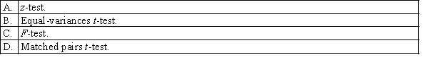
سؤال
A sample of size 300 had 96 successes. The lower limit of the 99% confidence interval for the population proportion is: 
سؤال
For a sample of size 25 observations taken from a normally distributed population. The sample standard deviation is 6, a 95% confidence interval estimate for the population mean would require the use of: 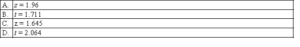
سؤال
Two independent samples of sizes 50 and 50 are randomly selected from two populations to test the difference between the population means,  . The sampling distribution of the sample mean difference
  is:
is: 
. The sampling distribution of the sample mean difference is: سؤال
In testing the hypotheses: 
 , suppose the p-value is 0.03. Which of the following is correct?
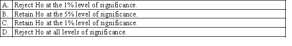
, suppose the p-value is 0.03. Which of the following is correct? سؤال
In a hypothesis test for the population variance, the hypotheses are:  .
.  . If the sample size is 15 and the test is being carried out at the 5% level of significance, the null hypothesis will be rejected if:
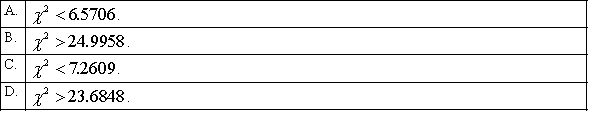
. . If the sample size is 15 and the test is being carried out at the 5% level of significance, the null hypothesis will be rejected if: سؤال
Two independent samples of sizes 20 and 25 are randomly selected from two normal populations with equal variances. In order to test the difference between the population means, the test statistic is: 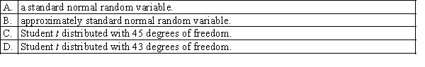
سؤال
Assuming that all necessary conditions are met, what needs to be changed in the formula 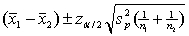 so that we can use it to construct a confidence interval estimate for the difference of two population means when the population variances are assumed to be equal?
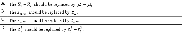
so that we can use it to construct a confidence interval estimate for the difference of two population means when the population variances are assumed to be equal? سؤال
Which of the following statements is correct regarding the percentile points of the F-distribution? 
سؤال
سؤال
سؤال
A sample of size 200 from population 1 has 50 successes. A sample of size 200 from population 2 has 40 successes. The value of the test statistic for testing the null hypothesis that the proportion of successes in population 1 exceeds the proportion of successes in population 2 by 0.025 is: 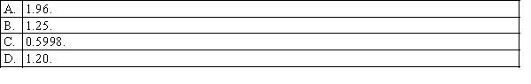
سؤال
When the necessary conditions are met, a two-tail test is being conducted to test the difference between two population proportions, testing at the 5% level of significance. Which of the following is the p-value for this test if the calculated z test statistic is 1.34? 
سؤال
In testing for the equality of two population variances, when the populations are normally distributed, the 5% level of significance has been used. To determine the rejection region, it will be necessary to refer to the F table corresponding to an upper-tail area of: 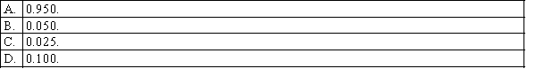
سؤال
A random sample of 20 observations taken from a normally distributed population revealed a sample mean of 65 and a sample variance of 16. The lower limit of a 90% confidence interval for the population mean would equal: 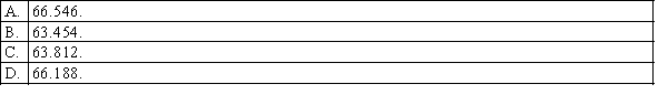
سؤال
In testing the difference between two population means using two independent samples, the population standard deviations are assumed to be known and the calculated test statistic equals 1.05. If the test is upper-tail and the 10% level of significance has been specified, the conclusion should be to: 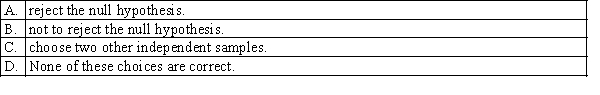
سؤال
When the necessary conditions are met, a two-tail test is being conducted to test the difference between two population proportions, but your statistical software provides only a one-tail area of 0.03 as part of its output. The p-value for this test will be: 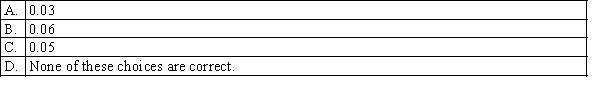
سؤال
After calculating the sample size needed to estimate a population proportion to within 0.05, you have been told that the maximum allowable error must be reduced to just 0.025. If the original calculation led to a sample size of 1000, the sample size will now have to be: 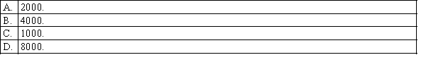
سؤال
A random sample of size 15 taken from a normally distributed population resulted in a sample variance of 25. The upper limit of a 99% confidence interval for the population variance would be: 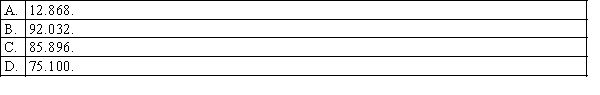
سؤال
سؤال
In a hypothesis test for the population variance, the hypotheses are: 
 If the sample size is 25 and the test is being carried out at the 5% level of significance, the rejection region will be:
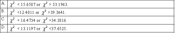
If the sample size is 25 and the test is being carried out at the 5% level of significance, the rejection region will be: سؤال
سؤال
سؤال
Two samples of sizes 22 and 18 are independently drawn from two normal populations, where the unknown population variances are assumed to be equal. The number of degrees of freedom of the equal-variances t-test statistic is: 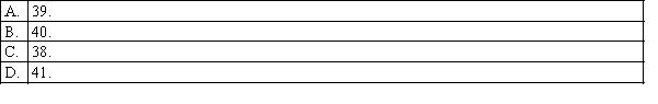
سؤال
From a sample of 500 items, 30 were found to be defective. The point estimate of the population proportion defective will be: 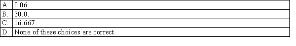
سؤال
سؤال
For a sample of 25 observations taken from a normally distributed population with standard deviation of 6, a 95% confidence interval estimate for the population mean would require the use of: 
سؤال
A sample of size 125 selected from one population has 55 successes, and a sample of size 140 selected from a second population has 70 successes. The test statistic for testing the equality of the population proportions is equal to: 
سؤال
In constructing a 90% confidence interval estimate for the difference between the means of two normally distributed populations, where the unknown population variances are assumed not to be equal, summary statistics computed from two independent samples are as follows:  ,
,  ,
,  .
.  ,
,  ,
,  . The lower confidence limit is:
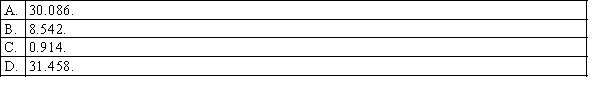
, , . , , . The lower confidence limit is: سؤال
Which of the following is the number of degrees of freedom associated with the t-test, when the data are gathered from a matched pairs experiment with 30 pairs? 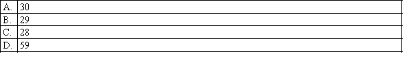
سؤال
In testing whether the means of two normal populations are equal, summary statistics computed for two independent samples are as follows:  ,
,  ,
,  .
.  ,
,  ,
,  . Assume that the population variances are unequal. The standard error of the sampling distribution of the sample mean difference
  is equal to:
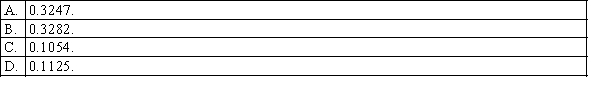
, , . , , . Assume that the population variances are unequal. The standard error of the sampling distribution of the sample mean difference is equal to: سؤال
In constructing a 95% interval estimate for the ratio of two population variances,  /
/  , two independent samples of sizes 30 and 40 are drawn from the populations. If the sample variances are 425 and 675, then the upper confidence limit is about:
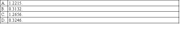
/ , two independent samples of sizes 30 and 40 are drawn from the populations. If the sample variances are 425 and 675, then the upper confidence limit is about: سؤال
سؤال
A random sample of 30 observations is selected from a normally distributed population. The sample variance is 12. In the 90% confidence interval for the population variance, the upper limit will be: 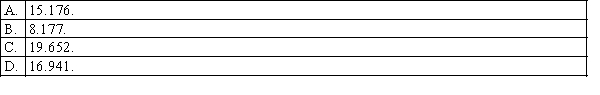
سؤال
In testing the hypotheses: 
 , at the 10% significance level, if the sample proportion is 0.56, and the standard error of the sample proportion is 0.025, the appropriate conclusion is:
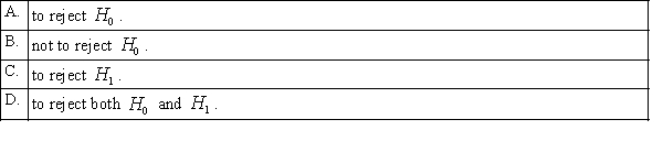
, at the 10% significance level, if the sample proportion is 0.56, and the standard error of the sample proportion is 0.025, the appropriate conclusion is: سؤال
Which of the following is a required condition for using the normal approximation to the binomial in constructing interval estimate for the difference between two population proportions? 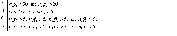
سؤال
Two independent samples of sizes 35 and 40 are randomly selected from two normally distributed populations. Assume that the population variances are unknown but equal. In order to test the difference between the population means,  , the sampling distribution of the sample mean difference,
  , is:
, is: 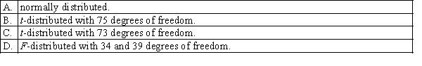
, the sampling distribution of the sample mean difference, , is: سؤال
Suppose that a one-tail t-test is being applied to find out if the population mean is at least 80. The level of significance is 0.10 and 25 observations were sampled. The rejection region is: 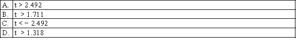
سؤال
When the necessary conditions are met, a one-tail test is being conducted to test the difference between two population proportions, but your statistical software provides only a two-tail area of 0.058 as part of its output. The p-value for this test will be: 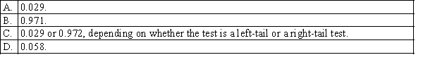
سؤال
سؤال
سؤال
سؤال
سؤال
سؤال
سؤال
سؤال
سؤال
سؤال
سؤال
سؤال
سؤال
سؤال
سؤال
سؤال
سؤال
سؤال
سؤال
سؤال
سؤال
سؤال
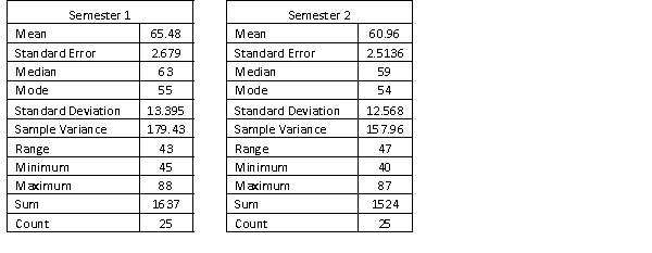
A statistics course at a large university is taught in each semester. A student has noticed that the students in semester 1 and semester 2 are enrolled in different degrees. To investigate, the student takes a random sample of 25 students from semester 1 and 25 students from semester 2 and records their final marks (%) provided in the table below. Excel was used to generate descriptive statistics on each sample.
Assume that student final marks are normally distributed in each semester.
 Estimate and interpret a 95% confidence interval for the proportion of semester 2 students that passed the course.
Assume that student final marks are normally distributed in each semester.
Estimate and interpret a 95% confidence interval for the proportion of semester 2 students that passed the course. سؤال
سؤال
سؤال
A statistics course at a large university is taught in each semester. A student has noticed that the students in semester 1 and semester 2 are enrolled in different degrees. To investigate, the student takes a random sample of 25 students from semester 1 and 25 students from semester 2 and records their final marks (%) provided in the table below. Excel was used to generate descriptive statistics on each sample.
Assume that student final marks are normally distributed in each semester.
 (a) Can we conclude at the 5% level of significance that over 40% of students in the population scored a pass grade in semester 1, where a pass grade is 50% to 64%?
(b) Find the p-value of the test and briefly explain how to use it to test the hypotheses.
Assume that student final marks are normally distributed in each semester.
(a) Can we conclude at the 5% level of significance that over 40% of students in the population scored a pass grade in semester 1, where a pass grade is 50% to 64%?(b) Find the p-value of the test and briefly explain how to use it to test the hypotheses.
سؤال
سؤال
سؤال
سؤال
A statistics course at a large university is taught in each semester. A student has noticed that the students in semester 1 and semester 2 are enrolled in different degrees. To investigate, the student takes a random sample of 25 students from semester 1 and 25 students from semester 2 and records their final marks (%) provided in the table below. Excel was used to generate descriptive statistics on each sample.
Assume that student final marks are normally distributed in each semester.
 Estimate a 95% confidence interval for the difference in final marks between semester 1
and semester 2 students in this statistics course. Assume that the population variances are unknown
and equal.
Assume that student final marks are normally distributed in each semester.
Estimate a 95% confidence interval for the difference in final marks between semester 1and semester 2 students in this statistics course. Assume that the population variances are unknown
and equal.
سؤال
A statistics course at a large university is taught in each semester. A student has noticed that the students in semester 1 and semester 2 are enrolled in different degrees. To investigate, the student takes a random sample of 25 students from semester 1 and 25 students from semester 2 and records their final marks (%) provided in the table below. Excel was used to generate descriptive statistics on each sample.
Assume that student final marks are normally distributed in each semester.
 (a) Can we conclude at the 5% level of significance that semester 1 students have a higher proportion of high distinctions than semester 2 students, where a high distinction is a final mark greater than or equal to 85%?
(b) Find the p-value of the test, and explain how to use it to test the hypotheses.
Assume that student final marks are normally distributed in each semester.
(a) Can we conclude at the 5% level of significance that semester 1 students have a higher proportion of high distinctions than semester 2 students, where a high distinction is a final mark greater than or equal to 85%?(b) Find the p-value of the test, and explain how to use it to test the hypotheses.
سؤال
A statistics course at a large university is taught in each semester. A student has noticed that the students in semester 1 and semester 2 are enrolled in different degrees. To investigate, the student takes a random sample of 25 students from semester 1 and 25 students from semester 2 and records their final marks (%) provided in the table below. Excel was used to generate descriptive statistics on each sample.
Assume that student final marks are normally distributed in each semester.
 Estimate and interpret a 95% confidence interval for the population average final mark for semester 2 students.
Assume that student final marks are normally distributed in each semester.
Estimate and interpret a 95% confidence interval for the population average final mark for semester 2 students. سؤال
سؤال
سؤال
سؤال
سؤال
سؤال
سؤال
سؤال
سؤال
A statistics course at a large university is taught in each semester. A student has noticed that the students in semester 1 and semester 2 are enrolled in different degrees. To investigate, the student takes a random sample of 25 students from semester 1 and 25 students from semester 2 and records their final marks (%) provided in the table below. Excel was used to generate descriptive statistics on each sample.
Assume that student final marks are normally distributed in each semester.
 Estimate and interpret a 95% confidence interval for the population average final mark for semester 1 students.
Assume that student final marks are normally distributed in each semester.
Estimate and interpret a 95% confidence interval for the population average final mark for semester 1 students. سؤال
A statistics course at a large university is taught in each semester. A student has noticed that the students in semester 1 and semester 2 are enrolled in different degrees. To investigate, the student takes a random sample of 25 students from semester 1 and 25 students from semester 2 and records their final marks (%) provided in the table below. Excel was used to generate descriptive statistics on each sample.
Assume that student final marks are normally distributed in each semester.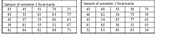
 Estimate a 95% confidence interval for the difference in the proportions of students who received a high distinction in semester 1 to semester 2.
Assume that student final marks are normally distributed in each semester.
Estimate a 95% confidence interval for the difference in the proportions of students who received a high distinction in semester 1 to semester 2.
فتح الحزمة
قم بالتسجيل لفتح البطاقات في هذه المجموعة!
Unlock Deck
Unlock Deck
1/106
العب
ملء الشاشة (f)
Deck 22: Statistical Inference: Conclusion
1
In testing the difference between two population means for which the population variances are unknown and assumed to be equal, two independent samples are drawn from the populations. Which of the following tests is appropriate?
B
2
A sample of size 300 had 96 successes. The lower limit of the 99% confidence interval for the population proportion is:
C
3
For a sample of size 25 observations taken from a normally distributed population. The sample standard deviation is 6, a 95% confidence interval estimate for the population mean would require the use of:
D
4
Two independent samples of sizes 50 and 50 are randomly selected from two populations to test the difference between the population means, . The sampling distribution of the sample mean difference is:
. The sampling distribution of the sample mean difference is: فتح الحزمة
افتح القفل للوصول البطاقات البالغ عددها 106 في هذه المجموعة.
فتح الحزمة
k this deck
5
In testing the hypotheses: , suppose the p-value is 0.03. Which of the following is correct?
, suppose the p-value is 0.03. Which of the following is correct? فتح الحزمة
افتح القفل للوصول البطاقات البالغ عددها 106 في هذه المجموعة.
فتح الحزمة
k this deck
6
In a hypothesis test for the population variance, the hypotheses are: . . If the sample size is 15 and the test is being carried out at the 5% level of significance, the null hypothesis will be rejected if:
. . If the sample size is 15 and the test is being carried out at the 5% level of significance, the null hypothesis will be rejected if: فتح الحزمة
افتح القفل للوصول البطاقات البالغ عددها 106 في هذه المجموعة.
فتح الحزمة
k this deck
7
Two independent samples of sizes 20 and 25 are randomly selected from two normal populations with equal variances. In order to test the difference between the population means, the test statistic is:
فتح الحزمة
افتح القفل للوصول البطاقات البالغ عددها 106 في هذه المجموعة.
فتح الحزمة
k this deck
8
Assuming that all necessary conditions are met, what needs to be changed in the formula so that we can use it to construct a confidence interval estimate for the difference of two population means when the population variances are assumed to be equal?
so that we can use it to construct a confidence interval estimate for the difference of two population means when the population variances are assumed to be equal? فتح الحزمة
افتح القفل للوصول البطاقات البالغ عددها 106 في هذه المجموعة.
فتح الحزمة
k this deck
9
Which of the following statements is correct regarding the percentile points of the F-distribution?
فتح الحزمة
افتح القفل للوصول البطاقات البالغ عددها 106 في هذه المجموعة.
فتح الحزمة
k this deck
10
When the necessary conditions are met, a two-tail test is being conducted to test the difference between two population proportions. The two sample proportions are = 0.21 and = 0.15, and the standard error of the sampling distribution of are - is 0.018. The calculated value of the test statistic will be:
فتح الحزمة
افتح القفل للوصول البطاقات البالغ عددها 106 في هذه المجموعة.
فتح الحزمة
k this deck
11
In testing the null hypothesis , if is false, the test could lead to:
فتح الحزمة
افتح القفل للوصول البطاقات البالغ عددها 106 في هذه المجموعة.
فتح الحزمة
k this deck
12
A sample of size 200 from population 1 has 50 successes. A sample of size 200 from population 2 has 40 successes. The value of the test statistic for testing the null hypothesis that the proportion of successes in population 1 exceeds the proportion of successes in population 2 by 0.025 is:
فتح الحزمة
افتح القفل للوصول البطاقات البالغ عددها 106 في هذه المجموعة.
فتح الحزمة
k this deck
13
When the necessary conditions are met, a two-tail test is being conducted to test the difference between two population proportions, testing at the 5% level of significance. Which of the following is the p-value for this test if the calculated z test statistic is 1.34?
فتح الحزمة
افتح القفل للوصول البطاقات البالغ عددها 106 في هذه المجموعة.
فتح الحزمة
k this deck
14
In testing for the equality of two population variances, when the populations are normally distributed, the 5% level of significance has been used. To determine the rejection region, it will be necessary to refer to the F table corresponding to an upper-tail area of:
فتح الحزمة
افتح القفل للوصول البطاقات البالغ عددها 106 في هذه المجموعة.
فتح الحزمة
k this deck
15
A random sample of 20 observations taken from a normally distributed population revealed a sample mean of 65 and a sample variance of 16. The lower limit of a 90% confidence interval for the population mean would equal:
فتح الحزمة
افتح القفل للوصول البطاقات البالغ عددها 106 في هذه المجموعة.
فتح الحزمة
k this deck
16
In testing the difference between two population means using two independent samples, the population standard deviations are assumed to be known and the calculated test statistic equals 1.05. If the test is upper-tail and the 10% level of significance has been specified, the conclusion should be to:
فتح الحزمة
افتح القفل للوصول البطاقات البالغ عددها 106 في هذه المجموعة.
فتح الحزمة
k this deck
17
When the necessary conditions are met, a two-tail test is being conducted to test the difference between two population proportions, but your statistical software provides only a one-tail area of 0.03 as part of its output. The p-value for this test will be:
فتح الحزمة
افتح القفل للوصول البطاقات البالغ عددها 106 في هذه المجموعة.
فتح الحزمة
k this deck
18
After calculating the sample size needed to estimate a population proportion to within 0.05, you have been told that the maximum allowable error must be reduced to just 0.025. If the original calculation led to a sample size of 1000, the sample size will now have to be:
فتح الحزمة
افتح القفل للوصول البطاقات البالغ عددها 106 في هذه المجموعة.
فتح الحزمة
k this deck
19
A random sample of size 15 taken from a normally distributed population resulted in a sample variance of 25. The upper limit of a 99% confidence interval for the population variance would be:
فتح الحزمة
افتح القفل للوصول البطاقات البالغ عددها 106 في هذه المجموعة.
فتح الحزمة
k this deck
20
Based on sample data, the 95% confidence interval limits for the population mean are LCL = 124.6 and UCL = 148.2. If the 5% level of significance were used in testing the hypotheses:
H0 : = 150
H1 : 150,
The null hypothesis:
H0 : = 150
H1 : 150,
The null hypothesis:
فتح الحزمة
افتح القفل للوصول البطاقات البالغ عددها 106 في هذه المجموعة.
فتح الحزمة
k this deck
21
In a hypothesis test for the population variance, the hypotheses are: If the sample size is 25 and the test is being carried out at the 5% level of significance, the rejection region will be:
If the sample size is 25 and the test is being carried out at the 5% level of significance, the rejection region will be: فتح الحزمة
افتح القفل للوصول البطاقات البالغ عددها 106 في هذه المجموعة.
فتح الحزمة
k this deck
22
In testing the hypotheses: H0 : = 140
H1 : 140,
Suppose that we rejected the null hypothesis at = 0.10. Then for which of the following ? values do we also reject the null hypothesis?
H1 : 140,
Suppose that we rejected the null hypothesis at = 0.10. Then for which of the following ? values do we also reject the null hypothesis?
فتح الحزمة
افتح القفل للوصول البطاقات البالغ عددها 106 في هذه المجموعة.
فتح الحزمة
k this deck
23
The pooled-variance estimator, , requires that the two population variances be equal.
فتح الحزمة
افتح القفل للوصول البطاقات البالغ عددها 106 في هذه المجموعة.
فتح الحزمة
k this deck
24
Two samples of sizes 22 and 18 are independently drawn from two normal populations, where the unknown population variances are assumed to be equal. The number of degrees of freedom of the equal-variances t-test statistic is:
فتح الحزمة
افتح القفل للوصول البطاقات البالغ عددها 106 في هذه المجموعة.
فتح الحزمة
k this deck
25
From a sample of 500 items, 30 were found to be defective. The point estimate of the population proportion defective will be:
فتح الحزمة
افتح القفل للوصول البطاقات البالغ عددها 106 في هذه المجموعة.
فتح الحزمة
k this deck
26
Which of the following best describes a p-value?
فتح الحزمة
افتح القفل للوصول البطاقات البالغ عددها 106 في هذه المجموعة.
فتح الحزمة
k this deck
27
For a sample of 25 observations taken from a normally distributed population with standard deviation of 6, a 95% confidence interval estimate for the population mean would require the use of:
فتح الحزمة
افتح القفل للوصول البطاقات البالغ عددها 106 في هذه المجموعة.
فتح الحزمة
k this deck
28
A sample of size 125 selected from one population has 55 successes, and a sample of size 140 selected from a second population has 70 successes. The test statistic for testing the equality of the population proportions is equal to:
فتح الحزمة
افتح القفل للوصول البطاقات البالغ عددها 106 في هذه المجموعة.
فتح الحزمة
k this deck
29
In constructing a 90% confidence interval estimate for the difference between the means of two normally distributed populations, where the unknown population variances are assumed not to be equal, summary statistics computed from two independent samples are as follows: , , . , , . The lower confidence limit is:
, , . , , . The lower confidence limit is: فتح الحزمة
افتح القفل للوصول البطاقات البالغ عددها 106 في هذه المجموعة.
فتح الحزمة
k this deck
30
Which of the following is the number of degrees of freedom associated with the t-test, when the data are gathered from a matched pairs experiment with 30 pairs?
فتح الحزمة
افتح القفل للوصول البطاقات البالغ عددها 106 في هذه المجموعة.
فتح الحزمة
k this deck
31
In testing whether the means of two normal populations are equal, summary statistics computed for two independent samples are as follows: , , . , , . Assume that the population variances are unequal. The standard error of the sampling distribution of the sample mean difference is equal to:
, , . , , . Assume that the population variances are unequal. The standard error of the sampling distribution of the sample mean difference is equal to: فتح الحزمة
افتح القفل للوصول البطاقات البالغ عددها 106 في هذه المجموعة.
فتح الحزمة
k this deck
32
In constructing a 95% interval estimate for the ratio of two population variances, / , two independent samples of sizes 30 and 40 are drawn from the populations. If the sample variances are 425 and 675, then the upper confidence limit is about:
/ , two independent samples of sizes 30 and 40 are drawn from the populations. If the sample variances are 425 and 675, then the upper confidence limit is about: فتح الحزمة
افتح القفل للوصول البطاقات البالغ عددها 106 في هذه المجموعة.
فتح الحزمة
k this deck
33
When comparing two population variances, we test H0: = 0.
فتح الحزمة
افتح القفل للوصول البطاقات البالغ عددها 106 في هذه المجموعة.
فتح الحزمة
k this deck
34
A random sample of 30 observations is selected from a normally distributed population. The sample variance is 12. In the 90% confidence interval for the population variance, the upper limit will be:
فتح الحزمة
افتح القفل للوصول البطاقات البالغ عددها 106 في هذه المجموعة.
فتح الحزمة
k this deck
35
In testing the hypotheses: , at the 10% significance level, if the sample proportion is 0.56, and the standard error of the sample proportion is 0.025, the appropriate conclusion is:
, at the 10% significance level, if the sample proportion is 0.56, and the standard error of the sample proportion is 0.025, the appropriate conclusion is: فتح الحزمة
افتح القفل للوصول البطاقات البالغ عددها 106 في هذه المجموعة.
فتح الحزمة
k this deck
36
Which of the following is a required condition for using the normal approximation to the binomial in constructing interval estimate for the difference between two population proportions?
فتح الحزمة
افتح القفل للوصول البطاقات البالغ عددها 106 في هذه المجموعة.
فتح الحزمة
k this deck
37
Two independent samples of sizes 35 and 40 are randomly selected from two normally distributed populations. Assume that the population variances are unknown but equal. In order to test the difference between the population means, , the sampling distribution of the sample mean difference, , is:
, the sampling distribution of the sample mean difference, , is: فتح الحزمة
افتح القفل للوصول البطاقات البالغ عددها 106 في هذه المجموعة.
فتح الحزمة
k this deck
38
Suppose that a one-tail t-test is being applied to find out if the population mean is at least 80. The level of significance is 0.10 and 25 observations were sampled. The rejection region is:
فتح الحزمة
افتح القفل للوصول البطاقات البالغ عددها 106 في هذه المجموعة.
فتح الحزمة
k this deck
39
When the necessary conditions are met, a one-tail test is being conducted to test the difference between two population proportions, but your statistical software provides only a two-tail area of 0.058 as part of its output. The p-value for this test will be:
فتح الحزمة
افتح القفل للوصول البطاقات البالغ عددها 106 في هذه المجموعة.
فتح الحزمة
k this deck
40
If we reject a null hypothesis at the 0.05 level of significance, then we must also reject it at the 0.10 level.
فتح الحزمة
افتح القفل للوصول البطاقات البالغ عددها 106 في هذه المجموعة.
فتح الحزمة
k this deck
41
If a sample of size 28 is selected, the value of A for the probability P(-A tdf=n-1 t A) = 0.99 is 2.771.
فتح الحزمة
افتح القفل للوصول البطاقات البالغ عددها 106 في هذه المجموعة.
فتح الحزمة
k this deck
42
If a null hypothesis about the population proportion p is rejected at the 0.05 level of significance, it must be rejected at the 0.01 level.
فتح الحزمة
افتح القفل للوصول البطاقات البالغ عددها 106 في هذه المجموعة.
فتح الحزمة
k this deck
43
If a sample has 20 observations and a 95% confidence estimate for is needed, the appropriate t-score is 1.729.
فتح الحزمة
افتح القفل للوصول البطاقات البالغ عددها 106 في هذه المجموعة.
فتح الحزمة
k this deck
44
We use the F-test to determine whether two population variances are equal.
فتح الحزمة
افتح القفل للوصول البطاقات البالغ عددها 106 في هذه المجموعة.
فتح الحزمة
k this deck
45
The lower limit of the 87.4% confidence interval for the population proportion p, given that n = 250 and = 0.15, is 0.1492.
فتح الحزمة
افتح القفل للوصول البطاقات البالغ عددها 106 في هذه المجموعة.
فتح الحزمة
k this deck
46
Both the equal-variances and unequal-variances t-test statistics of require that the two populations be Student t-distributed.
فتح الحزمة
افتح القفل للوصول البطاقات البالغ عددها 106 في هذه المجموعة.
فتح الحزمة
k this deck
47
When the necessary conditions are met, a two-tail test is being conducted to test the difference between two population proportions. If the value of the test statistic z is 1.53, then the p-value is 0.126.
فتح الحزمة
افتح القفل للوصول البطاقات البالغ عددها 106 في هذه المجموعة.
فتح الحزمة
k this deck
48
The number of degrees of freedom associated with the t-test, when the data are gathered from a matched pairs experiment with 8 pairs, is 14.
فتح الحزمة
افتح القفل للوصول البطاقات البالغ عددها 106 في هذه المجموعة.
فتح الحزمة
k this deck
49
When the necessary conditions are met, a two-tail test is being conducted to test the difference between two population means, but your statistical software provides only a one-tail area of 0.0327 as part of its output. The p-value for this test will be 0.0654.
فتح الحزمة
افتح القفل للوصول البطاقات البالغ عددها 106 في هذه المجموعة.
فتح الحزمة
k this deck
50
If a sample has 300 observations and a 97.5% confidence estimate for p is needed, the appropriate z-score is 2.24.
فتح الحزمة
افتح القفل للوصول البطاقات البالغ عددها 106 في هذه المجموعة.
فتح الحزمة
k this deck
51
If a sample of size 300 is selected, the value of A for the probability P(-A tdf=n-1 A) = 0.90 is 1.96.
فتح الحزمة
افتح القفل للوصول البطاقات البالغ عددها 106 في هذه المجموعة.
فتح الحزمة
k this deck
52
When the necessary conditions are met, a two-tail test is being conducted to test the difference between two population proportions. The two sample proportions are = 0.32 and = 0.38, and the standard error of the sampling distribution of is 0.046. The calculated value of the test statistic will be 1.3043.
فتح الحزمة
افتح القفل للوصول البطاقات البالغ عددها 106 في هذه المجموعة.
فتح الحزمة
k this deck
53
Two samples of size 30 each are independently drawn from two normal populations, where the unknown population variances are assumed to be equal. The number of degrees of freedom of the equal-variances t-test statistic is 59.
فتح الحزمة
افتح القفل للوصول البطاقات البالغ عددها 106 في هذه المجموعة.
فتح الحزمة
k this deck
54
If a sample of size 25 is selected, the value of A for the probability P(tdf=n-1 A) = 0.05 is 1.708.
فتح الحزمة
افتح القفل للوصول البطاقات البالغ عددها 106 في هذه المجموعة.
فتح الحزمة
k this deck
55
The upper limit of the 89.9% confidence interval for the population proportion p, given that n = 80 and = 0.40, is 0.4898.
فتح الحزمة
افتح القفل للوصول البطاقات البالغ عددها 106 في هذه المجموعة.
فتح الحزمة
k this deck
56
If a sample has 25 observations and a 99% confidence estimate for is needed, the appropriate t-score is 2.797.
فتح الحزمة
افتح القفل للوصول البطاقات البالغ عددها 106 في هذه المجموعة.
فتح الحزمة
k this deck
57
In a one-tail test, the p-value is found to be equal to 0.0456. If the test had been two-tailed, the p-value would have been 0.0912.
فتح الحزمة
افتح القفل للوصول البطاقات البالغ عددها 106 في هذه المجموعة.
فتح الحزمة
k this deck
58
A one-tail test of the population proportion produces a test statistic z = -2.12. The p-value of the test is 0.034.
فتح الحزمة
افتح القفل للوصول البطاقات البالغ عددها 106 في هذه المجموعة.
فتح الحزمة
k this deck
59
When the necessary conditions are met, a two-tail test is being conducted at = 0.10 to test H0: = 1. The two sample variances are = 736 and = 1024, and the sample sizes are n1 = 16 and n2 = 25. The rejection region is F > 2.11 or F < 0.4367.
فتح الحزمة
افتح القفل للوصول البطاقات البالغ عددها 106 في هذه المجموعة.
فتح الحزمة
k this deck
60
When the necessary conditions are met, a two-tail test is being conducted at = 0.025 to test
H0: = 1. The two sample variances are = 375 and = 625, and the sample sizes are
n1 = 36 and n2 = 36. The calculated value of the test statistic will be F = 0.60.
H0: = 1. The two sample variances are = 375 and = 625, and the sample sizes are
n1 = 36 and n2 = 36. The calculated value of the test statistic will be F = 0.60.
فتح الحزمة
افتح القفل للوصول البطاقات البالغ عددها 106 في هذه المجموعة.
فتح الحزمة
k this deck
61
A statistics course at a large university is taught in each semester. A student has noticed that the students in semester 1 and semester 2 are enrolled in different degrees. To investigate, the student takes a random sample of 25 students from semester 1 and 25 students from semester 2 and records their final marks (%) provided in the table below. Excel was used to generate descriptive statistics on each sample.
Assume that student final marks are normally distributed in each semester. Estimate and interpret a 95% confidence interval for the proportion of semester 2 students that passed the course.
Assume that student final marks are normally distributed in each semester.
Estimate and interpret a 95% confidence interval for the proportion of semester 2 students that passed the course. فتح الحزمة
افتح القفل للوصول البطاقات البالغ عددها 106 في هذه المجموعة.
فتح الحزمة
k this deck
62
A statistics course at a large university is taught in each semester. A student has noticed that the students in semester 1 and semester 2 are enrolled in different degrees. To investigate, the student takes a random sample of 25 students from semester 1 and 25 students from semester 2 and records their final marks (%) provided in the table below. Excel was used to generate descriptive statistics on each sample.
Assume that student final marks are normally distributed in each semester. (a) Determine whether these data are sufficient to infer at the 10% level of significance that the two population variances differ.
(b) Explain the decision of your test in part (a) in the context of this question.
Assume that student final marks are normally distributed in each semester. (a) Determine whether these data are sufficient to infer at the 10% level of significance that the two population variances differ.
(b) Explain the decision of your test in part (a) in the context of this question.
فتح الحزمة
افتح القفل للوصول البطاقات البالغ عددها 106 في هذه المجموعة.
فتح الحزمة
k this deck
63
The irradiation of food to destroy bacteria is an increasingly common practice. In order to determine which one of two methods of irradiation is best, a scientist took a random sample of 100 one-kilogram packages of minced meat and subjected 50 of them to irradiation method 1 and the remaining 50 to irradiation method 2. The bacteria counts were measured and the following statistics were computed. The scientist noted that the data were normally distributed. Determine whether these data are sufficient to infer at the 5% significance level that the two population variances differ.
فتح الحزمة
افتح القفل للوصول البطاقات البالغ عددها 106 في هذه المجموعة.
فتح الحزمة
k this deck
64
A statistics course at a large university is taught in each semester. A student has noticed that the students in semester 1 and semester 2 are enrolled in different degrees. To investigate, the student takes a random sample of 25 students from semester 1 and 25 students from semester 2 and records their final marks (%) provided in the table below. Excel was used to generate descriptive statistics on each sample.
Assume that student final marks are normally distributed in each semester. (a) Can we conclude at the 5% level of significance that over 40% of students in the population scored a pass grade in semester 1, where a pass grade is 50% to 64%?
(b) Find the p-value of the test and briefly explain how to use it to test the hypotheses.
Assume that student final marks are normally distributed in each semester.
(a) Can we conclude at the 5% level of significance that over 40% of students in the population scored a pass grade in semester 1, where a pass grade is 50% to 64%?(b) Find the p-value of the test and briefly explain how to use it to test the hypotheses.
فتح الحزمة
افتح القفل للوصول البطاقات البالغ عددها 106 في هذه المجموعة.
فتح الحزمة
k this deck
65
Descriptive statistics helps us describe and summarise data whereas inferential statistics helps us draw conclusions about populations based on samples of data.
فتح الحزمة
افتح القفل للوصول البطاقات البالغ عددها 106 في هذه المجموعة.
فتح الحزمة
k this deck
66
With hypothesis testing, there are only two types of errors: Type I error where we incorrectly reject Ho and Type II error where we incorrectly retain Ho.
فتح الحزمة
افتح القفل للوصول البطاقات البالغ عددها 106 في هذه المجموعة.
فتح الحزمة
k this deck
67
The equal-variances test statistic of is Student t-distributed with n1 + n2 - 2 degrees of freedom, provided that the two sample sizes are equal.
فتح الحزمة
افتح القفل للوصول البطاقات البالغ عددها 106 في هذه المجموعة.
فتح الحزمة
k this deck
68
A statistics course at a large university is taught in each semester. A student has noticed that the students in semester 1 and semester 2 are enrolled in different degrees. To investigate, the student takes a random sample of 25 students from semester 1 and 25 students from semester 2 and records their final marks (%) provided in the table below. Excel was used to generate descriptive statistics on each sample.
Assume that student final marks are normally distributed in each semester. Estimate a 95% confidence interval for the difference in final marks between semester 1
and semester 2 students in this statistics course. Assume that the population variances are unknown
and equal.
Assume that student final marks are normally distributed in each semester.
Estimate a 95% confidence interval for the difference in final marks between semester 1and semester 2 students in this statistics course. Assume that the population variances are unknown
and equal.
فتح الحزمة
افتح القفل للوصول البطاقات البالغ عددها 106 في هذه المجموعة.
فتح الحزمة
k this deck
69
A statistics course at a large university is taught in each semester. A student has noticed that the students in semester 1 and semester 2 are enrolled in different degrees. To investigate, the student takes a random sample of 25 students from semester 1 and 25 students from semester 2 and records their final marks (%) provided in the table below. Excel was used to generate descriptive statistics on each sample.
Assume that student final marks are normally distributed in each semester. (a) Can we conclude at the 5% level of significance that semester 1 students have a higher proportion of high distinctions than semester 2 students, where a high distinction is a final mark greater than or equal to 85%?
(b) Find the p-value of the test, and explain how to use it to test the hypotheses.
Assume that student final marks are normally distributed in each semester.
(a) Can we conclude at the 5% level of significance that semester 1 students have a higher proportion of high distinctions than semester 2 students, where a high distinction is a final mark greater than or equal to 85%?(b) Find the p-value of the test, and explain how to use it to test the hypotheses.
فتح الحزمة
افتح القفل للوصول البطاقات البالغ عددها 106 في هذه المجموعة.
فتح الحزمة
k this deck
70
A statistics course at a large university is taught in each semester. A student has noticed that the students in semester 1 and semester 2 are enrolled in different degrees. To investigate, the student takes a random sample of 25 students from semester 1 and 25 students from semester 2 and records their final marks (%) provided in the table below. Excel was used to generate descriptive statistics on each sample.
Assume that student final marks are normally distributed in each semester. Estimate and interpret a 95% confidence interval for the population average final mark for semester 2 students.
Assume that student final marks are normally distributed in each semester.
Estimate and interpret a 95% confidence interval for the population average final mark for semester 2 students. فتح الحزمة
افتح القفل للوصول البطاقات البالغ عددها 106 في هذه المجموعة.
فتح الحزمة
k this deck
71
A statistics course at a large university is taught in each semester. A student has noticed that the students in semester 1 and semester 2 are enrolled in different degrees. To investigate, the student takes a random sample of 25 students from semester 1 and 25 students from semester 2 and records their final marks (%) provided in the table below. Excel was used to generate descriptive statistics on each sample.
Assume that student final marks are normally distributed in each semester. There is a rumor going around the university that students with a higher IQ are enrolled in the semester 1 statistics course because they tend to be students enrolled in the degree with the higher entrance score for university. Can it be concluded at the 5% significance level that semester 1 students have a higher average final mark than semester 2 students? Assume that the population variances are unknown and equal.
Assume that student final marks are normally distributed in each semester. There is a rumor going around the university that students with a higher IQ are enrolled in the semester 1 statistics course because they tend to be students enrolled in the degree with the higher entrance score for university. Can it be concluded at the 5% significance level that semester 1 students have a higher average final mark than semester 2 students? Assume that the population variances are unknown and equal.
فتح الحزمة
افتح القفل للوصول البطاقات البالغ عددها 106 في هذه المجموعة.
فتح الحزمة
k this deck
72
A statistics course at a large university is taught in each semester. A student has noticed that the students in semester 1 and semester 2 are enrolled in different degrees. To investigate, the student takes a random sample of 25 students from semester 1 and 25 students from semester 2 and records their final marks (%) provided in the table below. Excel was used to generate descriptive statistics on each sample.
Assume that student final marks are normally distributed in each semester. Can we conclude at the 5% significance level that the variance of semester 2 student's final marks is greater than 150?
Assume that student final marks are normally distributed in each semester. Can we conclude at the 5% significance level that the variance of semester 2 student's final marks is greater than 150?
فتح الحزمة
افتح القفل للوصول البطاقات البالغ عددها 106 في هذه المجموعة.
فتح الحزمة
k this deck
73
The sampling distributions we use for nominal (categorical) data are the Standard Normal distribution and the Chi-squared distribution.
فتح الحزمة
افتح القفل للوصول البطاقات البالغ عددها 106 في هذه المجموعة.
فتح الحزمة
k this deck
74
If a sample has 12 observations and a 90% confidence estimate for µ is needed, the appropriate t-critical value from the t tables is 1.796.
فتح الحزمة
افتح القفل للوصول البطاقات البالغ عددها 106 في هذه المجموعة.
فتح الحزمة
k this deck
75
A statistics course at a large university is taught in each semester. A student has noticed that the students in semester 1 and semester 2 are enrolled in different degrees. To investigate, the student takes a random sample of 25 students from semester 1 and 25 students from semester 2 and records their final marks (%) provided in the table below. Excel was used to generate descriptive statistics on each sample.
Assume that student final marks are normally distributed in each semester. Can we conclude at the 5% significance level that the variance of semester 1 student's final marks is greater than 150?
Assume that student final marks are normally distributed in each semester. Can we conclude at the 5% significance level that the variance of semester 1 student's final marks is greater than 150?
فتح الحزمة
افتح القفل للوصول البطاقات البالغ عددها 106 في هذه المجموعة.
فتح الحزمة
k this deck
76
The sampling distributions we use for numerical data are the Standard Normal distribution, the Student's t-distribution and the F distribution.
فتح الحزمة
افتح القفل للوصول البطاقات البالغ عددها 106 في هذه المجموعة.
فتح الحزمة
k this deck
77
The sampling distribution of the random variable of interest is the source of statistical inference.
فتح الحزمة
افتح القفل للوصول البطاقات البالغ عددها 106 في هذه المجموعة.
فتح الحزمة
k this deck
78
A statistics course at a large university is taught in each semester. A student has noticed that the students in semester 1 and semester 2 are enrolled in different degrees. To investigate, the student takes a random sample of 25 students from semester 1 and 25 students from semester 2 and records their final marks (%) provided in the table below. Excel was used to generate descriptive statistics on each sample.
Assume that student final marks are normally distributed in each semester. Estimate and interpret a 90% confidence interval of the ratio of population variances of final student marks from semester 1 and semester 2.
Assume that student final marks are normally distributed in each semester. Estimate and interpret a 90% confidence interval of the ratio of population variances of final student marks from semester 1 and semester 2.
فتح الحزمة
افتح القفل للوصول البطاقات البالغ عددها 106 في هذه المجموعة.
فتح الحزمة
k this deck
79
A statistics course at a large university is taught in each semester. A student has noticed that the students in semester 1 and semester 2 are enrolled in different degrees. To investigate, the student takes a random sample of 25 students from semester 1 and 25 students from semester 2 and records their final marks (%) provided in the table below. Excel was used to generate descriptive statistics on each sample.
Assume that student final marks are normally distributed in each semester. Estimate and interpret a 95% confidence interval for the population average final mark for semester 1 students.
Assume that student final marks are normally distributed in each semester.
Estimate and interpret a 95% confidence interval for the population average final mark for semester 1 students. فتح الحزمة
افتح القفل للوصول البطاقات البالغ عددها 106 في هذه المجموعة.
فتح الحزمة
k this deck
80
A statistics course at a large university is taught in each semester. A student has noticed that the students in semester 1 and semester 2 are enrolled in different degrees. To investigate, the student takes a random sample of 25 students from semester 1 and 25 students from semester 2 and records their final marks (%) provided in the table below. Excel was used to generate descriptive statistics on each sample.
Assume that student final marks are normally distributed in each semester. Estimate a 95% confidence interval for the difference in the proportions of students who received a high distinction in semester 1 to semester 2.
Assume that student final marks are normally distributed in each semester.
Estimate a 95% confidence interval for the difference in the proportions of students who received a high distinction in semester 1 to semester 2. فتح الحزمة
افتح القفل للوصول البطاقات البالغ عددها 106 في هذه المجموعة.
فتح الحزمة
k this deck
فتح الحزمة
افتح القفل للوصول البطاقات البالغ عددها 106 في هذه المجموعة.


