Deck 8: Nonlinear Regression Functions
ملء الشاشة (f)
سؤال
An example of a quadratic regression model is 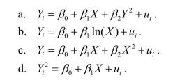
سؤال
سؤال
To decide whether 
fits the data better, you cannot consult the regression R2 because
A) ln (Y) may be negative for 0B) the TSS are not measured in the same units between the two models.
C) the slope no longer indicates the effect of a unit change of X on Y in the log-linear model.
D) the regression can be greater than one in the second model.
fits the data better, you cannot consult the regression R2 because
A) ln (Y) may be negative for 0
C) the slope no longer indicates the effect of a unit change of X on Y in the log-linear model.
D) the regression
can be greater than one in the second model. سؤال
The following interactions between binary and continuous variables are possible, with the exception of 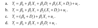
سؤال
A polynomial regression model is specified as: 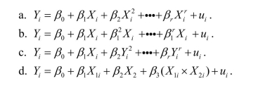
سؤال
سؤال
In nonlinear models, the expected change in the dependent variable for a change in one of the explanatory variables is given by 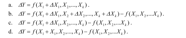
سؤال
سؤال
To test whether or not the population regression function is linear rather than a polynomial of order r, 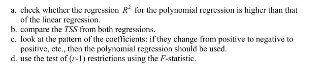
سؤال
سؤال
سؤال
سؤال
An example of the interaction term between two independent, continuous variables is 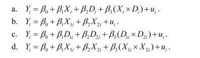
سؤال
The following are properties of the logarithm function with the exception of 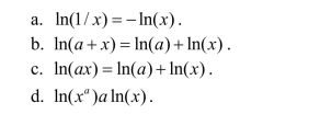
سؤال
You have estimated the following equation: 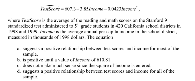
سؤال
سؤال
The exponential function 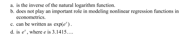
سؤال
سؤال
For the polynomial regression model, 
سؤال
سؤال
سؤال
سؤال
سؤال
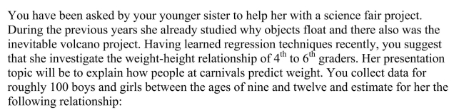
Suggest a transformation in the variables that will linearize the deterministic part of the
population regression functions below.Write the resulting regression function in a form
that can be estimated by using OLS.
(a)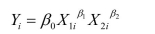
population regression functions below.Write the resulting regression function in a form
that can be estimated by using OLS.
(a)
سؤال
In the case of perfect multicollinearity, OLS is unable to estimate the slope coefficients of the variables involved. Assume that you have included both  as explanatory variables, and that
  , so that there is an exact relationship between two explanatory variables. Does this pose a problem for estimation?
as explanatory variables, and that , so that there is an exact relationship between two explanatory variables. Does this pose a problem for estimation? سؤال
سؤال
سؤال
 (a)Interpret the results.
 سؤال
In the log-log model, the slope coefficient indicates 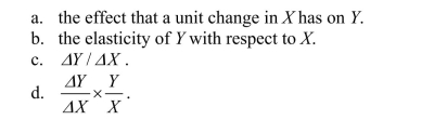
سؤال
There has been much debate about the impact of minimum wages on employment and
unemployment.While most of the focus has been on the employment-to-population ratio
of teenagers, you decide to check if aggregate state unemployment rates have been
affected.Your idea is to see if state unemployment rates for the 48 contiguous U.S.states
in 1985 can predict the unemployment rate for the same states in 1995, and if this
prediction can be improved upon by entering a binary variable for "high impact"
minimum wage states.One labor economist labeled states as high impact if a large
fraction of teenagers was affected by the 1990 and 1991 federal minimum wage
increases.Your first regression results in the following output: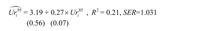 (a)
(a) 
unemployment.While most of the focus has been on the employment-to-population ratio
of teenagers, you decide to check if aggregate state unemployment rates have been
affected.Your idea is to see if state unemployment rates for the 48 contiguous U.S.states
in 1985 can predict the unemployment rate for the same states in 1995, and if this
prediction can be improved upon by entering a binary variable for "high impact"
minimum wage states.One labor economist labeled states as high impact if a large
fraction of teenagers was affected by the 1990 and 1991 federal minimum wage
increases.Your first regression results in the following output:
(a) سؤال
Labor economists have extensively researched the determinants of earnings.Investment
in human capital, measured in years of education, and on the job training are some of the
most important explanatory variables in this research.You decide to apply earnings
functions to the field of sports economics by finding the determinants for baseball pitcher
salaries.You collect data on 455 pitchers for the 1998 baseball season and estimate the
following equation using OLS and heteroskedasticity-robust standard errors: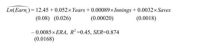 where Earn is annual salary in dollars, Years is number of years in the major leagues,
Innings is number of innings pitched during the career before the 1998 season, Saves is
number of saves during the career before the 1998 season, and ERA is the earned run
average before the 1998 season.
(a)What happens to earnings when the pitcher stays in the league for one additional year?
Compare the salaries of two relievers, one with 10 more saves than the other.What effect
does pitching 100 more innings have on the salary of the pitcher? What effect does
reducing his ERA by 1.5? Do the signs correspond to your expectations? Explain.
in human capital, measured in years of education, and on the job training are some of the
most important explanatory variables in this research.You decide to apply earnings
functions to the field of sports economics by finding the determinants for baseball pitcher
salaries.You collect data on 455 pitchers for the 1998 baseball season and estimate the
following equation using OLS and heteroskedasticity-robust standard errors:
where Earn is annual salary in dollars, Years is number of years in the major leagues,Innings is number of innings pitched during the career before the 1998 season, Saves is
number of saves during the career before the 1998 season, and ERA is the earned run
average before the 1998 season.
(a)What happens to earnings when the pitcher stays in the league for one additional year?
Compare the salaries of two relievers, one with 10 more saves than the other.What effect
does pitching 100 more innings have on the salary of the pitcher? What effect does
reducing his ERA by 1.5? Do the signs correspond to your expectations? Explain.
سؤال
Sports economics typically looks at winning percentages of sports teams as one of
various outputs, and estimates production functions by analyzing the relationship
between the winning percentage and inputs.In Major League Baseball (MLB), the
determinants of winning are quality pitching and batting.All 30 MLB teams for the 1999
season.Pitching quality is approximated by "Team Earned Run Average" (ERA), and
hitting quality by "On Base Plus Slugging Percentage" (OPS).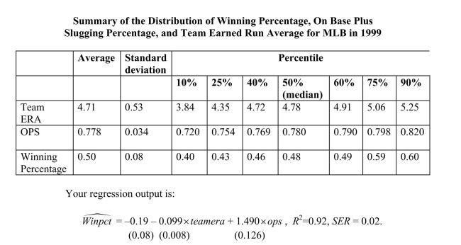 (a)Interpret the regression.Are the results statistically significant and important?
various outputs, and estimates production functions by analyzing the relationship
between the winning percentage and inputs.In Major League Baseball (MLB), the
determinants of winning are quality pitching and batting.All 30 MLB teams for the 1999
season.Pitching quality is approximated by "Team Earned Run Average" (ERA), and
hitting quality by "On Base Plus Slugging Percentage" (OPS).
(a)Interpret the regression.Are the results statistically significant and important? سؤال
سؤال
After analyzing the age-earnings profile for 1,744 workers as shown in the figure, it
becomes clear to you that the relationship cannot be approximately linear.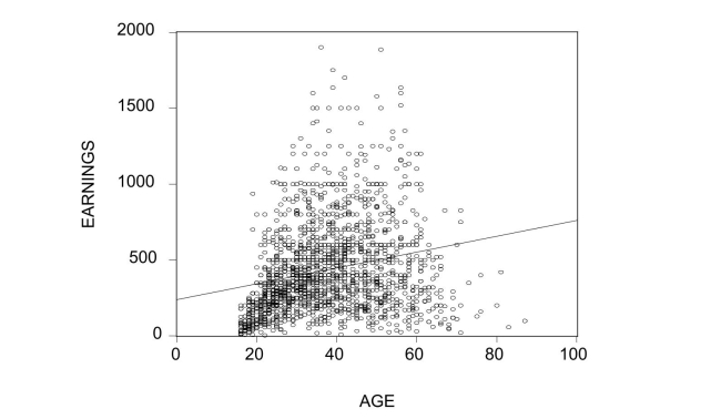 You estimate the following polynomial regression model, controlling for the effect of
gender by using a binary variable that takes on the value of one for females and is zero
otherwise: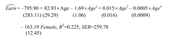 (a)
(a) 
becomes clear to you that the relationship cannot be approximately linear.
You estimate the following polynomial regression model, controlling for the effect ofgender by using a binary variable that takes on the value of one for females and is zero
otherwise:
(a) سؤال
سؤال
Earnings functions attempt to find the determinants of earnings, using both continuous
and binary variables.One of the central questions analyzed in this relationship is the
returns to education.
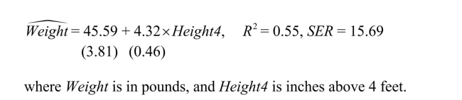
(a)Collecting data from 253 individuals, you estimate the following relationship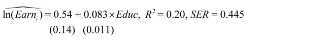 where Earn is average hourly earnings and Educ is years of education.
What is the effect of an additional year of schooling? If you had a strong belief that years
of high school education were different from college education, how would you modify
the equation? What if your theory suggested that there was a "diploma effect"?
and binary variables.One of the central questions analyzed in this relationship is the
returns to education.
(a)Collecting data from 253 individuals, you estimate the following relationship
where Earn is average hourly earnings and Educ is years of education.What is the effect of an additional year of schooling? If you had a strong belief that years
of high school education were different from college education, how would you modify
the equation? What if your theory suggested that there was a "diploma effect"?
سؤال
The figure shows is a plot and a fitted linear regression line of the age-earnings profile of
1,744 individuals, taken from the Current Population Survey.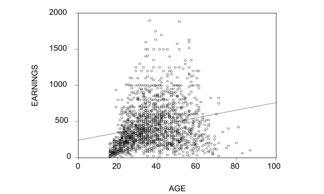 (a)Describe the problems in predicting earnings using the fitted line.What would the pattern
of the residuals look like for the age category under 40?
1,744 individuals, taken from the Current Population Survey.
(a)Describe the problems in predicting earnings using the fitted line.What would the patternof the residuals look like for the age category under 40?
سؤال
Indicate whether or not you can linearize the regression functions below so that OLS
estimation methods can be applied:
(a)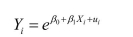
estimation methods can be applied:
(a)
سؤال
An extension of the Solow growth model that includes human capital in addition to
physical capital, suggests that investment in human capital (education)will increase the
wealth of a nation (per capita income).To test this hypothesis, you collect data for 104
countries and perform the following regression: where RelPersInc is GDP per worker relative to the United States, gpop is the average
population growth rate, 1980 to1990, sK is the average investment share of GDP from
1960 to1990, and Educ is the average educational attainment in years for 1985.Numbers
in parentheses are for heteroskedasticity-robust standard errors.
(a)Interpret the results and indicate whether or not the coefficients are significantly different
from zero.Do the coefficients have the expected sign?
physical capital, suggests that investment in human capital (education)will increase the
wealth of a nation (per capita income).To test this hypothesis, you collect data for 104
countries and perform the following regression:
where RelPersInc is GDP per worker relative to the United States, gpop is the averagepopulation growth rate, 1980 to1990, sK is the average investment share of GDP from
1960 to1990, and Educ is the average educational attainment in years for 1985.Numbers
in parentheses are for heteroskedasticity-robust standard errors.
(a)Interpret the results and indicate whether or not the coefficients are significantly different
from zero.Do the coefficients have the expected sign?
سؤال
One of the most frequently estimated equations in the macroeconomics growth literature
are so-called convergence regressions.In essence the average per capita income growth
rate is regressed on the beginning-of-period per capita income level to see if countries
that were further behind initially, grew faster.Some macroeconomic models make this
prediction, once other variables are controlled for.To investigate this matter, you collect
data from 104 countries for the sample period 1960-1990 and estimate the following
relationship (numbers in parentheses are for heteroskedasticity-robust standard errors): where g6090 is the growth rate of GDP per worker for the 1960-1990 sample period,
RelProd60 is the initial starting level of GDP per worker relative to the United States in
1960, gpop is the average population growth rate of the country, and Educ is educational
attainment in years for 1985.
(a)What is the effect of an increase of 5 years in educational attainment? What would
happen if a country could implement policies to cut population growth by one percent?
Are all coefficients significant at the 5% level? If one of the coefficients is not
significant, should you automatically eliminate its variable from the list of explanatory
variables?
are so-called convergence regressions.In essence the average per capita income growth
rate is regressed on the beginning-of-period per capita income level to see if countries
that were further behind initially, grew faster.Some macroeconomic models make this
prediction, once other variables are controlled for.To investigate this matter, you collect
data from 104 countries for the sample period 1960-1990 and estimate the following
relationship (numbers in parentheses are for heteroskedasticity-robust standard errors):
where g6090 is the growth rate of GDP per worker for the 1960-1990 sample period,RelProd60 is the initial starting level of GDP per worker relative to the United States in
1960, gpop is the average population growth rate of the country, and Educ is educational
attainment in years for 1985.
(a)What is the effect of an increase of 5 years in educational attainment? What would
happen if a country could implement policies to cut population growth by one percent?
Are all coefficients significant at the 5% level? If one of the coefficients is not
significant, should you automatically eliminate its variable from the list of explanatory
variables?
سؤال
Earnings functions attempt to predict the log of earnings from a set of explanatory
variables, both binary and continuous.You have allowed for an interaction between two
continuous variables: education and tenure with the current employer.Your estimated
equation is of the following type: where Femme is a binary variable taking on the value of one for females and is zero
otherwise, Educ is the number of years of education, and tenure is continuous years of
work with the current employer.What is the effect of an additional year of education on
earnings ("returns to education")for men? For women? If you allowed for the returns to
education to differ for males and females, how would you respecify the above equation?
What is the effect of an additional year of tenure with a current employer on earnings?
variables, both binary and continuous.You have allowed for an interaction between two
continuous variables: education and tenure with the current employer.Your estimated
equation is of the following type:
where Femme is a binary variable taking on the value of one for females and is zerootherwise, Educ is the number of years of education, and tenure is continuous years of
work with the current employer.What is the effect of an additional year of education on
earnings ("returns to education")for men? For women? If you allowed for the returns to
education to differ for males and females, how would you respecify the above equation?
What is the effect of an additional year of tenure with a current employer on earnings?
سؤال
سؤال
سؤال
Sketch for the log-log model what the relationship between Y and X looks like for various parameter values of the slope, i.e.,
سؤال
Many countries that experience hyperinflation do not have market-determined interest
rates.As a result, some authors have substituted future inflation rates into money demand
equations of the following type as a proxy: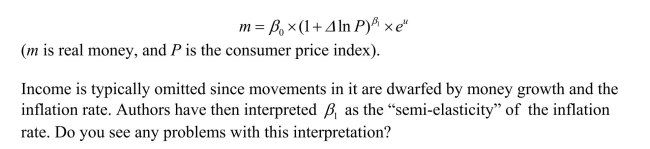
rates.As a result, some authors have substituted future inflation rates into money demand
equations of the following type as a proxy:
سؤال
The textbook shows that 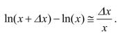 Show that this is equivalent to the following approximation
  if y is small. You use this idea to estimate a demand for money function, which is of the form
 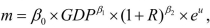 where m is the quantity of (real) money, G D P is the value of (real) Gross Domestic Product, and R is the nominal interest rate. You collect the quarterly data from the Federal Reserve Bank of St. Louis data bank ("FRED"), which lists the money supply and GDP in billions of dollars, prices as an index, and nominal interest rates in percentage points per year You generate the variables in your regression program as follows: m= (money supply)/price index; GDP = (Gross Domestic Product/Price Index), and R= nominal interest rate in percentage points per annum. Next you perform the log-transformations on the real money supply, real G D P , and on (1+R) . Can you for see a problem in using this transformation?
Show that this is equivalent to the following approximation if y is small. You use this idea to estimate a demand for money function, which is of the form where m is the quantity of (real) money, G D P is the value of (real) Gross Domestic Product, and R is the nominal interest rate. You collect the quarterly data from the Federal Reserve Bank of St. Louis data bank ("FRED"), which lists the money supply and GDP in billions of dollars, prices as an index, and nominal interest rates in percentage points per year You generate the variables in your regression program as follows: m= (money supply)/price index; GDP = (Gross Domestic Product/Price Index), and R= nominal interest rate in percentage points per annum. Next you perform the log-transformations on the real money supply, real G D P , and on (1+R) . Can you for see a problem in using this transformation? سؤال
Show that for the following regression model 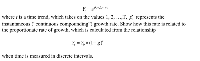
سؤال
سؤال
You have been told that the money demand function in the United States has been unstable since the late 1970 . To investigate this problem, you collect data on the real money supply ( m=M / P ; where M is  and P is the GDP deflator), (real) gross domestic product (G D P) and the nominal interest rate (R) . Next you consider estimating the demand for money using the following alternative functional forms:
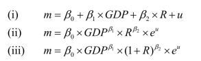
Give an interpretation for in each case. How would you calculate the income elasticity in case (i)?
and P is the GDP deflator), (real) gross domestic product (G D P) and the nominal interest rate (R) . Next you consider estimating the demand for money using the following alternative functional forms:Give an interpretation for
in each case. How would you calculate the income elasticity in case (i)? سؤال
In estimating the original relationship between money wage growth and the unemployment rate, Phillips used United Kingdom data from 1861 to 1913 to fit a curve of the following functional form
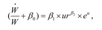
where is the percentage change in money wages and u r is the unemployment rate.
Sketch the function. What role does play? Can you find a linear transformation that allows you to estimate the above function using OLS? If, after taking logarithms on both sides of the equation, you tried to estimate
  using OLS by choosing different values for
  by "trial and error procedure" (Phillips's words), what sort of problem might you run into with the left-hand side variable for some of the observations?
where
is the percentage change in money wages and u r is the unemployment rate.Sketch the function. What role does
play? Can you find a linear transformation that allows you to estimate the above function using OLS? If, after taking logarithms on both sides of the equation, you tried to estimate using OLS by choosing different values for by "trial and error procedure" (Phillips's words), what sort of problem might you run into with the left-hand side variable for some of the observations? سؤال
You have collected data for a cross-section of countries in two time periods, 1960 and 1997, say. Your task is to find the determinants for the Wealth of a Nation (per capita income) and you believe that there are three major determinants: investment in physical capital in both time periods  investment in human capital or education
  and per capita income in the initial period
  You run the following regression:
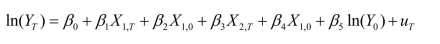
One of your peers suggests that instead, you should run the growth rate in per capita income over the two periods on the change in physical and human capital. For those results to be a parsimonious presentation of your initial regression, what three restrictions would have to hold? How would you test for these? The same person also points out to you that the intercept vanishes in equations where the data is differenced. Is that correct?
investment in human capital or education and per capita income in the initial period You run the following regression:One of your peers suggests that instead, you should run the growth rate in per capita income over the two periods on the change in physical and human capital. For those results to be a parsimonious presentation of your initial regression, what three restrictions would have to hold? How would you test for these? The same person also points out to you that the intercept vanishes in equations where the data is differenced. Is that correct?
سؤال
Being a competitive female swimmer, you wonder if women will ever be able to beat the
time of the male gold medal winner.To investigate this question, you collect data for the
Olympic Games since 1910.At first you consider including various distances, a binary
variable for Mark Spitz, and another binary variable for the arrival and presence of East
German female swimmers, but in the end decide on a simple linear regression.Your
dependent variable is the ratio of the fastest women's time to the fastest men's time in the
100 m backstroke, and the explanatory variable is the year of the Olympics.The
regression result is as follows,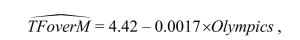 where TFoverM is the relative time of the gold medal winner, and Olympics is the year of
the Olympic Games.What is your prediction when females will catch up to men in this
discipline? Does this sound plausible? What other functional form might you want to
consider?
time of the male gold medal winner.To investigate this question, you collect data for the
Olympic Games since 1910.At first you consider including various distances, a binary
variable for Mark Spitz, and another binary variable for the arrival and presence of East
German female swimmers, but in the end decide on a simple linear regression.Your
dependent variable is the ratio of the fastest women's time to the fastest men's time in the
100 m backstroke, and the explanatory variable is the year of the Olympics.The
regression result is as follows,
where TFoverM is the relative time of the gold medal winner, and Olympics is the year ofthe Olympic Games.What is your prediction when females will catch up to men in this
discipline? Does this sound plausible? What other functional form might you want to
consider?
سؤال

فتح الحزمة
قم بالتسجيل لفتح البطاقات في هذه المجموعة!
Unlock Deck
Unlock Deck
1/53
العب
ملء الشاشة (f)
Deck 8: Nonlinear Regression Functions
1
An example of a quadratic regression model is
C
2
The interpretation of the slope coefficient in the model
is as follows:
A) a 1 % change in X is associated with a change in Y .
B) a 1 % change in X is associated with a change in Y of 0.01
C) a change in X by one unit is associated with a 100 change in Y .
D) a change in X by one unit is associated with a change in Y .
is as follows:
A) a 1 % change in X is associated with a change in Y .
B) a 1 % change in X is associated with a change in Y of 0.01
C) a change in X by one unit is associated with a 100 change in Y .
D) a change in X by one unit is associated with a change in Y .
a 1 % change in X is associated with a change in Y of 0.01
3
To decide whether
fits the data better, you cannot consult the regression R2 because
A) ln (Y) may be negative for 0B) the TSS are not measured in the same units between the two models.
C) the slope no longer indicates the effect of a unit change of X on Y in the log-linear model.
D) the regression can be greater than one in the second model.
fits the data better, you cannot consult the regression R2 because
A) ln (Y) may be negative for 0
C) the slope no longer indicates the effect of a unit change of X on Y in the log-linear model.
D) the regression
can be greater than one in the second model.the TSS are not measured in the same units between the two models.
4
The following interactions between binary and continuous variables are possible, with the exception of
فتح الحزمة
افتح القفل للوصول البطاقات البالغ عددها 53 في هذه المجموعة.
فتح الحزمة
k this deck
5
A polynomial regression model is specified as:
فتح الحزمة
افتح القفل للوصول البطاقات البالغ عددها 53 في هذه المجموعة.
فتح الحزمة
k this deck
6
The best way to interpret polynomial regressions is to
A)take a derivative of Y with respect to the relevant X.
B)plot the estimated regression function and to calculate the estimated effect on Y associated with a change in X for one or more values of X.
C)look at the t-statistics for the relevant coefficients.
D)analyze the standard error of estimated effect.
فتح الحزمة
افتح القفل للوصول البطاقات البالغ عددها 53 في هذه المجموعة.
فتح الحزمة
k this deck
7
In nonlinear models, the expected change in the dependent variable for a change in one of the explanatory variables is given by
فتح الحزمة
افتح القفل للوصول البطاقات البالغ عددها 53 في هذه المجموعة.
فتح الحزمة
k this deck
8
A nonlinear function
A)makes little sense, because variables in the real world are related linearly.
B)can be adequately described by a straight line between the dependent variable and one of the explanatory variables.
C)is a concept that only applies to the case of a single or two explanatory variables since you cannot draw a line in four dimensions.
D)is a function with a slope that is not constant.
فتح الحزمة
افتح القفل للوصول البطاقات البالغ عددها 53 في هذه المجموعة.
فتح الحزمة
k this deck
9
To test whether or not the population regression function is linear rather than a polynomial of order r,
فتح الحزمة
افتح القفل للوصول البطاقات البالغ عددها 53 في هذه المجموعة.
فتح الحزمة
k this deck
10
In the regression model where X is a continuous variable and D is a binary variable,
A) indicates the slope of the regression when D=1 .
B) has a standard error that is not normally distributed even in large samples since D is not a normally distributed variable.
C) indicates the difference in the slopes of the two regressions.
D) has no meaning since
A) indicates the slope of the regression when D=1 .
B) has a standard error that is not normally distributed even in large samples since D is not a normally distributed variable.
C) indicates the difference in the slopes of the two regressions.
D) has no meaning since
فتح الحزمة
افتح القفل للوصول البطاقات البالغ عددها 53 في هذه المجموعة.
فتح الحزمة
k this deck
11
The binary variable interaction regression
A)can only be applied when there are two binary variables, but not three or more.
B)is the same as testing for differences in means.
C)cannot be used with logarithmic regression functions because ln(0)is not defined.
D)allows the effect of changing one of the binary independent variables to depend on the value of the other binary variable.
فتح الحزمة
افتح القفل للوصول البطاقات البالغ عددها 53 في هذه المجموعة.
فتح الحزمة
k this deck
12
The interpretation of the slope coefficient in the model
is as follows:
A) a 1 % change in X is associated with a change in Y .
B) a change in X by one unit is associated with a 100 change in Y .
C) a 1 % change in X is associated with a change in Y of 0.01
D) a change in X by one unit is associated with a change in Y .
is as follows:
A) a 1 % change in X is associated with a change in Y .
B) a change in X by one unit is associated with a 100 change in Y .
C) a 1 % change in X is associated with a change in Y of 0.01
D) a change in X by one unit is associated with a change in Y .
فتح الحزمة
افتح القفل للوصول البطاقات البالغ عددها 53 في هذه المجموعة.
فتح الحزمة
k this deck
13
An example of the interaction term between two independent, continuous variables is
فتح الحزمة
افتح القفل للوصول البطاقات البالغ عددها 53 في هذه المجموعة.
فتح الحزمة
k this deck
14
The following are properties of the logarithm function with the exception of
فتح الحزمة
افتح القفل للوصول البطاقات البالغ عددها 53 في هذه المجموعة.
فتح الحزمة
k this deck
15
You have estimated the following equation:
فتح الحزمة
افتح القفل للوصول البطاقات البالغ عددها 53 في هذه المجموعة.
فتح الحزمة
k this deck
16
(Requires Calculus) In the equation
the following income level results in the maximum test score
A) 607.3 .
B) 91.02 .
C) 45.50 .
D) cannot be determined without a plot of the data.
the following income level results in the maximum test score
A) 607.3 .
B) 91.02 .
C) 45.50 .
D) cannot be determined without a plot of the data.
فتح الحزمة
افتح القفل للوصول البطاقات البالغ عددها 53 في هذه المجموعة.
فتح الحزمة
k this deck
17
The exponential function
فتح الحزمة
افتح القفل للوصول البطاقات البالغ عددها 53 في هذه المجموعة.
فتح الحزمة
k this deck
18
The interpretation of the slope coefficient in the model
is as follows:
A) a 1 % change in X is associated with a change in Y .
B) a change in X by one unit is associated with a change in Y .
C) a change in X by one unit is associated with a 100 change in Y .
D) a 1 % change in X is associated with a change in Y of 0.01
is as follows:
A) a 1 % change in X is associated with a change in Y .
B) a change in X by one unit is associated with a change in Y .
C) a change in X by one unit is associated with a 100 change in Y .
D) a 1 % change in X is associated with a change in Y of 0.01
فتح الحزمة
افتح القفل للوصول البطاقات البالغ عددها 53 في هذه المجموعة.
فتح الحزمة
k this deck
19
For the polynomial regression model,
فتح الحزمة
افتح القفل للوصول البطاقات البالغ عددها 53 في هذه المجموعة.
فتح الحزمة
k this deck
20
Including an interaction term between two independent variables, allows for the following, except that:
A) the interaction term lets the effect on Y of a change in depend on the value of
B) the interaction term coefficient is the effect of a unit increase in and above and beyond the sum of the individual effects of a unit increase in the two variables alone.
C) the interaction term coefficient is the effect of a unit increase in
D) the interaction term lets the effect on Y of a change in depend on the value of
فتح الحزمة
افتح القفل للوصول البطاقات البالغ عددها 53 في هذه المجموعة.
فتح الحزمة
k this deck
21
In the regression model
where X is a continuous
variable and D is a binary variable, to test that the two regressions are identical, you must use the
A) t -statistic separately for
B) F -statistic for the joint hypothesis that
C) t -statistic separately for
D) F -statistic for the joint hypothesis that
where X is a continuous
variable and D is a binary variable, to test that the two regressions are identical, you must use the
A) t -statistic separately for
B) F -statistic for the joint hypothesis that
C) t -statistic separately for
D) F -statistic for the joint hypothesis that
فتح الحزمة
افتح القفل للوصول البطاقات البالغ عددها 53 في هذه المجموعة.
فتح الحزمة
k this deck
22
Give at least three examples from economics where you expect some nonlinearity in the
relationship between variables.Interpret the slope in each case.
relationship between variables.Interpret the slope in each case.
فتح الحزمة
افتح القفل للوصول البطاقات البالغ عددها 53 في هذه المجموعة.
فتح الحزمة
k this deck
23
Choose at least three different nonlinear functional forms of a single independent
variable and sketch the relationship between the dependent and independent variable.
variable and sketch the relationship between the dependent and independent variable.
فتح الحزمة
افتح القفل للوصول البطاقات البالغ عددها 53 في هذه المجموعة.
فتح الحزمة
k this deck
24
Suggest a transformation in the variables that will linearize the deterministic part of the
population regression functions below.Write the resulting regression function in a form
that can be estimated by using OLS.
(a)
population regression functions below.Write the resulting regression function in a form
that can be estimated by using OLS.
(a)
فتح الحزمة
افتح القفل للوصول البطاقات البالغ عددها 53 في هذه المجموعة.
فتح الحزمة
k this deck
25
In the case of perfect multicollinearity, OLS is unable to estimate the slope coefficients of the variables involved. Assume that you have included both as explanatory variables, and that , so that there is an exact relationship between two explanatory variables. Does this pose a problem for estimation?
as explanatory variables, and that , so that there is an exact relationship between two explanatory variables. Does this pose a problem for estimation? فتح الحزمة
افتح القفل للوصول البطاقات البالغ عددها 53 في هذه المجموعة.
فتح الحزمة
k this deck
26
In the model the expected effect is
A)
B)
C)
D)
A)
B)
C)
D)
فتح الحزمة
افتح القفل للوصول البطاقات البالغ عددها 53 في هذه المجموعة.
فتح الحزمة
k this deck
27
You have learned that earnings functions are one of the most investigated relationships in
economics.These typically relate the logarithm of earnings to a series of explanatory
variables such as education, work experience, gender, race, etc.
(a)Why do you think that researchers have preferred a log-linear specification over a linear
specification? In addition to the interpretation of the slope coefficients, also think about
the distribution of the error term.
فتح الحزمة
افتح القفل للوصول البطاقات البالغ عددها 53 في هذه المجموعة.
فتح الحزمة
k this deck
28
(a)Interpret the results. فتح الحزمة
افتح القفل للوصول البطاقات البالغ عددها 53 في هذه المجموعة.
فتح الحزمة
k this deck
29
In the log-log model, the slope coefficient indicates
فتح الحزمة
افتح القفل للوصول البطاقات البالغ عددها 53 في هذه المجموعة.
فتح الحزمة
k this deck
30
There has been much debate about the impact of minimum wages on employment and
unemployment.While most of the focus has been on the employment-to-population ratio
of teenagers, you decide to check if aggregate state unemployment rates have been
affected.Your idea is to see if state unemployment rates for the 48 contiguous U.S.states
in 1985 can predict the unemployment rate for the same states in 1995, and if this
prediction can be improved upon by entering a binary variable for "high impact"
minimum wage states.One labor economist labeled states as high impact if a large
fraction of teenagers was affected by the 1990 and 1991 federal minimum wage
increases.Your first regression results in the following output: (a)
unemployment.While most of the focus has been on the employment-to-population ratio
of teenagers, you decide to check if aggregate state unemployment rates have been
affected.Your idea is to see if state unemployment rates for the 48 contiguous U.S.states
in 1985 can predict the unemployment rate for the same states in 1995, and if this
prediction can be improved upon by entering a binary variable for "high impact"
minimum wage states.One labor economist labeled states as high impact if a large
fraction of teenagers was affected by the 1990 and 1991 federal minimum wage
increases.Your first regression results in the following output:
(a) فتح الحزمة
افتح القفل للوصول البطاقات البالغ عددها 53 في هذه المجموعة.
فتح الحزمة
k this deck
31
Labor economists have extensively researched the determinants of earnings.Investment
in human capital, measured in years of education, and on the job training are some of the
most important explanatory variables in this research.You decide to apply earnings
functions to the field of sports economics by finding the determinants for baseball pitcher
salaries.You collect data on 455 pitchers for the 1998 baseball season and estimate the
following equation using OLS and heteroskedasticity-robust standard errors: where Earn is annual salary in dollars, Years is number of years in the major leagues,
Innings is number of innings pitched during the career before the 1998 season, Saves is
number of saves during the career before the 1998 season, and ERA is the earned run
average before the 1998 season.
(a)What happens to earnings when the pitcher stays in the league for one additional year?
Compare the salaries of two relievers, one with 10 more saves than the other.What effect
does pitching 100 more innings have on the salary of the pitcher? What effect does
reducing his ERA by 1.5? Do the signs correspond to your expectations? Explain.
in human capital, measured in years of education, and on the job training are some of the
most important explanatory variables in this research.You decide to apply earnings
functions to the field of sports economics by finding the determinants for baseball pitcher
salaries.You collect data on 455 pitchers for the 1998 baseball season and estimate the
following equation using OLS and heteroskedasticity-robust standard errors:
where Earn is annual salary in dollars, Years is number of years in the major leagues,Innings is number of innings pitched during the career before the 1998 season, Saves is
number of saves during the career before the 1998 season, and ERA is the earned run
average before the 1998 season.
(a)What happens to earnings when the pitcher stays in the league for one additional year?
Compare the salaries of two relievers, one with 10 more saves than the other.What effect
does pitching 100 more innings have on the salary of the pitcher? What effect does
reducing his ERA by 1.5? Do the signs correspond to your expectations? Explain.
فتح الحزمة
افتح القفل للوصول البطاقات البالغ عددها 53 في هذه المجموعة.
فتح الحزمة
k this deck
32
Sports economics typically looks at winning percentages of sports teams as one of
various outputs, and estimates production functions by analyzing the relationship
between the winning percentage and inputs.In Major League Baseball (MLB), the
determinants of winning are quality pitching and batting.All 30 MLB teams for the 1999
season.Pitching quality is approximated by "Team Earned Run Average" (ERA), and
hitting quality by "On Base Plus Slugging Percentage" (OPS). (a)Interpret the regression.Are the results statistically significant and important?
various outputs, and estimates production functions by analyzing the relationship
between the winning percentage and inputs.In Major League Baseball (MLB), the
determinants of winning are quality pitching and batting.All 30 MLB teams for the 1999
season.Pitching quality is approximated by "Team Earned Run Average" (ERA), and
hitting quality by "On Base Plus Slugging Percentage" (OPS).
(a)Interpret the regression.Are the results statistically significant and important? فتح الحزمة
افتح القفل للوصول البطاقات البالغ عددها 53 في هذه المجموعة.
فتح الحزمة
k this deck
33
Females, it is said, make 70 cents to the dollar in the United States.To investigate this
phenomenon, you collect data on weekly earnings from 1,744 individuals, 850 females
and 894 males.Next, you calculate their average weekly earnings and find that the
females in your sample earned $346.98, while the males made $517.70.
(a)Calculate the female earnings in percent of the male earnings.How would you test
whether or not this difference is statistically significant? Give two approaches.
فتح الحزمة
افتح القفل للوصول البطاقات البالغ عددها 53 في هذه المجموعة.
فتح الحزمة
k this deck
34
After analyzing the age-earnings profile for 1,744 workers as shown in the figure, it
becomes clear to you that the relationship cannot be approximately linear. You estimate the following polynomial regression model, controlling for the effect of
gender by using a binary variable that takes on the value of one for females and is zero
otherwise: (a)
becomes clear to you that the relationship cannot be approximately linear.
You estimate the following polynomial regression model, controlling for the effect ofgender by using a binary variable that takes on the value of one for females and is zero
otherwise:
(a) فتح الحزمة
افتح القفل للوصول البطاقات البالغ عددها 53 في هذه المجموعة.
فتح الحزمة
k this deck
35
In the regression model where X is a continuous variable and D is a binary variable,
A) is the difference in means in Y between the two categories.
B) indicates the difference in the intercepts of the two regressions.
C) is usually positive.
D) indicates the difference in the slopes of the two regressions.
A) is the difference in means in Y between the two categories.
B) indicates the difference in the intercepts of the two regressions.
C) is usually positive.
D) indicates the difference in the slopes of the two regressions.
فتح الحزمة
افتح القفل للوصول البطاقات البالغ عددها 53 في هذه المجموعة.
فتح الحزمة
k this deck
36
Earnings functions attempt to find the determinants of earnings, using both continuous
and binary variables.One of the central questions analyzed in this relationship is the
returns to education.
(a)Collecting data from 253 individuals, you estimate the following relationship where Earn is average hourly earnings and Educ is years of education.
What is the effect of an additional year of schooling? If you had a strong belief that years
of high school education were different from college education, how would you modify
the equation? What if your theory suggested that there was a "diploma effect"?
and binary variables.One of the central questions analyzed in this relationship is the
returns to education.
(a)Collecting data from 253 individuals, you estimate the following relationship
where Earn is average hourly earnings and Educ is years of education.What is the effect of an additional year of schooling? If you had a strong belief that years
of high school education were different from college education, how would you modify
the equation? What if your theory suggested that there was a "diploma effect"?
فتح الحزمة
افتح القفل للوصول البطاقات البالغ عددها 53 في هذه المجموعة.
فتح الحزمة
k this deck
37
The figure shows is a plot and a fitted linear regression line of the age-earnings profile of
1,744 individuals, taken from the Current Population Survey. (a)Describe the problems in predicting earnings using the fitted line.What would the pattern
of the residuals look like for the age category under 40?
1,744 individuals, taken from the Current Population Survey.
(a)Describe the problems in predicting earnings using the fitted line.What would the patternof the residuals look like for the age category under 40?
فتح الحزمة
افتح القفل للوصول البطاقات البالغ عددها 53 في هذه المجموعة.
فتح الحزمة
k this deck
38
Indicate whether or not you can linearize the regression functions below so that OLS
estimation methods can be applied:
(a)
estimation methods can be applied:
(a)
فتح الحزمة
افتح القفل للوصول البطاقات البالغ عددها 53 في هذه المجموعة.
فتح الحزمة
k this deck
39
An extension of the Solow growth model that includes human capital in addition to
physical capital, suggests that investment in human capital (education)will increase the
wealth of a nation (per capita income).To test this hypothesis, you collect data for 104
countries and perform the following regression: where RelPersInc is GDP per worker relative to the United States, gpop is the average
population growth rate, 1980 to1990, sK is the average investment share of GDP from
1960 to1990, and Educ is the average educational attainment in years for 1985.Numbers
in parentheses are for heteroskedasticity-robust standard errors.
(a)Interpret the results and indicate whether or not the coefficients are significantly different
from zero.Do the coefficients have the expected sign?
physical capital, suggests that investment in human capital (education)will increase the
wealth of a nation (per capita income).To test this hypothesis, you collect data for 104
countries and perform the following regression:
where RelPersInc is GDP per worker relative to the United States, gpop is the averagepopulation growth rate, 1980 to1990, sK is the average investment share of GDP from
1960 to1990, and Educ is the average educational attainment in years for 1985.Numbers
in parentheses are for heteroskedasticity-robust standard errors.
(a)Interpret the results and indicate whether or not the coefficients are significantly different
from zero.Do the coefficients have the expected sign?
فتح الحزمة
افتح القفل للوصول البطاقات البالغ عددها 53 في هذه المجموعة.
فتح الحزمة
k this deck
40
One of the most frequently estimated equations in the macroeconomics growth literature
are so-called convergence regressions.In essence the average per capita income growth
rate is regressed on the beginning-of-period per capita income level to see if countries
that were further behind initially, grew faster.Some macroeconomic models make this
prediction, once other variables are controlled for.To investigate this matter, you collect
data from 104 countries for the sample period 1960-1990 and estimate the following
relationship (numbers in parentheses are for heteroskedasticity-robust standard errors): where g6090 is the growth rate of GDP per worker for the 1960-1990 sample period,
RelProd60 is the initial starting level of GDP per worker relative to the United States in
1960, gpop is the average population growth rate of the country, and Educ is educational
attainment in years for 1985.
(a)What is the effect of an increase of 5 years in educational attainment? What would
happen if a country could implement policies to cut population growth by one percent?
Are all coefficients significant at the 5% level? If one of the coefficients is not
significant, should you automatically eliminate its variable from the list of explanatory
variables?
are so-called convergence regressions.In essence the average per capita income growth
rate is regressed on the beginning-of-period per capita income level to see if countries
that were further behind initially, grew faster.Some macroeconomic models make this
prediction, once other variables are controlled for.To investigate this matter, you collect
data from 104 countries for the sample period 1960-1990 and estimate the following
relationship (numbers in parentheses are for heteroskedasticity-robust standard errors):
where g6090 is the growth rate of GDP per worker for the 1960-1990 sample period,RelProd60 is the initial starting level of GDP per worker relative to the United States in
1960, gpop is the average population growth rate of the country, and Educ is educational
attainment in years for 1985.
(a)What is the effect of an increase of 5 years in educational attainment? What would
happen if a country could implement policies to cut population growth by one percent?
Are all coefficients significant at the 5% level? If one of the coefficients is not
significant, should you automatically eliminate its variable from the list of explanatory
variables?
فتح الحزمة
افتح القفل للوصول البطاقات البالغ عددها 53 في هذه المجموعة.
فتح الحزمة
k this deck
41
Earnings functions attempt to predict the log of earnings from a set of explanatory
variables, both binary and continuous.You have allowed for an interaction between two
continuous variables: education and tenure with the current employer.Your estimated
equation is of the following type: where Femme is a binary variable taking on the value of one for females and is zero
otherwise, Educ is the number of years of education, and tenure is continuous years of
work with the current employer.What is the effect of an additional year of education on
earnings ("returns to education")for men? For women? If you allowed for the returns to
education to differ for males and females, how would you respecify the above equation?
What is the effect of an additional year of tenure with a current employer on earnings?
variables, both binary and continuous.You have allowed for an interaction between two
continuous variables: education and tenure with the current employer.Your estimated
equation is of the following type:
where Femme is a binary variable taking on the value of one for females and is zerootherwise, Educ is the number of years of education, and tenure is continuous years of
work with the current employer.What is the effect of an additional year of education on
earnings ("returns to education")for men? For women? If you allowed for the returns to
education to differ for males and females, how would you respecify the above equation?
What is the effect of an additional year of tenure with a current employer on earnings?
فتح الحزمة
افتح القفل للوصول البطاقات البالغ عددها 53 في هذه المجموعة.
فتح الحزمة
k this deck
42
To investigate whether or not there is discrimination against a sub-group of individuals,
you regress the log of earnings on determining variables, such as education, work
experience, etc., and a binary variable which takes on the value of one for individuals in
that sub-group and is zero otherwise.You consider two possible specifications.First you
run two separate regressions, one for the observations that include the sub-group and one
for the others.Second, you run a single regression, but allow for a binary variable to
appear in the regression.Your professor suggests that the second equation is better for the
task at hand, as long as you allow for a shift in both the intercept and the slopes.Explain
her reasoning.
فتح الحزمة
افتح القفل للوصول البطاقات البالغ عددها 53 في هذه المجموعة.
فتح الحزمة
k this deck
43
(Requires Calculus)Show that for the log-log model the slope coefficient is the
elasticity.
elasticity.
فتح الحزمة
افتح القفل للوصول البطاقات البالغ عددها 53 في هذه المجموعة.
فتح الحزمة
k this deck
44
Sketch for the log-log model what the relationship between Y and X looks like for various parameter values of the slope, i.e.,
فتح الحزمة
افتح القفل للوصول البطاقات البالغ عددها 53 في هذه المجموعة.
فتح الحزمة
k this deck
45
Many countries that experience hyperinflation do not have market-determined interest
rates.As a result, some authors have substituted future inflation rates into money demand
equations of the following type as a proxy:
rates.As a result, some authors have substituted future inflation rates into money demand
equations of the following type as a proxy:
فتح الحزمة
افتح القفل للوصول البطاقات البالغ عددها 53 في هذه المجموعة.
فتح الحزمة
k this deck
46
The textbook shows that Show that this is equivalent to the following approximation if y is small. You use this idea to estimate a demand for money function, which is of the form where m is the quantity of (real) money, G D P is the value of (real) Gross Domestic Product, and R is the nominal interest rate. You collect the quarterly data from the Federal Reserve Bank of St. Louis data bank ("FRED"), which lists the money supply and GDP in billions of dollars, prices as an index, and nominal interest rates in percentage points per year You generate the variables in your regression program as follows: m= (money supply)/price index; GDP = (Gross Domestic Product/Price Index), and R= nominal interest rate in percentage points per annum. Next you perform the log-transformations on the real money supply, real G D P , and on (1+R) . Can you for see a problem in using this transformation?
Show that this is equivalent to the following approximation if y is small. You use this idea to estimate a demand for money function, which is of the form where m is the quantity of (real) money, G D P is the value of (real) Gross Domestic Product, and R is the nominal interest rate. You collect the quarterly data from the Federal Reserve Bank of St. Louis data bank ("FRED"), which lists the money supply and GDP in billions of dollars, prices as an index, and nominal interest rates in percentage points per year You generate the variables in your regression program as follows: m= (money supply)/price index; GDP = (Gross Domestic Product/Price Index), and R= nominal interest rate in percentage points per annum. Next you perform the log-transformations on the real money supply, real G D P , and on (1+R) . Can you for see a problem in using this transformation? فتح الحزمة
افتح القفل للوصول البطاقات البالغ عددها 53 في هذه المجموعة.
فتح الحزمة
k this deck
47
Show that for the following regression model
فتح الحزمة
افتح القفل للوصول البطاقات البالغ عددها 53 في هذه المجموعة.
فتح الحزمة
k this deck
48
Your task is to estimate the ice cream sales for a certain chain in New England.The
company makes available to you quarterly ice cream sales (Y)and informs you that the
price per gallon has approximately remained constant over the sample period.You gather
information on average daily temperatures (X)during these quarters and regress Y on X,
adding seasonal binary variables for spring, summer, and fall.These variables are
constructed as follows: DSpring takes on a value of 1 during the spring and is zero
otherwise, DSummer takes on a value of 1 during the summer, etc.Specify three
regression functions where the following conditions hold: the relationship between Y and
X is (i)forced to be the same for each quarter; (ii)allowed to have different intercepts
each season; (iii)allowed to have varying slopes and intercepts each season.Sketch the
difference between (i)and (ii).How would you test which model fits the data the best?
فتح الحزمة
افتح القفل للوصول البطاقات البالغ عددها 53 في هذه المجموعة.
فتح الحزمة
k this deck
49
You have been told that the money demand function in the United States has been unstable since the late 1970 . To investigate this problem, you collect data on the real money supply ( m=M / P ; where M is and P is the GDP deflator), (real) gross domestic product (G D P) and the nominal interest rate (R) . Next you consider estimating the demand for money using the following alternative functional forms:
Give an interpretation for in each case. How would you calculate the income elasticity in case (i)?
and P is the GDP deflator), (real) gross domestic product (G D P) and the nominal interest rate (R) . Next you consider estimating the demand for money using the following alternative functional forms:Give an interpretation for
in each case. How would you calculate the income elasticity in case (i)? فتح الحزمة
افتح القفل للوصول البطاقات البالغ عددها 53 في هذه المجموعة.
فتح الحزمة
k this deck
50
In estimating the original relationship between money wage growth and the unemployment rate, Phillips used United Kingdom data from 1861 to 1913 to fit a curve of the following functional form
where is the percentage change in money wages and u r is the unemployment rate.
Sketch the function. What role does play? Can you find a linear transformation that allows you to estimate the above function using OLS? If, after taking logarithms on both sides of the equation, you tried to estimate using OLS by choosing different values for by "trial and error procedure" (Phillips's words), what sort of problem might you run into with the left-hand side variable for some of the observations?
where
is the percentage change in money wages and u r is the unemployment rate.Sketch the function. What role does
play? Can you find a linear transformation that allows you to estimate the above function using OLS? If, after taking logarithms on both sides of the equation, you tried to estimate using OLS by choosing different values for by "trial and error procedure" (Phillips's words), what sort of problem might you run into with the left-hand side variable for some of the observations? فتح الحزمة
افتح القفل للوصول البطاقات البالغ عددها 53 في هذه المجموعة.
فتح الحزمة
k this deck
51
You have collected data for a cross-section of countries in two time periods, 1960 and 1997, say. Your task is to find the determinants for the Wealth of a Nation (per capita income) and you believe that there are three major determinants: investment in physical capital in both time periods investment in human capital or education and per capita income in the initial period You run the following regression:
One of your peers suggests that instead, you should run the growth rate in per capita income over the two periods on the change in physical and human capital. For those results to be a parsimonious presentation of your initial regression, what three restrictions would have to hold? How would you test for these? The same person also points out to you that the intercept vanishes in equations where the data is differenced. Is that correct?
investment in human capital or education and per capita income in the initial period You run the following regression:One of your peers suggests that instead, you should run the growth rate in per capita income over the two periods on the change in physical and human capital. For those results to be a parsimonious presentation of your initial regression, what three restrictions would have to hold? How would you test for these? The same person also points out to you that the intercept vanishes in equations where the data is differenced. Is that correct?
فتح الحزمة
افتح القفل للوصول البطاقات البالغ عددها 53 في هذه المجموعة.
فتح الحزمة
k this deck
52
Being a competitive female swimmer, you wonder if women will ever be able to beat the
time of the male gold medal winner.To investigate this question, you collect data for the
Olympic Games since 1910.At first you consider including various distances, a binary
variable for Mark Spitz, and another binary variable for the arrival and presence of East
German female swimmers, but in the end decide on a simple linear regression.Your
dependent variable is the ratio of the fastest women's time to the fastest men's time in the
100 m backstroke, and the explanatory variable is the year of the Olympics.The
regression result is as follows, where TFoverM is the relative time of the gold medal winner, and Olympics is the year of
the Olympic Games.What is your prediction when females will catch up to men in this
discipline? Does this sound plausible? What other functional form might you want to
consider?
time of the male gold medal winner.To investigate this question, you collect data for the
Olympic Games since 1910.At first you consider including various distances, a binary
variable for Mark Spitz, and another binary variable for the arrival and presence of East
German female swimmers, but in the end decide on a simple linear regression.Your
dependent variable is the ratio of the fastest women's time to the fastest men's time in the
100 m backstroke, and the explanatory variable is the year of the Olympics.The
regression result is as follows,
where TFoverM is the relative time of the gold medal winner, and Olympics is the year ofthe Olympic Games.What is your prediction when females will catch up to men in this
discipline? Does this sound plausible? What other functional form might you want to
consider?
فتح الحزمة
افتح القفل للوصول البطاقات البالغ عددها 53 في هذه المجموعة.
فتح الحزمة
k this deck
53
Assume that you had data for a cross-section of 100 households with data on
consumption and personal disposable income.If you fit a linear regression function
regressing consumption on disposable income, what prior expectations do you have about
the slope and the intercept? The slope of this regression function is called the "marginal
propensity to consume." If, instead, you fit a log-log model, then what is the
interpretation of the slope? Do you have any prior expectation about its size?
فتح الحزمة
افتح القفل للوصول البطاقات البالغ عددها 53 في هذه المجموعة.
فتح الحزمة
k this deck
فتح الحزمة
افتح القفل للوصول البطاقات البالغ عددها 53 في هذه المجموعة.


