Deck 15: Estimation of Dynamic Causal Effects
ملء الشاشة (f)
سؤال
سؤال
سؤال
Quasi differences in Yt are defined as 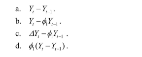
سؤال
سؤال
سؤال
سؤال
The impact effect is the 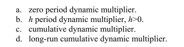
سؤال
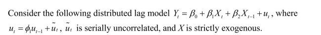
The distributed lag model is given by 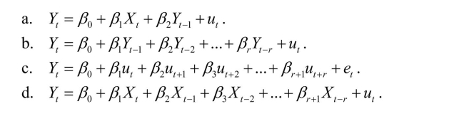
سؤال
The long-run cumulative dynamic multiplier 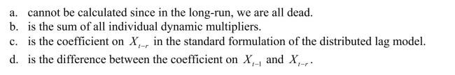
سؤال
سؤال
سؤال
A distributed lag regression 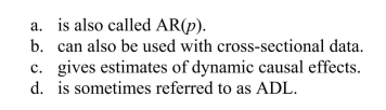
سؤال
سؤال
سؤال
سؤال
Infeasible GLS 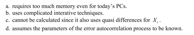
سؤال
سؤال
سؤال
سؤال
سؤال
سؤال
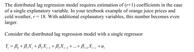
 (a)How many parameters are there to be estimated between the two equations?
 سؤال
سؤال
The Gallup Poll frequently surveys the electorate to quantify the public's opinion of the
president.Since 1945, Gallup settled on the following wording of its presidential poll:
"Do you approve or disapprove of the way (name)is handling his job as president?"
Gallup has not changed its presidential question since then, and respondents can answer
"approve," "disapprove," or "no opinion."
You want to see how this approval rating is related to the Michigan index of consumer
sentiment (ICS).The monthly survey, conducted with a minimum sample of 500, asks
people if they feel "better/worse off" with regard to current and future conditions.
(a)To estimate dynamic causal effects, you collect quarterly data from 1962:I - 1998:II for
the United States.You allow a binary variable for each presidency to capture the intrinsic
popularity of the President.Furthermore, you eliminate observations that include a
change in party for the presidency by using a binary variable, which takes on the value of
one during the first quarter of the year after the election.Finally, a friendly political
scientist provides you with (i)an "events" variable, (ii)a "Vietnam" binary variable, and
(iii)a "honeymoon" variable, which measures the effect of a higher popularity of a
president immediately following the election.(The coefficients of these variables will not
be reported here.)
Assuming that consumer sentiment is exogenous, you estimate the following two
specifications (numbers in parenthesis are heteroskedasticity- and autocorrelation-
consistent standard errors)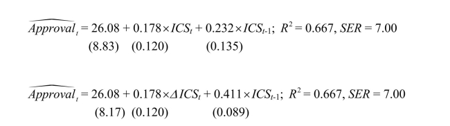 What is the difference between the two specifications? What is the advantage of
estimating the second equation, if any?
president.Since 1945, Gallup settled on the following wording of its presidential poll:
"Do you approve or disapprove of the way (name)is handling his job as president?"
Gallup has not changed its presidential question since then, and respondents can answer
"approve," "disapprove," or "no opinion."
You want to see how this approval rating is related to the Michigan index of consumer
sentiment (ICS).The monthly survey, conducted with a minimum sample of 500, asks
people if they feel "better/worse off" with regard to current and future conditions.
(a)To estimate dynamic causal effects, you collect quarterly data from 1962:I - 1998:II for
the United States.You allow a binary variable for each presidency to capture the intrinsic
popularity of the President.Furthermore, you eliminate observations that include a
change in party for the presidency by using a binary variable, which takes on the value of
one during the first quarter of the year after the election.Finally, a friendly political
scientist provides you with (i)an "events" variable, (ii)a "Vietnam" binary variable, and
(iii)a "honeymoon" variable, which measures the effect of a higher popularity of a
president immediately following the election.(The coefficients of these variables will not
be reported here.)
Assuming that consumer sentiment is exogenous, you estimate the following two
specifications (numbers in parenthesis are heteroskedasticity- and autocorrelation-
consistent standard errors)
What is the difference between the two specifications? What is the advantage ofestimating the second equation, if any?
سؤال
The distributed lag model assumptions include all of the following with the exception of 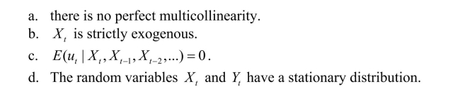
سؤال
 (a)Give an example what the authors have in mind.
 سؤال
In your intermediate macroeconomics course, government expenditures and the money
supply were treated as exogenous, in the sense that the variables could be changed to
conduct economic policy to influence target variables, but that these variables would not
react to changes in the economy as a result of some fixed rule.The St.Louis Model,
proposed by two researchers at the Federal Reserve in St.Louis, used this idea to test
whether monetary policy or fiscal policy was more effective in influencing output
behavior.Although there were various versions of this model, the basic specification was
of the following type: Assuming that money supply and government expenditures are exogenous, how would
you estimate dynamic causal effects? Why do you think this type of model is no longer
used by most to calculate fiscal and monetary multipliers?
supply were treated as exogenous, in the sense that the variables could be changed to
conduct economic policy to influence target variables, but that these variables would not
react to changes in the economy as a result of some fixed rule.The St.Louis Model,
proposed by two researchers at the Federal Reserve in St.Louis, used this idea to test
whether monetary policy or fiscal policy was more effective in influencing output
behavior.Although there were various versions of this model, the basic specification was
of the following type:
Assuming that money supply and government expenditures are exogenous, how wouldyou estimate dynamic causal effects? Why do you think this type of model is no longer
used by most to calculate fiscal and monetary multipliers?
سؤال
 (a)
(a) 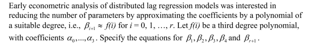
سؤال
Your textbook used a distributed lag model with only current and past values of Xt-1
coupled with an AR(1)error model to derive a quasi-difference model, where the error
term was uncorrelated.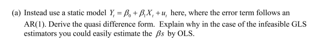
coupled with an AR(1)error model to derive a quasi-difference model, where the error
term was uncorrelated.
سؤال
سؤال
سؤال
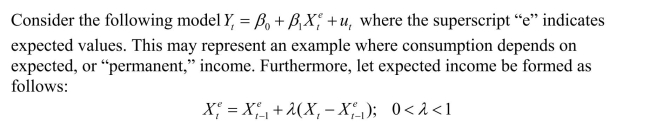 (a)In the above expectation formation hypothesis, expectations are formed at the end of the
period, say the
 of December, if you had annual data.Give an intuitive explanation for
this process.
سؤال
The distributed lag model relating orange juice prices to the Orlando weather reported in
the text was of the form (a)Suppose that an agricultural economist tells you that a freeze in December is more
harmful than a freeze in the other months.How would you modify the regression to
incorporate this effect? How would you test for this December effect?
the text was of the form
(a)Suppose that an agricultural economist tells you that a freeze in December is moreharmful than a freeze in the other months.How would you modify the regression to
incorporate this effect? How would you test for this December effect?
سؤال
سؤال
GLS is consistent and BLUE if 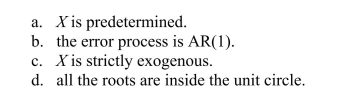
سؤال
سؤال
سؤال
A model that attracted quite a bit of interest in macroeconomics in the 1970s was the St.
Louis model.The underlying idea was to calculate fiscal and monetary impact and long
run cumulative dynamic multipliers, by relating output (growth)to government
expenditure (growth)and money supply (growth).The assumption was that both
government expenditures and the money supply were exogenous.Estimation of a St.
Louis type model using quarterly data from 1960:I-1995:IV results in the following
output (HAC standard errors in parenthesis):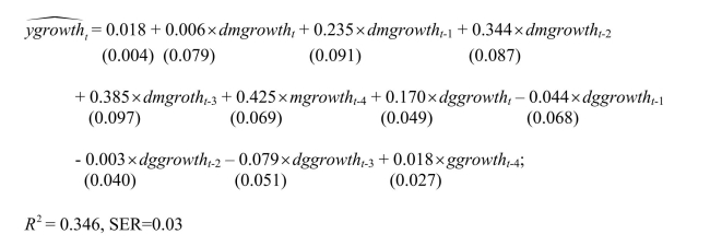 where ygrowth is quarterly growth of real GDP, mgrowth is quarterly growth of real
  (a)Assuming that money and government expenditures are exogenous, what do the
coefficients represent? Calculate the h-period cumulative dynamic multipliers from these.
How can you test for the statistical significance of the cumulative dynamic multipliers
and the long-run cumulative dynamic multiplier?
Louis model.The underlying idea was to calculate fiscal and monetary impact and long
run cumulative dynamic multipliers, by relating output (growth)to government
expenditure (growth)and money supply (growth).The assumption was that both
government expenditures and the money supply were exogenous.Estimation of a St.
Louis type model using quarterly data from 1960:I-1995:IV results in the following
output (HAC standard errors in parenthesis):
where ygrowth is quarterly growth of real GDP, mgrowth is quarterly growth of real (a)Assuming that money and government expenditures are exogenous, what do thecoefficients represent? Calculate the h-period cumulative dynamic multipliers from these.
How can you test for the statistical significance of the cumulative dynamic multipliers
and the long-run cumulative dynamic multiplier?
سؤال
It has been argued that Canada's aggregate output growth and unemployment rates are
very sensitive to United States economic fluctuations, while the opposite is not true.
(a)A researcher uses a distributed lag model to estimate dynamic causal effects of U.S.
economic activity on Canada.The results (HAC standard errors in parenthesis)for the
sample period 1961:I-1995:IV are: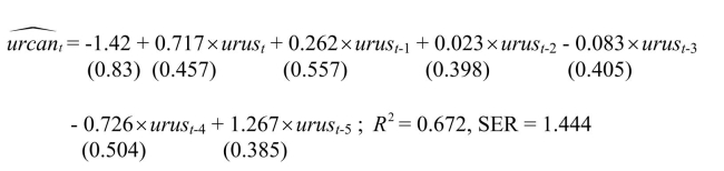 where urcan is the Canadian unemployment rate, and urus is the United States
unemployment rate.
Calculate the long-run cumulative dynamic multiplier.
very sensitive to United States economic fluctuations, while the opposite is not true.
(a)A researcher uses a distributed lag model to estimate dynamic causal effects of U.S.
economic activity on Canada.The results (HAC standard errors in parenthesis)for the
sample period 1961:I-1995:IV are:
where urcan is the Canadian unemployment rate, and urus is the United Statesunemployment rate.
Calculate the long-run cumulative dynamic multiplier.
سؤال
One of the central predictions of neo-classical macroeconomic growth theory is that an
increase in the growth rate of the population causes at first a decline the growth rate of
real output per capita, but that subsequently the growth rate returns to its natural level,
itself determined by the rate of technological innovation.The intuition is that, if the
growth rate of the workforce increases, then more has to be saved to provide the new
workers with physical capital.However, accumulating capital takes time, so that output
per capita falls in the short run.
Under the assumption that population growth is exogenous, a number of regressions of
the growth rate of output per capita on current and lagged population growth were
performed, as reported below.(A constant was included in the regressions but is not
reported.HAC standard errors are in brackets.BIC is listed at the bottom of the table).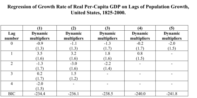 (a)Which of these models is favored by the information criterion?
increase in the growth rate of the population causes at first a decline the growth rate of
real output per capita, but that subsequently the growth rate returns to its natural level,
itself determined by the rate of technological innovation.The intuition is that, if the
growth rate of the workforce increases, then more has to be saved to provide the new
workers with physical capital.However, accumulating capital takes time, so that output
per capita falls in the short run.
Under the assumption that population growth is exogenous, a number of regressions of
the growth rate of output per capita on current and lagged population growth were
performed, as reported below.(A constant was included in the regressions but is not
reported.HAC standard errors are in brackets.BIC is listed at the bottom of the table).
(a)Which of these models is favored by the information criterion?
فتح الحزمة
قم بالتسجيل لفتح البطاقات في هذه المجموعة!
Unlock Deck
Unlock Deck
1/40
العب
ملء الشاشة (f)
Deck 15: Estimation of Dynamic Causal Effects
1
Ascertaining whether or not a regressor is strictly exogenous or exogenous ultimately requires all of the following with the exception of
A)economic theory.
B)institutional knowledge.
C)expert judgment.
D)use of HAC standard errors.
A)economic theory.
B)institutional knowledge.
C)expert judgment.
D)use of HAC standard errors.
D
2
GLS
A)results in smaller variances of the estimator than OLS if the regressors are strictly exogenous.
B)is the same as OLS using HAC standard errors.
C)can be used even if the regressors are not strictly exogenous.
D)can be used for time-series estimation, but not in cross-sectional data.
A)results in smaller variances of the estimator than OLS if the regressors are strictly exogenous.
B)is the same as OLS using HAC standard errors.
C)can be used even if the regressors are not strictly exogenous.
D)can be used for time-series estimation, but not in cross-sectional data.
A
3
Quasi differences in Yt are defined as
B
4
The concept of exogeneity is important because
A)it clarifies whether or not the variable is determined inside or outside your model.
B)maximum likelihood estimation is no longer valid.
C)under strict exogeneity, OLS may not be efficient as an estimator of dynamic causal effects.
D)endogenous variables are not stationary, but exogenous variables are.
فتح الحزمة
افتح القفل للوصول البطاقات البالغ عددها 40 في هذه المجموعة.
فتح الحزمة
k this deck
5
In time series, the definition of causal effects
A)says that one variable helps predict another variable.
B)does not make much sense since there are not multiple subjects.
C)assumes that the same subject is being given different treatments at different points in time.
D)requires panel data.
A)says that one variable helps predict another variable.
B)does not make much sense since there are not multiple subjects.
C)assumes that the same subject is being given different treatments at different points in time.
D)requires panel data.
فتح الحزمة
افتح القفل للوصول البطاقات البالغ عددها 40 في هذه المجموعة.
فتح الحزمة
k this deck
6
Estimation of dynamic multipliers under strict exogeneity should be done by
A)instrumental variable methods.
B)OLS.
C)feasible GLS.
D)analyzing the stationarity of the multipliers.
A)instrumental variable methods.
B)OLS.
C)feasible GLS.
D)analyzing the stationarity of the multipliers.
فتح الحزمة
افتح القفل للوصول البطاقات البالغ عددها 40 في هذه المجموعة.
فتح الحزمة
k this deck
7
The impact effect is the
فتح الحزمة
افتح القفل للوصول البطاقات البالغ عددها 40 في هذه المجموعة.
فتح الحزمة
k this deck
8
The distributed lag model is given by
فتح الحزمة
افتح القفل للوصول البطاقات البالغ عددها 40 في هذه المجموعة.
فتح الحزمة
k this deck
9
The long-run cumulative dynamic multiplier
فتح الحزمة
افتح القفل للوصول البطاقات البالغ عددها 40 في هذه المجموعة.
فتح الحزمة
k this deck
10
GLS involves
A)writing the model in differences and estimating it by OLS, using HAC standard errors.
B)truncating the sample at both ends of the period, then estimating by OLS using HAC standard errors.
C)checking the AIC rather than the BIC in choosing the maximum lag-length of the regressors.
D)transforming the regression model so that the errors are homoskedastic and serially uncorrelated, and then estimating the transformed regression model by
OLS)
فتح الحزمة
افتح القفل للوصول البطاقات البالغ عددها 40 في هذه المجموعة.
فتح الحزمة
k this deck
11
To convey information about the dynamic multipliers more effectively, you should
A)plot them.
B)discuss these carefully one at a time.
C)estimate them by maximum likelihood methods.
D)first make sure that they are stationary.
A)plot them.
B)discuss these carefully one at a time.
C)estimate them by maximum likelihood methods.
D)first make sure that they are stationary.
فتح الحزمة
افتح القفل للوصول البطاقات البالغ عددها 40 في هذه المجموعة.
فتح الحزمة
k this deck
12
A distributed lag regression
فتح الحزمة
افتح القفل للوصول البطاقات البالغ عددها 40 في هذه المجموعة.
فتح الحزمة
k this deck
13
Sensitivity analysis of the results may include the following with the exception of
A)stability over time analysis of the estimated multipliers.
B)using homoskedasticity only rather than HAC standard errors.
C)investigation of omitted variable bias.
D)looking at different computations of the HAC standard errors.
A)stability over time analysis of the estimated multipliers.
B)using homoskedasticity only rather than HAC standard errors.
C)investigation of omitted variable bias.
D)looking at different computations of the HAC standard errors.
فتح الحزمة
افتح القفل للوصول البطاقات البالغ عددها 40 في هذه المجموعة.
فتح الحزمة
k this deck
14
The 95% confidence interval for the dynamic multipliers should be computed by using the estimated coefficient
A) 1.96 times the RMSFE.
B) 1.96 times the HAC standard errors.
C) 1.96 , since the HAC errors are standardized.
D) 1.64 times the HAC standard errors since the alternative hypothesis is one-sided.
A) 1.96 times the RMSFE.
B) 1.96 times the HAC standard errors.
C) 1.96 , since the HAC errors are standardized.
D) 1.64 times the HAC standard errors since the alternative hypothesis is one-sided.
فتح الحزمة
افتح القفل للوصول البطاقات البالغ عددها 40 في هذه المجموعة.
فتح الحزمة
k this deck
15
The concepts of exogeneity, strict exogeneity, and predeterminedness
A)are defined in such a way that strict exogeneity implies exogeneity.
B)Can be used interchangeably.
C)Are defined in such a way that exogeneity implies strict exogeneity.
D)Correspond to endogeneity, strict endogeneity, and lagged endogenous variables.
A)are defined in such a way that strict exogeneity implies exogeneity.
B)Can be used interchangeably.
C)Are defined in such a way that exogeneity implies strict exogeneity.
D)Correspond to endogeneity, strict endogeneity, and lagged endogenous variables.
فتح الحزمة
افتح القفل للوصول البطاقات البالغ عددها 40 في هذه المجموعة.
فتح الحزمة
k this deck
16
Infeasible GLS
فتح الحزمة
افتح القفل للوصول البطاقات البالغ عددها 40 في هذه المجموعة.
فتح الحزمة
k this deck
17
Autocorrelation of the error terms
A)makes it impossible to calculate homoskedasticity only standard errors.
B)causes OLS to be no longer consistent.
C)causes the usual OLS standard errors to be inconsistent.
D)results in OLS being biased.
A)makes it impossible to calculate homoskedasticity only standard errors.
B)causes OLS to be no longer consistent.
C)causes the usual OLS standard errors to be inconsistent.
D)results in OLS being biased.
فتح الحزمة
افتح القفل للوصول البطاقات البالغ عددها 40 في هذه المجموعة.
فتح الحزمة
k this deck
18
The Cochrane-Orcutt iterative method is
A)a special case of GLS estimation.
B)a method to compute HAC standard errors.
C)a special case of maximum likelihood estimation.
D)a grid search for the autoregressive parameters on the error process.
A)a special case of GLS estimation.
B)a method to compute HAC standard errors.
C)a special case of maximum likelihood estimation.
D)a grid search for the autoregressive parameters on the error process.
فتح الحزمة
افتح القفل للوصول البطاقات البالغ عددها 40 في هذه المجموعة.
فتح الحزمة
k this deck
19
A seasonal binary (or indicator or dummy)variable, in the case of monthly data,
A)is a binary variable that take on the value of 1 for a given month and is 0 otherwise.
B)is a variable that has values of 1 to 12 in a given year.
C)is a variable that contains 1s during a given year and is 0 otherwise.
D)does not exist, since a month is not a season.
A)is a binary variable that take on the value of 1 for a given month and is 0 otherwise.
B)is a variable that has values of 1 to 12 in a given year.
C)is a variable that contains 1s during a given year and is 0 otherwise.
D)does not exist, since a month is not a season.
فتح الحزمة
افتح القفل للوصول البطاقات البالغ عددها 40 في هذه المجموعة.
فتح الحزمة
k this deck
20
Heteroskedasticity- and autocorrelation-consistent standard errors
A)result in the OLS estimator being BLUE.
B)should be used when errors are autocorrelated.
C)are calculated when using the Cochrane-Orcutt iterative procedure.
D)have the same formula as the heteroskedasticity robust standard errors in cross- sections.
A)result in the OLS estimator being BLUE.
B)should be used when errors are autocorrelated.
C)are calculated when using the Cochrane-Orcutt iterative procedure.
D)have the same formula as the heteroskedasticity robust standard errors in cross- sections.
فتح الحزمة
افتح القفل للوصول البطاقات البالغ عددها 40 في هذه المجموعة.
فتح الحزمة
k this deck
21
In the distributed lag model, the coefficient on the contemporaneous value of the regressor is called the
A)dynamic effect.
B)cumulative multiplier.
C)autoregressive error.
D)impact effect.
A)dynamic effect.
B)cumulative multiplier.
C)autoregressive error.
D)impact effect.
فتح الحزمة
افتح القفل للوصول البطاقات البالغ عددها 40 في هذه المجموعة.
فتح الحزمة
k this deck
22
(a)How many parameters are there to be estimated between the two equations? فتح الحزمة
افتح القفل للوصول البطاقات البالغ عددها 40 في هذه المجموعة.
فتح الحزمة
k this deck
23
HAC standard errors should be used because
A)they are convenient simplifications of the heteroskedasticity-robust standard errors.
B)conventional standard errors may result in misleading inference.
C)they are easier to calculate than the heteroskedasticity-robust standard errors and yet still allow you to perform inference correctly.
D)when there is a structural break, then conventional standard errors result in misleading inference.
فتح الحزمة
افتح القفل للوصول البطاقات البالغ عددها 40 في هذه المجموعة.
فتح الحزمة
k this deck
24
The Gallup Poll frequently surveys the electorate to quantify the public's opinion of the
president.Since 1945, Gallup settled on the following wording of its presidential poll:
"Do you approve or disapprove of the way (name)is handling his job as president?"
Gallup has not changed its presidential question since then, and respondents can answer
"approve," "disapprove," or "no opinion."
You want to see how this approval rating is related to the Michigan index of consumer
sentiment (ICS).The monthly survey, conducted with a minimum sample of 500, asks
people if they feel "better/worse off" with regard to current and future conditions.
(a)To estimate dynamic causal effects, you collect quarterly data from 1962:I - 1998:II for
the United States.You allow a binary variable for each presidency to capture the intrinsic
popularity of the President.Furthermore, you eliminate observations that include a
change in party for the presidency by using a binary variable, which takes on the value of
one during the first quarter of the year after the election.Finally, a friendly political
scientist provides you with (i)an "events" variable, (ii)a "Vietnam" binary variable, and
(iii)a "honeymoon" variable, which measures the effect of a higher popularity of a
president immediately following the election.(The coefficients of these variables will not
be reported here.)
Assuming that consumer sentiment is exogenous, you estimate the following two
specifications (numbers in parenthesis are heteroskedasticity- and autocorrelation-
consistent standard errors) What is the difference between the two specifications? What is the advantage of
estimating the second equation, if any?
president.Since 1945, Gallup settled on the following wording of its presidential poll:
"Do you approve or disapprove of the way (name)is handling his job as president?"
Gallup has not changed its presidential question since then, and respondents can answer
"approve," "disapprove," or "no opinion."
You want to see how this approval rating is related to the Michigan index of consumer
sentiment (ICS).The monthly survey, conducted with a minimum sample of 500, asks
people if they feel "better/worse off" with regard to current and future conditions.
(a)To estimate dynamic causal effects, you collect quarterly data from 1962:I - 1998:II for
the United States.You allow a binary variable for each presidency to capture the intrinsic
popularity of the President.Furthermore, you eliminate observations that include a
change in party for the presidency by using a binary variable, which takes on the value of
one during the first quarter of the year after the election.Finally, a friendly political
scientist provides you with (i)an "events" variable, (ii)a "Vietnam" binary variable, and
(iii)a "honeymoon" variable, which measures the effect of a higher popularity of a
president immediately following the election.(The coefficients of these variables will not
be reported here.)
Assuming that consumer sentiment is exogenous, you estimate the following two
specifications (numbers in parenthesis are heteroskedasticity- and autocorrelation-
consistent standard errors)
What is the difference between the two specifications? What is the advantage ofestimating the second equation, if any?
فتح الحزمة
افتح القفل للوصول البطاقات البالغ عددها 40 في هذه المجموعة.
فتح الحزمة
k this deck
25
The distributed lag model assumptions include all of the following with the exception of
فتح الحزمة
افتح القفل للوصول البطاقات البالغ عددها 40 في هذه المجموعة.
فتح الحزمة
k this deck
26
(a)Give an example what the authors have in mind. فتح الحزمة
افتح القفل للوصول البطاقات البالغ عددها 40 في هذه المجموعة.
فتح الحزمة
k this deck
27
In your intermediate macroeconomics course, government expenditures and the money
supply were treated as exogenous, in the sense that the variables could be changed to
conduct economic policy to influence target variables, but that these variables would not
react to changes in the economy as a result of some fixed rule.The St.Louis Model,
proposed by two researchers at the Federal Reserve in St.Louis, used this idea to test
whether monetary policy or fiscal policy was more effective in influencing output
behavior.Although there were various versions of this model, the basic specification was
of the following type: Assuming that money supply and government expenditures are exogenous, how would
you estimate dynamic causal effects? Why do you think this type of model is no longer
used by most to calculate fiscal and monetary multipliers?
supply were treated as exogenous, in the sense that the variables could be changed to
conduct economic policy to influence target variables, but that these variables would not
react to changes in the economy as a result of some fixed rule.The St.Louis Model,
proposed by two researchers at the Federal Reserve in St.Louis, used this idea to test
whether monetary policy or fiscal policy was more effective in influencing output
behavior.Although there were various versions of this model, the basic specification was
of the following type:
Assuming that money supply and government expenditures are exogenous, how wouldyou estimate dynamic causal effects? Why do you think this type of model is no longer
used by most to calculate fiscal and monetary multipliers?
فتح الحزمة
افتح القفل للوصول البطاقات البالغ عددها 40 في هذه المجموعة.
فتح الحزمة
k this deck
28
(a) فتح الحزمة
افتح القفل للوصول البطاقات البالغ عددها 40 في هذه المجموعة.
فتح الحزمة
k this deck
29
Your textbook used a distributed lag model with only current and past values of Xt-1
coupled with an AR(1)error model to derive a quasi-difference model, where the error
term was uncorrelated.
coupled with an AR(1)error model to derive a quasi-difference model, where the error
term was uncorrelated.
فتح الحزمة
افتح القفل للوصول البطاقات البالغ عددها 40 في هذه المجموعة.
فتح الحزمة
k this deck
30
Your textbook presents as an example of a distributed lag regression the effect of the
weather on the price of orange juice.The authors mention U.S.income and Australian
exports, oil prices and inflation, monetary policy and inflation, and the Phillips curve as
other candidates for distributed lag regression.Briefly discuss whether or not the
exogeneity assumption is likely to hold in each of these cases.Explain why it is so hard
to come up with good examples of distributed lag regressions in economics.
فتح الحزمة
افتح القفل للوصول البطاقات البالغ عددها 40 في هذه المجموعة.
فتح الحزمة
k this deck
31
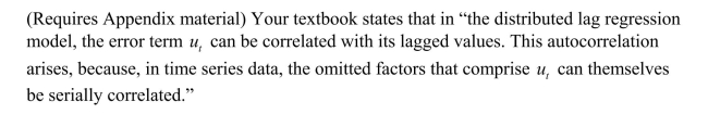
Your textbook mentions heteroskedasticity- and autocorrelation- consistent standard
errors.Explain why you should use this option in your regression package when
estimating the distributed lag regression model.What are the properties of the OLS
estimator in the presence of heteroskedasticity and autocorrelation in the error terms?
Explain why it is likely to find autocorrelation in time series data.If the errors are
autocorrelated, then why not simply adjust for autocorrelation by using some non-linear
estimation method such as Cochrane-Orcutt?
فتح الحزمة
افتح القفل للوصول البطاقات البالغ عددها 40 في هذه المجموعة.
فتح الحزمة
k this deck
32
(a)In the above expectation formation hypothesis, expectations are formed at the end of theperiod, say the
of December, if you had annual data.Give an intuitive explanation forthis process.
فتح الحزمة
افتح القفل للوصول البطاقات البالغ عددها 40 في هذه المجموعة.
فتح الحزمة
k this deck
33
The distributed lag model relating orange juice prices to the Orlando weather reported in
the text was of the form (a)Suppose that an agricultural economist tells you that a freeze in December is more
harmful than a freeze in the other months.How would you modify the regression to
incorporate this effect? How would you test for this December effect?
the text was of the form
(a)Suppose that an agricultural economist tells you that a freeze in December is moreharmful than a freeze in the other months.How would you modify the regression to
incorporate this effect? How would you test for this December effect?
فتح الحزمة
افتح القفل للوصول البطاقات البالغ عددها 40 في هذه المجموعة.
فتح الحزمة
k this deck
34
To estimate dynamic causal effects, your textbook presents the distributed lag regression
model, the autoregressive distributed lag model, and a quasi-difference representation of
the distributed lag model with autoregressive errors.Using a simple example, such as a
distributed lag model with only the current and past value of X and an AR(1)model for
the error term, discuss how these models are related.In each case suggest estimation
methods and evaluate the relative merit in using one rather than the other.
فتح الحزمة
افتح القفل للوصول البطاقات البالغ عددها 40 في هذه المجموعة.
فتح الحزمة
k this deck
35
GLS is consistent and BLUE if
فتح الحزمة
افتح القفل للوصول البطاقات البالغ عددها 40 في هذه المجموعة.
فتح الحزمة
k this deck
36
Money supply is linked to the monetary base by the money multiplier.Macroeconomic
textbooks tell you that the central bank cannot control the money supply, but it can
control the monetary base.As a result, you decide to specify a distributed lag equation of
the growth in the money supply on the growth in the monetary base.One of your peers
tells you that this is not a good idea for modeling the relationship between the two
variables.What does she mean?
فتح الحزمة
افتح القفل للوصول البطاقات البالغ عددها 40 في هذه المجموعة.
فتح الحزمة
k this deck
37
In the distributed lag model, the dynamic causal effect
A)is the sequence of coefficients on the current and lagged values of X.
B)is not the same as the dynamic multiplier.
C)is generated by choosing different truncation points for the HAC standard errors.
D)requires estimation of the model by Cochrane-Orcutt method.
A)is the sequence of coefficients on the current and lagged values of X.
B)is not the same as the dynamic multiplier.
C)is generated by choosing different truncation points for the HAC standard errors.
D)requires estimation of the model by Cochrane-Orcutt method.
فتح الحزمة
افتح القفل للوصول البطاقات البالغ عددها 40 في هذه المجموعة.
فتح الحزمة
k this deck
38
A model that attracted quite a bit of interest in macroeconomics in the 1970s was the St.
Louis model.The underlying idea was to calculate fiscal and monetary impact and long
run cumulative dynamic multipliers, by relating output (growth)to government
expenditure (growth)and money supply (growth).The assumption was that both
government expenditures and the money supply were exogenous.Estimation of a St.
Louis type model using quarterly data from 1960:I-1995:IV results in the following
output (HAC standard errors in parenthesis): where ygrowth is quarterly growth of real GDP, mgrowth is quarterly growth of real (a)Assuming that money and government expenditures are exogenous, what do the
coefficients represent? Calculate the h-period cumulative dynamic multipliers from these.
How can you test for the statistical significance of the cumulative dynamic multipliers
and the long-run cumulative dynamic multiplier?
Louis model.The underlying idea was to calculate fiscal and monetary impact and long
run cumulative dynamic multipliers, by relating output (growth)to government
expenditure (growth)and money supply (growth).The assumption was that both
government expenditures and the money supply were exogenous.Estimation of a St.
Louis type model using quarterly data from 1960:I-1995:IV results in the following
output (HAC standard errors in parenthesis):
where ygrowth is quarterly growth of real GDP, mgrowth is quarterly growth of real (a)Assuming that money and government expenditures are exogenous, what do thecoefficients represent? Calculate the h-period cumulative dynamic multipliers from these.
How can you test for the statistical significance of the cumulative dynamic multipliers
and the long-run cumulative dynamic multiplier?
فتح الحزمة
افتح القفل للوصول البطاقات البالغ عددها 40 في هذه المجموعة.
فتح الحزمة
k this deck
39
It has been argued that Canada's aggregate output growth and unemployment rates are
very sensitive to United States economic fluctuations, while the opposite is not true.
(a)A researcher uses a distributed lag model to estimate dynamic causal effects of U.S.
economic activity on Canada.The results (HAC standard errors in parenthesis)for the
sample period 1961:I-1995:IV are: where urcan is the Canadian unemployment rate, and urus is the United States
unemployment rate.
Calculate the long-run cumulative dynamic multiplier.
very sensitive to United States economic fluctuations, while the opposite is not true.
(a)A researcher uses a distributed lag model to estimate dynamic causal effects of U.S.
economic activity on Canada.The results (HAC standard errors in parenthesis)for the
sample period 1961:I-1995:IV are:
where urcan is the Canadian unemployment rate, and urus is the United Statesunemployment rate.
Calculate the long-run cumulative dynamic multiplier.
فتح الحزمة
افتح القفل للوصول البطاقات البالغ عددها 40 في هذه المجموعة.
فتح الحزمة
k this deck
40
One of the central predictions of neo-classical macroeconomic growth theory is that an
increase in the growth rate of the population causes at first a decline the growth rate of
real output per capita, but that subsequently the growth rate returns to its natural level,
itself determined by the rate of technological innovation.The intuition is that, if the
growth rate of the workforce increases, then more has to be saved to provide the new
workers with physical capital.However, accumulating capital takes time, so that output
per capita falls in the short run.
Under the assumption that population growth is exogenous, a number of regressions of
the growth rate of output per capita on current and lagged population growth were
performed, as reported below.(A constant was included in the regressions but is not
reported.HAC standard errors are in brackets.BIC is listed at the bottom of the table). (a)Which of these models is favored by the information criterion?
increase in the growth rate of the population causes at first a decline the growth rate of
real output per capita, but that subsequently the growth rate returns to its natural level,
itself determined by the rate of technological innovation.The intuition is that, if the
growth rate of the workforce increases, then more has to be saved to provide the new
workers with physical capital.However, accumulating capital takes time, so that output
per capita falls in the short run.
Under the assumption that population growth is exogenous, a number of regressions of
the growth rate of output per capita on current and lagged population growth were
performed, as reported below.(A constant was included in the regressions but is not
reported.HAC standard errors are in brackets.BIC is listed at the bottom of the table).
(a)Which of these models is favored by the information criterion? فتح الحزمة
افتح القفل للوصول البطاقات البالغ عددها 40 في هذه المجموعة.
فتح الحزمة
k this deck
فتح الحزمة
افتح القفل للوصول البطاقات البالغ عددها 40 في هذه المجموعة.


