Deck 14: Time Series: Descriptive Analyses, Models, and Forecasting Available on CD
ملء الشاشة (f)
سؤال
سؤال
سؤال
سؤال
سؤال
سؤال
سؤال
سؤال
سؤال
سؤال
سؤال
سؤال
سؤال
سؤال
سؤال
سؤال
سؤال
سؤال
سؤال
سؤال
سؤال
سؤال
سؤال
سؤال
سؤال
سؤال
سؤال
(Situation H) The prices of coffee, gasoline, and sugar for each month of 1983 are shown below in the table. 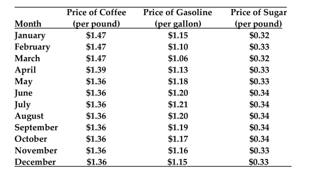
Using just the price of gasoline and a smoothing constant of lculate the exponentially smoothed value for March.
A) $1.102
B) $1.12
C) $1.076
D) $1.084
Using just the price of gasoline and a smoothing constant of
lculate the exponentially smoothed value for March.A) $1.102
B) $1.12
C) $1.076
D) $1.084
سؤال
سؤال
سؤال
سؤال
سؤال
سؤال
سؤال
سؤال
سؤال
سؤال
سؤال
سؤال
سؤال
سؤال
سؤال
سؤال
سؤال
سؤال
سؤال
سؤال
سؤال
The table below shows the price of a commodity for each of ten consecutive years. 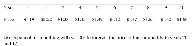
سؤال
سؤال
سؤال
سؤال
سؤال
سؤال
سؤال
سؤال
سؤال
سؤال
سؤال
سؤال
سؤال
سؤال
سؤال
سؤال
سؤال
سؤال
سؤال
سؤال
سؤال
سؤال
سؤال
سؤال
سؤال

فتح الحزمة
قم بالتسجيل لفتح البطاقات في هذه المجموعة!
Unlock Deck
Unlock Deck
1/73
العب
ملء الشاشة (f)
Deck 14: Time Series: Descriptive Analyses, Models, and Forecasting Available on CD
1
(Situation M) Fast food chains are closely watching what proposed legislation will do to consumption of "huge meals" in the United States. Researchers have accumulated statistics on the annual consumption of "huge for the past 25 years. The goal of the analysis is to use the past data to predict future consumption and then compare the predicted consumption to the actual consumption in those years.
-Propose a straight-line model that includes both a long-term trend and a seasonal component for the time series. Let the year in which the data was collected and let , and be dummy variables used to model a seasonal effect.
A)
B)
C)
D)
-Propose a straight-line model that includes both a long-term trend and a seasonal component for the time series. Let the year in which the data was collected and let , and be dummy variables used to model a seasonal effect.
A)
B)
C)
D)
2
(Situation G) The number of industrial and construction failures in the United States by the type of firm for the years 1985-1996 is given in the table.
-Using 1985 as the base period and using just construction failures, calculate the simple index for 1992.
A) 217.88
B) 46.43
C) 215.38
D) 487.20
-Using 1985 as the base period and using just construction failures, calculate the simple index for 1992.
A) 217.88
B) 46.43
C) 215.38
D) 487.20
215.38
3
(Situation J) The table lists the number (in millions) of Chevrolet passenger cars sold to dealers in the U.S. and Canada from 1980 to 1985.
-Using the exponential smoothing technique to the data from 1980 to 1985, forecast the number of Chevrolet passenger cars sold to U.S. and Canadian dealers in 1986 using
A) 2.448 million cars
B) 3.427 million cars
C) 4.882 million cars
D) 3.834 million cars
-Using the exponential smoothing technique to the data from 1980 to 1985, forecast the number of Chevrolet passenger cars sold to U.S. and Canadian dealers in 1986 using
A) 2.448 million cars
B) 3.427 million cars
C) 4.882 million cars
D) 3.834 million cars
2.448 million cars
4
(Situation L) A farmer's marketing cooperative recorded the volume of wheat harvested by its members from 1991 The cooperative is interested in detecting the long-term trend of the amount of wheat harvested. The data collected is
shown in the table.
-A forecast was obtained for the year 2005 and the corresponding 95% prediction interval was found to be (103, 107). Interpret this interval.
A) We are 95% confident that the volume of wheat harvested in 2005 will be between 103,000 and 107,000 bushels.
B) We are 95% confident that the mean volume of wheat harvested in all years will be between 103,000 and 107,000 bushels.
C) We expect the volume of wheat harvested to increase between 103,000 and 107,000 bushels from one year to the next.
D) We are 95% confident that the 2005 harvest will be between 103,000 and 107,000 bushels larger than the harvest in 2004.
فتح الحزمة
افتح القفل للوصول البطاقات البالغ عددها 73 في هذه المجموعة.
فتح الحزمة
k this deck
5
(Situation J) The table lists the number (in millions) of Chevrolet passenger cars sold to dealers in the U.S. and Canada from 1980 to 1985.
-Using a smoothing constant of ate the value of the exponentially smoothed series in 1983.
A) 1.289
B) 1.340
C) 1.228
D) 1.235
-Using a smoothing constant of ate the value of the exponentially smoothed series in 1983.
A) 1.289
B) 1.340
C) 1.228
D) 1.235
فتح الحزمة
افتح القفل للوصول البطاقات البالغ عددها 73 في هذه المجموعة.
فتح الحزمة
k this deck
6
The _______ generally describes fluctuations of the time series that are attributable to business and economic conditions.
A) seasonal variation
B) secular trend
C) cyclical effect
D) residual effect
A) seasonal variation
B) secular trend
C) cyclical effect
D) residual effect
فتح الحزمة
افتح القفل للوصول البطاقات البالغ عددها 73 في هذه المجموعة.
فتح الحزمة
k this deck
7
(Situation O) Using data from the post-Korean war period, an economist modeled annual consumption, , as a function of total labor income, , and total property income, , with the following results. Assume data for years were used in the analysis.
-For the situation above, give the rejection region for the Durbin-Watson test for autocorrelation of residuals. Use ? = 0.10.
A)
B) or
C)
D) or
-For the situation above, give the rejection region for the Durbin-Watson test for autocorrelation of residuals. Use ? = 0.10.
A)
B) or
C)
D) or
فتح الحزمة
افتح القفل للوصول البطاقات البالغ عددها 73 في هذه المجموعة.
فتح الحزمة
k this deck
8
Using just the wool prices and a smoothing constant w = 0.8, find the exponentially smoothed value for May.
A) 272.0
B) 275.0
C) 287.0
D) 276.9
A) 272.0
B) 275.0
C) 287.0
D) 276.9
فتح الحزمة
افتح القفل للوصول البطاقات البالغ عددها 73 في هذه المجموعة.
فتح الحزمة
k this deck
9
(Situation J) The table lists the number (in millions) of Chevrolet passenger cars sold to dealers in the U.S. and Canada from 1980 to 1985.
-Using the exponential smoothing technique to the data from 1980 to 1985, forecast the number of Chevrolet passenger cars to be sold to U.S. and Canadian dealers in 1986 using
A) 4.882 million cars
B) 3.427 million cars
C) 3.834 million cars
D) 2.448 million cars
-Using the exponential smoothing technique to the data from 1980 to 1985, forecast the number of Chevrolet passenger cars to be sold to U.S. and Canadian dealers in 1986 using
A) 4.882 million cars
B) 3.427 million cars
C) 3.834 million cars
D) 2.448 million cars
فتح الحزمة
افتح القفل للوصول البطاقات البالغ عددها 73 في هذه المجموعة.
فتح الحزمة
k this deck
10
(Situation F) The sales (in thousands of dollars) of automobiles by the three largest American automakers from 1986 through 1992 are shown in the table below.
-Using 1986 as the base year, find the simple composite index for 1990.
A) 85.53
B) 116.92
C) 65.81
D) 151.95
-Using 1986 as the base year, find the simple composite index for 1990.
A) 85.53
B) 116.92
C) 65.81
D) 151.95
فتح الحزمة
افتح القفل للوصول البطاقات البالغ عددها 73 في هذه المجموعة.
فتح الحزمة
k this deck
11
(Situation J) The table lists the number (in millions) of Chevrolet passenger cars sold to dealers in the U.S. and Canada from 1980 to 1985.
-The _______ is what remains of a time series value after the secular, cyclical, and seasonal components have been removed.
A) exponential effect
B) additive effect
C) residual effect
D) error effect
-The _______ is what remains of a time series value after the secular, cyclical, and seasonal components have been removed.
A) exponential effect
B) additive effect
C) residual effect
D) error effect
فتح الحزمة
افتح القفل للوصول البطاقات البالغ عددها 73 في هذه المجموعة.
فتح الحزمة
k this deck
12
The tendency of a series of values to increase or decrease over a long period of time is known as the _______ of a time series.
A) seasonal variation
B) cyclical fluctuation
C) secular trend
D) residual effect
A) seasonal variation
B) cyclical fluctuation
C) secular trend
D) residual effect
فتح الحزمة
افتح القفل للوصول البطاقات البالغ عددها 73 في هذه المجموعة.
فتح الحزمة
k this deck
13
(Situation G) The number of industrial and construction failures in the United States by the type of firm for the years 1985-1996 is given in the table.
-Using 1985 as the base year and using all five types of firms, calculate the simple composite index for 1995.
A) 217.88
B) 23.99
C) 476.49
D) 416.80
-Using 1985 as the base year and using all five types of firms, calculate the simple composite index for 1995.
A) 217.88
B) 23.99
C) 476.49
D) 416.80
فتح الحزمة
افتح القفل للوصول البطاقات البالغ عددها 73 في هذه المجموعة.
فتح الحزمة
k this deck
14
(Situation O) Using data from the post-Korean war period, an economist modeled annual consumption, as a function of total labor income, , and total property income, , with the following results. Assume data for were used in the analysis.
-For the situation above, set up the null and alternative hypotheses for testing for the presence of autocorrelation of residuals.
A)
: At least one
B) : No first-order autocorrelation
: Negative first-order autocorrelation
C) : No first-order autocorrelation
: Positive or Negative first-order autocorrelation
D) : No first-order autocorrelation
: Positive first-order autocorrelation
فتح الحزمة
افتح القفل للوصول البطاقات البالغ عددها 73 في هذه المجموعة.
فتح الحزمة
k this deck
15
(Situation L) A farmer's marketing cooperative recorded the volume of wheat harvested by its members from 1991-2004.
The cooperative is interested in detecting the long-term trend of the amount of wheat harvested. The data collected is shown in the table.
-Suppose the least squares regression equation is Interpret the estimate of in terms of the problem.
A) We expect the mean volume of wheat harvested to increase 2000 bushels from one year to the next.
B) We expect the volume of wheat harvested to increase 2000 bushels for each additional corporate member.
C) We expect the volume of wheat harvested to be 2000 bushels in any given year.
D) We expect to harvest 2000 bushels of wheat in 2005.
فتح الحزمة
افتح القفل للوصول البطاقات البالغ عددها 73 في هذه المجموعة.
فتح الحزمة
k this deck
16
(Situation L) A farmer's marketing cooperative recorded the volume of wheat harvested by its members from 1991 The cooperative is interested in detecting the long-term trend of the amount of wheat harvested. The data collected is
shown in the table.
-Suppose the least squares regression equation is . Use the regression model to forecast the harvest in 2005.
A) 110,000 bushels
B) 102,000 bushels
C) 105,000 bushels
D) 103,000 bushels
shown in the table.
-Suppose the least squares regression equation is . Use the regression model to forecast the harvest in 2005.
A) 110,000 bushels
B) 102,000 bushels
C) 105,000 bushels
D) 103,000 bushels
فتح الحزمة
افتح القفل للوصول البطاقات البالغ عددها 73 في هذه المجموعة.
فتح الحزمة
k this deck
17
(Situation M) Fast food chains are closely watching what proposed legislation will do to consumption of "huge meals" in the United States. Researchers have accumulated statistics on the annual consumption of "huge for the past 25 years. The goal of the analysis is to use the past data to predict future consumption and then compare the predicted consumption to the actual consumption in those years.
-To test for first-order autocorrelation, we use the _______ test.
A) Paasche
B) Laspeyres
C) Durbin-Watson
D) Wilcoxon
-To test for first-order autocorrelation, we use the _______ test.
A) Paasche
B) Laspeyres
C) Durbin-Watson
D) Wilcoxon
فتح الحزمة
افتح القفل للوصول البطاقات البالغ عددها 73 في هذه المجموعة.
فتح الحزمة
k this deck
18
(Situation O) Using data from the post-Korean war period, an economist modeled annual consumption, as a function of total labor income, , and total property income, , with the following results. Assume data for were used in the analysis.
-Is there evidence of positive autocorrelation of residuals in the consumption model presented above? Test using .
A) Yes, since the standard deviation is small.
B) Yes, since the Durbin-Watson statistic falls in the rejection region.
C) No, since the standard deviation is small.
D) No, since the Durbin-Watson statistic falls in the nonrejection region.
فتح الحزمة
افتح القفل للوصول البطاقات البالغ عددها 73 في هذه المجموعة.
فتح الحزمة
k this deck
19
(Situation M) Fast food chains are closely watching what proposed legislation will do to consumption of "huge meals" in the United States. Researchers have accumulated statistics on the annual consumption of "huge for the past 25 years. The goal of the analysis is to use the past data to predict future consumption and then compare the predicted consumption to the actual consumption in those years.
-Propose a straight-line model for the long-term trend of the time series. Do not include a seasonal component. Let the year in which the data was collected .
A)
B)
C)
D)
-Propose a straight-line model for the long-term trend of the time series. Do not include a seasonal component. Let the year in which the data was collected .
A)
B)
C)
D)
فتح الحزمة
افتح القفل للوصول البطاقات البالغ عددها 73 في هذه المجموعة.
فتح الحزمة
k this deck
20
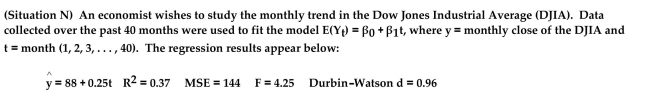
(Situation N) An economist wishes to study the monthly trend in the Dow Jones Industrial Average (DJIA). Data collected over the past 40 months were used to fit the model , monthly close of the DJIA and month . The regression results appear below:
-Since the data are recorded over time (months), there is a strong possibility that the residuals are positively correlated. How could you check for residual correlation using a graphical technique?
A) Plot the residuals against and look for a funnel shape.
B) Plot the residuals against and look for outliers.
C) Plot the residuals against and look for long runs of positive and negative residuals.
D) Plot the residuals against and look for a linear trend.
فتح الحزمة
افتح القفل للوصول البطاقات البالغ عددها 73 في هذه المجموعة.
فتح الحزمة
k this deck
21
فتح الحزمة
افتح القفل للوصول البطاقات البالغ عددها 73 في هذه المجموعة.
فتح الحزمة
k this deck
22
(Situation K) Foreign Exchange rates, the values of foreign currency in U.S. dollars, are important to investors and international travelers. The table lists the monthly foreign exchange rates of the British pound (in U.S. dollars per pound) for a certain year.
-Calculate the value of the exponentially smoothed series for April using a smoothing constant of
-Calculate the value of the exponentially smoothed series for April using a smoothing constant of
فتح الحزمة
افتح القفل للوصول البطاقات البالغ عددها 73 في هذه المجموعة.
فتح الحزمة
k this deck
23
(Situation J) The table lists the number (in millions) of Chevrolet passenger cars sold to dealers in the U.S. and Canada from 1980 to 1985.
-Using a smoothing constant of 0.30, calculate the value of the exponentially smoothed series in 1982.
A) 1.150
B) 1.289
C) 1.301
D) 1.425
-Using a smoothing constant of 0.30, calculate the value of the exponentially smoothed series in 1982.
A) 1.150
B) 1.289
C) 1.301
D) 1.425
فتح الحزمة
افتح القفل للوصول البطاقات البالغ عددها 73 في هذه المجموعة.
فتح الحزمة
k this deck
24
The _______ of a time series can account for fluctuations that recur during specific time periods.
A) secular trend
B) cyclical fluctuation
C) seasonal effect
D) residual effect
A) secular trend
B) cyclical fluctuation
C) seasonal effect
D) residual effect
فتح الحزمة
افتح القفل للوصول البطاقات البالغ عددها 73 في هذه المجموعة.
فتح الحزمة
k this deck
25
(Situation J) The table lists the number (in millions) of Chevrolet passenger cars sold to dealers in the U.S. and Canada from 1980 to 1985.
-Use the Holt forecasting model with trend to forecast the number of Chevrolet passenger cars sold to U.S. and Canadian dealers in 1990 using
A) 6.068 million cars
B) 8.72 million cars
C) 8.952 million cars
D) 6.39 million cars
-Use the Holt forecasting model with trend to forecast the number of Chevrolet passenger cars sold to U.S. and Canadian dealers in 1990 using
A) 6.068 million cars
B) 8.72 million cars
C) 8.952 million cars
D) 6.39 million cars
فتح الحزمة
افتح القفل للوصول البطاقات البالغ عددها 73 في هذه المجموعة.
فتح الحزمة
k this deck
26
Which of the following statements about the Durbin-Watson d-statistic is true?
A) It can assume any value between 0 and 2 .
B) It can assume any value between 0 and
C) It can assume any value between and 0 .
D) It can assume any value between and 4 .
A) It can assume any value between 0 and 2 .
B) It can assume any value between 0 and
C) It can assume any value between and 0 .
D) It can assume any value between and 4 .
فتح الحزمة
افتح القفل للوصول البطاقات البالغ عددها 73 في هذه المجموعة.
فتح الحزمة
k this deck
27
(Situation H) The prices of coffee, gasoline, and sugar for each month of 1983 are shown below in the table.
Using just the price of gasoline and a smoothing constant of lculate the exponentially smoothed value for March.
A) $1.102
B) $1.12
C) $1.076
D) $1.084
Using just the price of gasoline and a smoothing constant of
lculate the exponentially smoothed value for March.A) $1.102
B) $1.12
C) $1.076
D) $1.084
فتح الحزمة
افتح القفل للوصول البطاقات البالغ عددها 73 في هذه المجموعة.
فتح الحزمة
k this deck
28
Consider the monthly time series shown in the table.
a. Use the values of in the table to forecast the values of for the next two months, using simple exponential smoothing with .
b. Use the Holt model with and to forecast the values of for the next two months.
a. Use the values of in the table to forecast the values of for the next two months, using simple exponential smoothing with .
b. Use the Holt model with and to forecast the values of for the next two months.
فتح الحزمة
افتح القفل للوصول البطاقات البالغ عددها 73 في هذه المجموعة.
فتح الحزمة
k this deck
29
(Situation G) The number of industrial and construction failures in the United States by the type of firm for the years 1985-1996 is given in the table.
-Using just the wholesale trade failures and a smoothing constant , calculate the exponentially smoothed value for 1988.
A) 1015.6
B) 798.4
C) 932.9
D) 845
-Using just the wholesale trade failures and a smoothing constant , calculate the exponentially smoothed value for 1988.
A) 1015.6
B) 798.4
C) 932.9
D) 845
فتح الحزمة
افتح القفل للوصول البطاقات البالغ عددها 73 في هذه المجموعة.
فتح الحزمة
k this deck
30
Consider the table below which displays the price of a commodity for six consecutive
years.
a. Calculate the values in the exponentially smoothed series using .
b. Calculate the forecast errors for Years 7-10 if the actual values in those years are 262, 264, 263, 266 respectively.
c. Calculate MAD, MAPE, and RMSE, using the forecast errors for Years 7-10.
years.
a. Calculate the values in the exponentially smoothed series using .
b. Calculate the forecast errors for Years 7-10 if the actual values in those years are 262, 264, 263, 266 respectively.
c. Calculate MAD, MAPE, and RMSE, using the forecast errors for Years 7-10.
فتح الحزمة
افتح القفل للوصول البطاقات البالغ عددها 73 في هذه المجموعة.
فتح الحزمة
k this deck
31
Consider the actual values Y and forecast values F given in the table below. Calculate the root mean squared error (RMSE) of the forecasts.
A) 0.90
B) 0.30
C) 0.37
D) 1.42
A) 0.90
B) 0.30
C) 0.37
D) 1.42
فتح الحزمة
افتح القفل للوصول البطاقات البالغ عددها 73 في هذه المجموعة.
فتح الحزمة
k this deck
32
(Situation J) The table lists the number (in millions) of Chevrolet passenger cars sold to dealers in the U.S. and Canada from 1980 to 1985.
-Use the Holt forecasting model with trend to forecast the number of Chevrolet passenger cars sold to U.S. and Canadian dealers in 1990 using
A) 8.952 million cars
B) 8.72 million cars
C) 6.068 million cars
D) 6.39 million cars
-Use the Holt forecasting model with trend to forecast the number of Chevrolet passenger cars sold to U.S. and Canadian dealers in 1990 using
A) 8.952 million cars
B) 8.72 million cars
C) 6.068 million cars
D) 6.39 million cars
فتح الحزمة
افتح القفل للوصول البطاقات البالغ عددها 73 في هذه المجموعة.
فتح الحزمة
k this deck
33
Consider the monthly time series shown in the table.
a. Use the method of least squares to fit the model to the data. Write the prediction equation.
b. Construct a residual plot for the model.
c. Is there evidence of a cyclical component? Explain.
a. Use the method of least squares to fit the model to the data. Write the prediction equation.
b. Construct a residual plot for the model.
c. Is there evidence of a cyclical component? Explain.
فتح الحزمة
افتح القفل للوصول البطاقات البالغ عددها 73 في هذه المجموعة.
فتح الحزمة
k this deck
34
Consider the actual values Y and forecast values F given in the table below. Calculate the mean absolute deviation (MAD) of the forecasts.
A) 1.42
B) 0.90
C) 0.30
D) 0.37
A) 1.42
B) 0.90
C) 0.30
D) 0.37
فتح الحزمة
افتح القفل للوصول البطاقات البالغ عددها 73 في هذه المجموعة.
فتح الحزمة
k this deck
35
A(n) _______ is a number that measures the change in a variable over time relative to the value of the variable during a base period.
A) index number
B) exponential smoothing constant
C) residual value
D) time series
A) index number
B) exponential smoothing constant
C) residual value
D) time series
فتح الحزمة
افتح القفل للوصول البطاقات البالغ عددها 73 في هذه المجموعة.
فتح الحزمة
k this deck
36
(Situation K) Foreign Exchange rates, the values of foreign currency in U.S. dollars, are important to investors and international travelers. The table lists the monthly foreign exchange rates of the British pound (in U.S. dollars per pound) for a certain year.
-Consider the table below which displays the price of a commodity for six consecutive
years.
a. prediction equation.
b. Calculate the residuals and construct a residual plot.
c. Calculate the Durbin Watson d statistic.
-Consider the table below which displays the price of a commodity for six consecutive
years.
a. prediction equation.
b. Calculate the residuals and construct a residual plot.
c. Calculate the Durbin Watson d statistic.
فتح الحزمة
افتح القفل للوصول البطاقات البالغ عددها 73 في هذه المجموعة.
فتح الحزمة
k this deck
37
Consider the actual values Y and forecast values F given in the table below. Calculate the mean absolute percentage error (MAPE) of the forecasts.
A) 0.37
B) 0.30
C) 1.42
D) 0.90
A) 0.37
B) 0.30
C) 1.42
D) 0.90
فتح الحزمة
افتح القفل للوصول البطاقات البالغ عددها 73 في هذه المجموعة.
فتح الحزمة
k this deck
38
(Situation L) A farmer's marketing cooperative recorded the volume of wheat harvested by its members from 1991
The cooperative is interested in detecting the long-term trend of the amount of wheat harvested. The data collected is shown in the table.
-Find the least squares prediction equation for the model .
A)
B)
C)
D)
The cooperative is interested in detecting the long-term trend of the amount of wheat harvested. The data collected is shown in the table.
-Find the least squares prediction equation for the model .
A)
B)
C)
D)
فتح الحزمة
افتح القفل للوصول البطاقات البالغ عددها 73 في هذه المجموعة.
فتح الحزمة
k this deck
39
(Situation F) The sales (in thousands of dollars) of automobiles by the three largest American automakers from 1986
through 1992 are shown in the table below.
-Using 1986 as the base year, and only using the Chrysler sales data, find the simple index for 1992.
A) 102.49
B) 83.26
C) 97.57
D) 120.10
through 1992 are shown in the table below.
-Using 1986 as the base year, and only using the Chrysler sales data, find the simple index for 1992.
A) 102.49
B) 83.26
C) 97.57
D) 120.10
فتح الحزمة
افتح القفل للوصول البطاقات البالغ عددها 73 في هذه المجموعة.
فتح الحزمة
k this deck
40
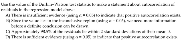
(Situation N) An economist wishes to study the monthly trend in the Dow Jones Industrial Average (DJIA). Data collected over the past 40 months were used to fit the model , where monthly close of the DJIA and month . The regression results appear below:
-What is the value of the test statistic for testing whether autocorrelation exists in the data?
A) 4.25
B) 0.25
C) 0.37
D) 0.96
-What is the value of the test statistic for testing whether autocorrelation exists in the data?
A) 4.25
B) 0.25
C) 0.37
D) 0.96
فتح الحزمة
افتح القفل للوصول البطاقات البالغ عددها 73 في هذه المجموعة.
فتح الحزمة
k this deck
41
It is common to use dummy variables to describe seasonal differences in a time series.
فتح الحزمة
افتح القفل للوصول البطاقات البالغ عددها 73 في هذه المجموعة.
فتح الحزمة
k this deck
42
(Situation J) The table lists the number (in millions) of Chevrolet passenger cars sold to dealers in the U.S. and Canada from 1980 to 1985.
-Using a smoothing constant of 0.70, calculate the value of the exponentially smoothed series in 1985.
-Using a smoothing constant of 0.70, calculate the value of the exponentially smoothed series in 1985.
فتح الحزمة
افتح القفل للوصول البطاقات البالغ عددها 73 في هذه المجموعة.
فتح الحزمة
k this deck
43
The printout below shows a regression analysis for a time series that included 20 observations.
Regression Analysis: C2 versus C1
The regression equation is
Analysis of Variance
Locate the Durbin-Watson d-statistic and test the null hypothesis that there is no autocorrelation of residuals. Use .
Regression Analysis: C2 versus C1
The regression equation is
Analysis of Variance
Locate the Durbin-Watson d-statistic and test the null hypothesis that there is no autocorrelation of residuals. Use .
فتح الحزمة
افتح القفل للوصول البطاقات البالغ عددها 73 في هذه المجموعة.
فتح الحزمة
k this deck
44
Since the theoretical distributional properties of the forecast errors with smoothing methods are unknown, many analysts regard smoothing methods as descriptive procedures rather than inferential procedures.
فتح الحزمة
افتح القفل للوصول البطاقات البالغ عددها 73 في هذه المجموعة.
فتح الحزمة
k this deck
45
The Laspeyres index is a weighted index while the Paasche index is not weighted.
فتح الحزمة
افتح القفل للوصول البطاقات البالغ عددها 73 في هذه المجموعة.
فتح الحزمة
k this deck
46
A composite index number represents combinations of the prices or quantities of several commodities.
فتح الحزمة
افتح القفل للوصول البطاقات البالغ عددها 73 في هذه المجموعة.
فتح الحزمة
k this deck
47
Fourth-order autocorrelation in a quarterly time series may indicate seasonality.
فتح الحزمة
افتح القفل للوصول البطاقات البالغ عددها 73 في هذه المجموعة.
فتح الحزمة
k this deck
48
The table below shows the price of a commodity for each of ten consecutive years.
فتح الحزمة
افتح القفل للوصول البطاقات البالغ عددها 73 في هذه المجموعة.
فتح الحزمة
k this deck
49
The d-test requires that the residuals be normally distributed.
فتح الحزمة
افتح القفل للوصول البطاقات البالغ عددها 73 في هذه المجموعة.
فتح الحزمة
k this deck
50
The table below shows the price of a commodity for each of ten consecutive years.
a. Using Year 1 as the base period, calculate the simple index for the price of the commodity for each year.
b. Plot the simple indexes for years 1-10.
c. Use the simple index to interpret the trend in the price of the commodity.
a. Using Year 1 as the base period, calculate the simple index for the price of the commodity for each year.
b. Plot the simple indexes for years 1-10.
c. Use the simple index to interpret the trend in the price of the commodity.
فتح الحزمة
افتح القفل للوصول البطاقات البالغ عددها 73 في هذه المجموعة.
فتح الحزمة
k this deck
51
The table below shows the prices and quantities of three commodities for six consecutive
years.
a. Compute the Laspeyres price index for the six-year period, using Year 1 as the base period.
b. Compute the Paasche price index for the six-year period, using Year 1 as the base period.
c. Plot the Laspeyres and Paasche indexes on the same graph. Comment on the
differences.
years.
a. Compute the Laspeyres price index for the six-year period, using Year 1 as the base period.
b. Compute the Paasche price index for the six-year period, using Year 1 as the base period.
c. Plot the Laspeyres and Paasche indexes on the same graph. Comment on the
differences.
فتح الحزمة
افتح القفل للوصول البطاقات البالغ عددها 73 في هذه المجموعة.
فتح الحزمة
k this deck
52
Consider the monthly time series shown in the table. a. Calculate the values in the exponentially smoothed series using w b. Graph the time series and the exponentially smoothed series on the same graph.
فتح الحزمة
افتح القفل للوصول البطاقات البالغ عددها 73 في هذه المجموعة.
فتح الحزمة
k this deck
53
Consider the monthly time series shown in the table. a. Use the method of least squares to fit the mo t to the data. Write the prediction equation.
b. Use the prediction equation to obtain forecasts for the next two months.
c. Find 95% forecast intervals for the next two months.
b. Use the prediction equation to obtain forecasts for the next two months.
c. Find 95% forecast intervals for the next two months.
فتح الحزمة
افتح القفل للوصول البطاقات البالغ عددها 73 في هذه المجموعة.
فتح الحزمة
k this deck
54
The exponential smoothing constant can be any number between 0 and 100.
فتح الحزمة
افتح القفل للوصول البطاقات البالغ عددها 73 في هذه المجموعة.
فتح الحزمة
k this deck
55
We plot time series residuals against observed values of Y to determine whether a cyclical component is apparent.
فتح الحزمة
افتح القفل للوصول البطاقات البالغ عددها 73 في هذه المجموعة.
فتح الحزمة
k this deck
56
Consider the table below which displays the price of a commodity for six consecutive years. a. Use the Holt model to forecast values for Years 7-10 using and .
b. Calculate the forecast errors for Years 7-10 if the actual values in those years are 263, 267, 269, 268 respectively.
c. Calculate MAD, MAPE, and RMSE, using the forecast errors for Years 7-10.
b. Calculate the forecast errors for Years 7-10 if the actual values in those years are 263, 267, 269, 268 respectively.
c. Calculate MAD, MAPE, and RMSE, using the forecast errors for Years 7-10.
فتح الحزمة
افتح القفل للوصول البطاقات البالغ عددها 73 في هذه المجموعة.
فتح الحزمة
k this deck
57
(Situation F) The sales (in thousands of dollars) of automobiles by the three largest American automakers from 1986 through 1992 are shown in the table below.
-Using 1986 as the base year, find the simple composite index for 1992.
-Using 1986 as the base year, find the simple composite index for 1992.
فتح الحزمة
افتح القفل للوصول البطاقات البالغ عددها 73 في هذه المجموعة.
فتح الحزمة
k this deck
58
Price indexes measure changes in the price of a commodity or group of commodities over time.
فتح الحزمة
افتح القفل للوصول البطاقات البالغ عددها 73 في هذه المجموعة.
فتح الحزمة
k this deck
59
Consider the table below which displays the price of a commodity for six consecutive years.
a. Use the method of least squares to fit the model to the data. Write the prediction equation.
b. Use the prediction equation to obtain forecasts of the prices in years 7 and 8 .
c. Find prediction intervals for years 7 and 8 .
a. Use the method of least squares to fit the model to the data. Write the prediction equation.
b. Use the prediction equation to obtain forecasts of the prices in years 7 and 8 .
c. Find prediction intervals for years 7 and 8 .
فتح الحزمة
افتح القفل للوصول البطاقات البالغ عددها 73 في هذه المجموعة.
فتح الحزمة
k this deck
60
Retail sales for a home improvement store in quarters 1-4 over a five-year period are shown (in millions of dollars) in the table below. a. Write a regression model that contains trend and seasonal components to describe the sales data.
b. Use least squares regression to fit the model.
c. Use the regression model to forecast the quarterly sales during Year 6. Give 95% prediction intervals for the forecasts.
b. Use least squares regression to fit the model.
c. Use the regression model to forecast the quarterly sales during Year 6. Give 95% prediction intervals for the forecasts.
فتح الحزمة
افتح القفل للوصول البطاقات البالغ عددها 73 في هذه المجموعة.
فتح الحزمة
k this deck
61
The least squares model is an excellent choice for forecasting time series since it works particularly well outside the region of known observations.
فتح الحزمة
افتح القفل للوصول البطاقات البالغ عددها 73 في هذه المجموعة.
فتح الحزمة
k this deck
62
Smaller values of the trend smoothing constant v assign more weight to the most recent trend of the series and less to past trends.
فتح الحزمة
افتح القفل للوصول البطاقات البالغ عددها 73 في هذه المجموعة.
فتح الحزمة
k this deck
63
One of the major weaknesses of exponential smoothing is that it is not easily adapted to forecasting.
فتح الحزمة
افتح القفل للوصول البطاقات البالغ عددها 73 في هذه المجموعة.
فتح الحزمة
k this deck
64
Smoothing techniques are used to remove rapid fluctuations in a time series so the general trend can be seen.
فتح الحزمة
افتح القفل للوصول البطاقات البالغ عددها 73 في هذه المجموعة.
فتح الحزمة
k this deck
65
With N time periods in your data, a good rule of thumb is to forecast ahead no more than 2N time periods.
فتح الحزمة
افتح القفل للوصول البطاقات البالغ عددها 73 في هذه المجموعة.
فتح الحزمة
k this deck
66
A major advantage of forecasting with smoothing techniques is that the standard deviation of the forecast errors is known prior to observing the future values.
فتح الحزمة
افتح القفل للوصول البطاقات البالغ عددها 73 في هذه المجموعة.
فتح الحزمة
k this deck
67
The Holt forecasting model consists of both an exponentially smoothed component and a trend component.
فتح الحزمة
افتح القفل للوصول البطاقات البالغ عددها 73 في هذه المجموعة.
فتح الحزمة
k this deck
68
The straight-line regression model accounts for both the secular trend and the cyclical effect in a time series.
فتح الحزمة
افتح القفل للوصول البطاقات البالغ عددها 73 في هذه المجموعة.
فتح الحزمة
k this deck
69
The exponentially smoothed forecast takes into account both changes in trend and seasonality.
فتح الحزمة
افتح القفل للوصول البطاقات البالغ عددها 73 في هذه المجموعة.
فتح الحزمة
k this deck
70
The value of the Durbin-Watson d-statistic always falls in the interval from 0 to 1.
فتح الحزمة
افتح القفل للوصول البطاقات البالغ عددها 73 في هذه المجموعة.
فتح الحزمة
k this deck
71
The choice of exponential smoothing constant w has little or no effect on forecast values found using exponential smoothing.
فتح الحزمة
افتح القفل للوصول البطاقات البالغ عددها 73 في هذه المجموعة.
فتح الحزمة
k this deck
72
The Laspeyres index uses the purchase quantities of the period as weights.
فتح الحزمة
افتح القفل للوصول البطاقات البالغ عددها 73 في هذه المجموعة.
فتح الحزمة
k this deck
73
Smaller choices of the exponential smoothing constant w assign more weight to the current value of the series and yield a smoother series.
فتح الحزمة
افتح القفل للوصول البطاقات البالغ عددها 73 في هذه المجموعة.
فتح الحزمة
k this deck
فتح الحزمة
افتح القفل للوصول البطاقات البالغ عددها 73 في هذه المجموعة.


