Deck 14: Introduction to Multiple
ملء الشاشة (f)
سؤال
SCENARIO 14-3
An economist is interested to see how consumption for an economy (in $ billions) is influenced by
gross domestic product ($ billions) and aggregate price (consumer price index). The Microsoft Excel
output of this regression is partially reproduced below.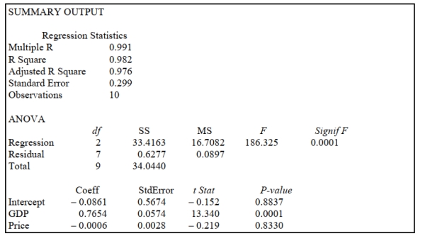
Referring to Scenario 14-3, what is the estimated mean consumption level for an economy with GDP equal to $2 billion and an aggregate price index of 90?
A) $1.39 billion
B) $2.89 billion
C) $4.75 billion
D) $9.45 billion
سؤال
SCENARIO 14-1 A manager of a product sales group believes the number of sales made by an employee depends on how many years that employee has been with the company and how he/she scored on a business aptitude test . A random sample of 8 employees provides the following:
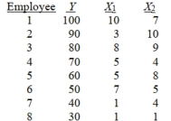
-Referring to Scenario 14-1, if an employee who had been with the company 5 years scored a 9 on the aptitude test, what would his estimated expected sales be?
A) 79.09
B) 60.88
C) 55.62
D) 17.98
-Referring to Scenario 14-1, if an employee who had been with the company 5 years scored a 9 on the aptitude test, what would his estimated expected sales be?
A) 79.09
B) 60.88
C) 55.62
D) 17.98
سؤال
SCENARIO 14-2 A professor of industrial relations believes that an individual's wage rate at a factory depends on his performance rating and the number of economics courses the employee successfully completed in college . The professor randomly selects 6 workers and collects the following information:
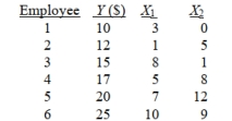
-Referring to Scenario 14-2, an employee who took 12 economics courses scores 10 on the performance rating. What is her estimated expected wage rate?
A) 10.90
B) 12.20
C) 24.87
D) 25.70
-Referring to Scenario 14-2, an employee who took 12 economics courses scores 10 on the performance rating. What is her estimated expected wage rate?
A) 10.90
B) 12.20
C) 24.87
D) 25.70
سؤال
SCENARIO 14-2 A professor of industrial relations believes that an individual's wage rate at a factory depends on his performance rating and the number of economics courses the employee successfully completed in college . The professor randomly selects 6 workers and collects the following information:
-Referring to Scenario 14-2, for these data, what is the value for the regression constant, b0?
A) 0.616
B) 1.054
C) 6.932
D) 9.103
-Referring to Scenario 14-2, for these data, what is the value for the regression constant, b0?
A) 0.616
B) 1.054
C) 6.932
D) 9.103
سؤال
In a multiple regression model, the value of the coefficient of multiple determination 
سؤال
SCENARIO 14-3
An economist is interested to see how consumption for an economy (in $ billions) is influenced by
gross domestic product ($ billions) and aggregate price (consumer price index). The Microsoft Excel
output of this regression is partially reproduced below.
Referring to Scenario 14-3, the p-value for GDP is
A) 0.05
B) 0.01
C) 0.001
D) None of the above.
سؤال
SCENARIO 14-2 A professor of industrial relations believes that an individual's wage rate at a factory depends on his performance rating and the number of economics courses the employee successfully completed in college . The professor randomly selects 6 workers and collects the following information:
-Referring to Scenario 14-2, for these data, what is the estimated coefficient for the number of economics courses taken, ?
A) 0.616
B) 1.054
C) 6.932
D) 9.103
-Referring to Scenario 14-2, for these data, what is the estimated coefficient for the number of economics courses taken, ?
A) 0.616
B) 1.054
C) 6.932
D) 9.103
سؤال
SCENARIO 14-3
An economist is interested to see how consumption for an economy (in $ billions) is influenced by
gross domestic product ($ billions) and aggregate price (consumer price index). The Microsoft Excel
output of this regression is partially reproduced below.
-Referring to Scenario 14-3, when the economist used a simple linear regression model with consumption as the dependent variable and GDP as the independent variable, he obtained an value of 0.971. What additional percentage of the total variation of consumption has been
Explained by including aggregate prices in the multiple regression?
A) 98.2
B) 11.1
C) 2.8
D) 1.1
سؤال
SCENARIO 14-1 A manager of a product sales group believes the number of sales made by an employee depends on how many years that employee has been with the company and how he/she scored on a business aptitude test . A random sample of 8 employees provides the following:
-Referring to Scenario 14-1, for these data, what is the value for the regression constant, b0?
A) 0.998
B) 3.103
C) 4.698
D) 21.293
-Referring to Scenario 14-1, for these data, what is the value for the regression constant, b0?
A) 0.998
B) 3.103
C) 4.698
D) 21.293
سؤال
SCENARIO 14-3
An economist is interested to see how consumption for an economy (in $ billions) is influenced by
gross domestic product ($ billions) and aggregate price (consumer price index). The Microsoft Excel
output of this regression is partially reproduced below.
Referring to Scenario 14-3, what is the predicted consumption level for an economy with GDP equal to $4 billion and an aggregate price index of 150?
A) $1.39 billion
B) $2.89 billion
C) $4.75 billion
D) $9.45 billion
سؤال
سؤال
SCENARIO 14-3
An economist is interested to see how consumption for an economy (in $ billions) is influenced by
gross domestic product ($ billions) and aggregate price (consumer price index). The Microsoft Excel
output of this regression is partially reproduced below.
Referring to Scenario 14-3, the p-value for the regression model as a whole is
A) 0.05
B) 0.01
C) 0.001
D) None of the above.
سؤال
SCENARIO 14-2 A professor of industrial relations believes that an individual's wage rate at a factory depends on his performance rating and the number of economics courses the employee successfully completed in college . The professor randomly selects 6 workers and collects the following information:
-Referring to Scenario 14-2, suppose an employee had never taken an economics course and managed to score a 5 on his performance rating. What is his estimated expected wage rate?
A) 10.90
B) 12.20
C) 17.23
D) 25.11
-Referring to Scenario 14-2, suppose an employee had never taken an economics course and managed to score a 5 on his performance rating. What is his estimated expected wage rate?
A) 10.90
B) 12.20
C) 17.23
D) 25.11
سؤال
SCENARIO 14-1 A manager of a product sales group believes the number of sales made by an employee depends on how many years that employee has been with the company and how he/she scored on a business aptitude test . A random sample of 8 employees provides the following:
-Referring to Scenario 14-1, for these data, what is the estimated coefficient for the variable representing years an employee has been with the company, b1?
A) 0.998
B) 3.103
C) 4.698
D) 21.293
-Referring to Scenario 14-1, for these data, what is the estimated coefficient for the variable representing years an employee has been with the company, b1?
A) 0.998
B) 3.103
C) 4.698
D) 21.293
سؤال
SCENARIO 14-2 A professor of industrial relations believes that an individual's wage rate at a factory depends on his performance rating and the number of economics courses the employee successfully completed in college . The professor randomly selects 6 workers and collects the following information:
-Referring to Scenario 14-2, for these data, what is the estimated coefficient for performance rating, b1?
A) 0.616
B) 1.054
C) 6.932
D) 9.103
-Referring to Scenario 14-2, for these data, what is the estimated coefficient for performance rating, b1?
A) 0.616
B) 1.054
C) 6.932
D) 9.103
سؤال
SCENARIO 14-3
An economist is interested to see how consumption for an economy (in $ billions) is influenced by
gross domestic product ($ billions) and aggregate price (consumer price index). The Microsoft Excel
output of this regression is partially reproduced below.
Referring to Scenario 14-3, the p-value for the aggregated price index is
A) 0.05
B) 0.01
C) 0.001
D) None of the above.
سؤال
SCENARIO 14-1 A manager of a product sales group believes the number of sales made by an employee depends on how many years that employee has been with the company and how he/she scored on a business aptitude test . A random sample of 8 employees provides the following:
-Referring to Scenario 14-1, for these data, what is the estimated coefficient for the variable representing scores on the aptitude test, b2?
A) 0.998
B) 3.103
C) 4.698
D) 21.293
-Referring to Scenario 14-1, for these data, what is the estimated coefficient for the variable representing scores on the aptitude test, b2?
A) 0.998
B) 3.103
C) 4.698
D) 21.293
سؤال
SCENARIO 14-2 A professor of industrial relations believes that an individual's wage rate at a factory depends on his performance rating and the number of economics courses the employee successfully completed in college . The professor randomly selects 6 workers and collects the following information:
-The variation attributable to factors other than the relationship between the independent variables and the explained variable in a regression analysis is represented by
A) regression sum of squares.
B) error sum of squares.
C) total sum of squares.
D) regression mean squares.
-The variation attributable to factors other than the relationship between the independent variables and the explained variable in a regression analysis is represented by
A) regression sum of squares.
B) error sum of squares.
C) total sum of squares.
D) regression mean squares.
سؤال
SCENARIO 14-3
An economist is interested to see how consumption for an economy (in $ billions) is influenced by
gross domestic product ($ billions) and aggregate price (consumer price index). The Microsoft Excel
output of this regression is partially reproduced below.
Referring to Scenario 14-3, one economy in the sample had an aggregate consumption level of $3 billion, a GDP of $3.5 billion, and an aggregate price level of 125. What is the residual for this
Data point?
A) $2.52 billion
B) $0.48 billion
C) - $1.33 billion
D) - $2.52 billion
سؤال
SCENARIO 14-3
An economist is interested to see how consumption for an economy (in $ billions) is influenced by
gross domestic product ($ billions) and aggregate price (consumer price index). The Microsoft Excel
output of this regression is partially reproduced below.
Referring to Scenario 14-3, what is the estimated mean consumption level for an economy with GDP equal to $4 billion and an aggregate price index of 150?
A) $1.39 billion
B) $2.89 billion
C) $4.75 billion
D) $9.45 billion
سؤال
SCENARIO 14-4
A real estate builder wishes to determine how house size (House) is influenced by family income
(Income) and family size (Size). House size is measured in hundreds of square feet and income is
measured in thousands of dollars. The builder randomly selected 50 families and ran the multiple
regression. Partial Microsoft Excel output is provided below: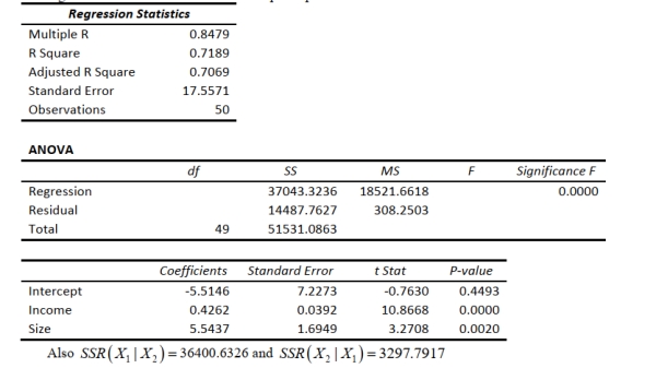
Referring to Scenario 14-4, suppose the builder wants to test whether the coefficient on Income is significantly different from 0. What is the value of the relevant t-statistic?
A) -0.7630
B) 3.2708
C) 10.8668
D) 60.0864
سؤال
SCENARIO 14-4
A real estate builder wishes to determine how house size (House) is influenced by family income
(Income) and family size (Size). House size is measured in hundreds of square feet and income is
measured in thousands of dollars. The builder randomly selected 50 families and ran the multiple
regression. Partial Microsoft Excel output is provided below:
Referring to Scenario 14-4, what is the predicted house size (in hundreds of square feet) for an
individual earning an annual income of $40,000 and having a family size of 4?
سؤال
SCENARIO 14-4
A real estate builder wishes to determine how house size (House) is influenced by family income
(Income) and family size (Size). House size is measured in hundreds of square feet and income is
measured in thousands of dollars. The builder randomly selected 50 families and ran the multiple
regression. Partial Microsoft Excel output is provided below:
Referring to Scenario 14-4, what fraction of the variability in house size is explained by income and size of family?
A) 17.56%
B) 70.69%
C) 71.89%
D) 84.79%
سؤال
SCENARIO 14-4
A real estate builder wishes to determine how house size (House) is influenced by family income
(Income) and family size (Size). House size is measured in hundreds of square feet and income is
measured in thousands of dollars. The builder randomly selected 50 families and ran the multiple
regression. Partial Microsoft Excel output is provided below:
Referring to Scenario 14-4, one individual in the sample had an annual income of $40,000 and a
family size of 1. This individual owned a home with an area of 1,000 square feet (House =
10.00). What is the residual (in hundreds of square feet) for this data point?
سؤال
SCENARIO 14-3
An economist is interested to see how consumption for an economy (in $ billions) is influenced by
gross domestic product ($ billions) and aggregate price (consumer price index). The Microsoft Excel
output of this regression is partially reproduced below.
Referring to Scenario 14-3, to test for the significance of the coefficient on gross domestic product, the p-value is
A) 0.0001
B) 0.8330
C) 0.8837
D) 0.9999
سؤال
SCENARIO 14-4
A real estate builder wishes to determine how house size (House) is influenced by family income
(Income) and family size (Size). House size is measured in hundreds of square feet and income is
measured in thousands of dollars. The builder randomly selected 50 families and ran the multiple
regression. Partial Microsoft Excel output is provided below:
Referring to Scenario 14-4, which of the following values for the level of significance is the smallest for which at least one explanatory variable is significant individually?
A) 0.005
B) 0.010
C) 0.025
D) 0.050
سؤال
SCENARIO 14-4
A real estate builder wishes to determine how house size (House) is influenced by family income
(Income) and family size (Size). House size is measured in hundreds of square feet and income is
measured in thousands of dollars. The builder randomly selected 50 families and ran the multiple
regression. Partial Microsoft Excel output is provided below:
-Referring to Scenario 14-4, when the builder used a simple linear regression model with house size (House) as the dependent variable and family size (Size) as the independent variable, he
Obtained an value of 1.25%. What additional percentage of the total variation in house size has
Been explained by including income in the multiple regression?
A) 15.00%
B) 70.64%
C) 71.50%
D) 73.62%
سؤال
SCENARIO 14-3
An economist is interested to see how consumption for an economy (in $ billions) is influenced by
gross domestic product ($ billions) and aggregate price (consumer price index). The Microsoft Excel
output of this regression is partially reproduced below.
Referring to Scenario 14-3, to test whether aggregate price index has a positive impact on consumption, the p-value is
A) 0.0001
B) 0.4165
C) 0.5835
D) 0.8330
سؤال
SCENARIO 14-4
A real estate builder wishes to determine how house size (House) is influenced by family income
(Income) and family size (Size). House size is measured in hundreds of square feet and income is
measured in thousands of dollars. The builder randomly selected 50 families and ran the multiple
regression. Partial Microsoft Excel output is provided below:
Referring to Scenario 14-4, what annual income (in thousands of dollars) would an individual
with a family size of 9 need to attain a predicted 5,000 square foot home (House = 50)?
سؤال
SCENARIO 14-4
A real estate builder wishes to determine how house size (House) is influenced by family income
(Income) and family size (Size). House size is measured in hundreds of square feet and income is
measured in thousands of dollars. The builder randomly selected 50 families and ran the multiple
regression. Partial Microsoft Excel output is provided below:
Referring to Scenario 14-4, which of the following values for the level of significance is the smallest for which each explanatory variable is significant individually?
A) 0.001
B) 0.010
C) 0.025
D) 0.050
سؤال
SCENARIO 14-4
A real estate builder wishes to determine how house size (House) is influenced by family income
(Income) and family size (Size). House size is measured in hundreds of square feet and income is
measured in thousands of dollars. The builder randomly selected 50 families and ran the multiple
regression. Partial Microsoft Excel output is provided below:
Referring to Scenario 14-4, what annual income (in thousands of dollars) would an individual
with a family size of 4 need to attain a predicted 10,000 square foot home (House = 100)?
سؤال
SCENARIO 14-3
An economist is interested to see how consumption for an economy (in $ billions) is influenced by
gross domestic product ($ billions) and aggregate price (consumer price index). The Microsoft Excel
output of this regression is partially reproduced below.
Referring to Scenario 14-3, one economy in the sample had an aggregate consumption level of $4 billion, a GDP of $6 billion, and an aggregate price level of 200. What is the residual for this data
Point?
A) $4.39 billion
B) $0.39 billion
C) - $0.39 billion
D) - $1.33 billion
سؤال
SCENARIO 14-4
A real estate builder wishes to determine how house size (House) is influenced by family income
(Income) and family size (Size). House size is measured in hundreds of square feet and income is
measured in thousands of dollars. The builder randomly selected 50 families and ran the multiple
regression. Partial Microsoft Excel output is provided below:
Referring to Scenario 14-4, one individual in the sample had an annual income of $100,000 and a
family size of 10. This individual owned a home with an area of 7,000 square feet (House =
70.00). What is the residual (in hundreds of square feet) for this data point?
سؤال
SCENARIO 14-4
A real estate builder wishes to determine how house size (House) is influenced by family income
(Income) and family size (Size). House size is measured in hundreds of square feet and income is
measured in thousands of dollars. The builder randomly selected 50 families and ran the multiple
regression. Partial Microsoft Excel output is provided below:
Referring to Scenario 14-4, which of the following values for the level of significance is the smallest for which at most one explanatory variable is significant individually?
A) 0.001
B) 0.010
C) 0.025
D) 0.050
سؤال
SCENARIO 14-4
A real estate builder wishes to determine how house size (House) is influenced by family income
(Income) and family size (Size). House size is measured in hundreds of square feet and income is
measured in thousands of dollars. The builder randomly selected 50 families and ran the multiple
regression. Partial Microsoft Excel output is provided below:
Referring to Scenario 14-4, which of the independent variables in the model are significant at the 5% level?
A) Income only
B) Size only
C) Income and Size
D) None
سؤال
SCENARIO 14-3
An economist is interested to see how consumption for an economy (in $ billions) is influenced by
gross domestic product ($ billions) and aggregate price (consumer price index). The Microsoft Excel
output of this regression is partially reproduced below.
Referring to Scenario 14-3, to test for the significance of the coefficient on aggregate price index, the value of the relevant t-statistic is
A) 2.365
B) 0.143
C) - 0.219
D) - 1.960
سؤال
SCENARIO 14-3
An economist is interested to see how consumption for an economy (in $ billions) is influenced by
gross domestic product ($ billions) and aggregate price (consumer price index). The Microsoft Excel
output of this regression is partially reproduced below.
Referring to Scenario 14-3, to test for the significance of the coefficient on aggregate price index, the p-value is
A) 0.0001
B) 0.8330
C) 0.8837
D) 0.9999
سؤال
SCENARIO 14-3
An economist is interested to see how consumption for an economy (in $ billions) is influenced by
gross domestic product ($ billions) and aggregate price (consumer price index). The Microsoft Excel
output of this regression is partially reproduced below.
Referring to Scenario 14-3, to test whether aggregate price index has a negative impact on consumption, the p-value is _______?
A) 0.0001
B) 0.4165
C) 0.8330
D) 0.8837
سؤال
SCENARIO 14-4
A real estate builder wishes to determine how house size (House) is influenced by family income
(Income) and family size (Size). House size is measured in hundreds of square feet and income is
measured in thousands of dollars. The builder randomly selected 50 families and ran the multiple
regression. Partial Microsoft Excel output is provided below:
Referring to Scenario 14-4, which of the following values for the level of significance is the smallest for which the regression model as a whole is significant?
A) 0.0005
B) 0.001
C) 0.01
D) 0.05
سؤال
SCENARIO 14-3
An economist is interested to see how consumption for an economy (in $ billions) is influenced by
gross domestic product ($ billions) and aggregate price (consumer price index). The Microsoft Excel
output of this regression is partially reproduced below.
Referring to Scenario 14-3, to test whether gross domestic product has a positive impact on consumption, the p-value is
A) 0.00005
B) 0.0001
C) 0.9999
D) 0.99995
سؤال
SCENARIO 14-5
A microeconomist wants to determine how corporate sales are influenced by capital and wage
spending by companies. She proceeds to randomly select 26 large corporations and record
information in millions of dollars. The Microsoft Excel output below shows results of this multiple
regression.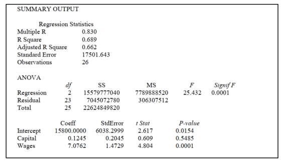
Referring to Scenario 14-5, which of the independent variables in the model are significant at the 5% level?
A) Capital, Wages
B) Capital
C) Wages
D) None of the above
سؤال
SCENARIO 14-4
A real estate builder wishes to determine how house size (House) is influenced by family income
(Income) and family size (Size). House size is measured in hundreds of square feet and income is
measured in thousands of dollars. The builder randomly selected 50 families and ran the multiple
regression. Partial Microsoft Excel output is provided below:
Referring to Scenario 14-4, at the 0.01 level of significance, what conclusion should the builder reach regarding the inclusion of Income in the regression model?
A) Income is significant in explaining house size and should be included in the model because its p-value is less than 0.01.
B) Income is significant in explaining house size and should be included in the model because its p-value is more than 0.01.
C) Income is not significant in explaining house size and should not be included in the model because its p-value is less than 0.01.
D) Income is not significant in explaining house size and should not be included in the model because its p-value is more than 0.01.
سؤال
SCENARIO 14-5
A microeconomist wants to determine how corporate sales are influenced by capital and wage
spending by companies. She proceeds to randomly select 26 large corporations and record
information in millions of dollars. The Microsoft Excel output below shows results of this multiple
regression.
Referring to Scenario 14-5, what is the p-value for testing whether Wages have a positive impact on corporate sales?
A) 0.01
B) 0.05
C) 0.0001
D) 0.00005
سؤال
SCENARIO 14-4
A real estate builder wishes to determine how house size (House) is influenced by family income
(Income) and family size (Size). House size is measured in hundreds of square feet and income is
measured in thousands of dollars. The builder randomly selected 50 families and ran the multiple
regression. Partial Microsoft Excel output is provided below:
Referring to Scenario 14-4, the partial F test for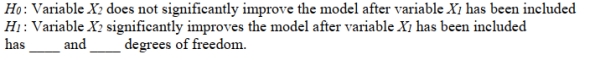 .
.
A real estate builder wishes to determine how house size (House) is influenced by family income
(Income) and family size (Size). House size is measured in hundreds of square feet and income is
measured in thousands of dollars. The builder randomly selected 50 families and ran the multiple
regression. Partial Microsoft Excel output is provided below:
Referring to Scenario 14-4, the partial F test for
. سؤال
SCENARIO 14-4
A real estate builder wishes to determine how house size (House) is influenced by family income
(Income) and family size (Size). House size is measured in hundreds of square feet and income is
measured in thousands of dollars. The builder randomly selected 50 families and ran the multiple
regression. Partial Microsoft Excel output is provided below:
Referring to Scenario 14-4, the coefficient of partial determination ⋅ is ____.
A real estate builder wishes to determine how house size (House) is influenced by family income
(Income) and family size (Size). House size is measured in hundreds of square feet and income is
measured in thousands of dollars. The builder randomly selected 50 families and ran the multiple
regression. Partial Microsoft Excel output is provided below:
Referring to Scenario 14-4, the coefficient of partial determination
⋅ is ____. سؤال
SCENARIO 14-4
A real estate builder wishes to determine how house size (House) is influenced by family income
(Income) and family size (Size). House size is measured in hundreds of square feet and income is
measured in thousands of dollars. The builder randomly selected 50 families and ran the multiple
regression. Partial Microsoft Excel output is provided below:
Referring to Scenario 14-4, ____% of the variation in the house size can be explained by the
variation in the family size while holding the family income constant.
سؤال
SCENARIO 14-5
A microeconomist wants to determine how corporate sales are influenced by capital and wage
spending by companies. She proceeds to randomly select 26 large corporations and record
information in millions of dollars. The Microsoft Excel output below shows results of this multiple
regression.
Referring to Scenario 14-5, what fraction of the variability in sales is explained by spending on capital and wages?
A) 27.0%
B) 50.9%
C) 68.9%
D) 83.0%
سؤال
SCENARIO 14-4
A real estate builder wishes to determine how house size (House) is influenced by family income
(Income) and family size (Size). House size is measured in hundreds of square feet and income is
measured in thousands of dollars. The builder randomly selected 50 families and ran the multiple
regression. Partial Microsoft Excel output is provided below:
Referring to Scenario 14-4, at the 0.01 level of significance, what conclusion should the builder draw regarding the inclusion of Size in the regression model?
A) Size is significant in explaining house size and should be included in the model because its p-value is less than 0.01.
B) Size is significant in explaining house size and should be included in the model because its p-value is more than 0.01.
C) Size is not significant in explaining house size and should not be included in the model because its p-value is less than 0.01.
D) Size is not significant in explaining house size and should not be included in the model because its p-value is more than 0.01.
سؤال
SCENARIO 14-4
A real estate builder wishes to determine how house size (House) is influenced by family income
(Income) and family size (Size). House size is measured in hundreds of square feet and income is
measured in thousands of dollars. The builder randomly selected 50 families and ran the multiple
regression. Partial Microsoft Excel output is provided below:
Referring to Scenario 14-4, the partial F test for
H0 : Variable X1 does not significantly improve the model after variable X2 has been included
H1 : Variable X1 significantly improves the model after variable X2 has been included
has ____ and ____ degrees of freedom.
سؤال
SCENARIO 14-4
A real estate builder wishes to determine how house size (House) is influenced by family income
(Income) and family size (Size). House size is measured in hundreds of square feet and income is
measured in thousands of dollars. The builder randomly selected 50 families and ran the multiple
regression. Partial Microsoft Excel output is provided below:
Referring to Scenario 14-4, the value of the partial F test statistic is ____ for
سؤال
SCENARIO 14-5
A microeconomist wants to determine how corporate sales are influenced by capital and wage
spending by companies. She proceeds to randomly select 26 large corporations and record
information in millions of dollars. The Microsoft Excel output below shows results of this multiple
regression.
Referring to Scenario 14-5, when the microeconomist used a simple linear regression model with sales as the dependent variable and wages as the independent variable, she obtained an r2 value of
0)601. What additional percentage of the total variation of sales has been explained by including
Capital spending in the multiple regression?
A) 60.1%
B) 31.1%
C) 22.9%
D) 8.8%
سؤال
SCENARIO 14-4
A real estate builder wishes to determine how house size (House) is influenced by family income
(Income) and family size (Size). House size is measured in hundreds of square feet and income is
measured in thousands of dollars. The builder randomly selected 50 families and ran the multiple
regression. Partial Microsoft Excel output is provided below:
Referring to Scenario 14-4, the observed value of the F-statistic is missing from the printout. What are the degrees of freedom for this F-statistic?
A) 2 for the numerator, 47 for the denominator
B) 2 for the numerator, 49 for the denominator
C) 49 for the numerator, 47 for the denominator
D) 47 for the numerator, 49 for the denominator
سؤال
SCENARIO 14-4
A real estate builder wishes to determine how house size (House) is influenced by family income
(Income) and family size (Size). House size is measured in hundreds of square feet and income is
measured in thousands of dollars. The builder randomly selected 50 families and ran the multiple
regression. Partial Microsoft Excel output is provided below:
Referring to Scenario 14-4, ____% of the variation in the house size can be explained by the
variation in the family income while holding the family size constant.
سؤال
SCENARIO 14-5
A microeconomist wants to determine how corporate sales are influenced by capital and wage
spending by companies. She proceeds to randomly select 26 large corporations and record
information in millions of dollars. The Microsoft Excel output below shows results of this multiple
regression.
Referring to Scenario 14-5, what is the p-value for Wages?
A) 0.01
B) 0.05
C) 0.0001
D) None of the above
سؤال
SCENARIO 14-4
A real estate builder wishes to determine how house size (House) is influenced by family income
(Income) and family size (Size). House size is measured in hundreds of square feet and income is
measured in thousands of dollars. The builder randomly selected 50 families and ran the multiple
regression. Partial Microsoft Excel output is provided below:
Referring to Scenario 14-4, what is the value of the calculated F test statistic that is missing from
the output for testing whether the whole regression model is significant?
سؤال
SCENARIO 14-4
A real estate builder wishes to determine how house size (House) is influenced by family income
(Income) and family size (Size). House size is measured in hundreds of square feet and income is
measured in thousands of dollars. The builder randomly selected 50 families and ran the multiple
regression. Partial Microsoft Excel output is provided below:
Referring to Scenario 14-4, what are the regression degrees of freedom that are missing from the output?
A) 2
B) 47
C) 49
D) 50
سؤال
SCENARIO 14-4
A real estate builder wishes to determine how house size (House) is influenced by family income
(Income) and family size (Size). House size is measured in hundreds of square feet and income is
measured in thousands of dollars. The builder randomly selected 50 families and ran the multiple
regression. Partial Microsoft Excel output is provided below:
Referring to Scenario 14-4, what are the residual degrees of freedom that are missing from the output?
A) 2
B) 47
C) 49
D) 50
سؤال
SCENARIO 14-4
A real estate builder wishes to determine how house size (House) is influenced by family income
(Income) and family size (Size). House size is measured in hundreds of square feet and income is
measured in thousands of dollars. The builder randomly selected 50 families and ran the multiple
regression. Partial Microsoft Excel output is provided below:
Referring to Scenario 14-4, suppose the builder wants to test whether the coefficient on Size is significantly different from 0. What is the value of the relevant t-statistic?
A) -0.7630
B) 3.2708
C) 10.8668
D) 60.0864
سؤال
SCENARIO 14-4
A real estate builder wishes to determine how house size (House) is influenced by family income
(Income) and family size (Size). House size is measured in hundreds of square feet and income is
measured in thousands of dollars. The builder randomly selected 50 families and ran the multiple
regression. Partial Microsoft Excel output is provided below:
Referring to Scenario 14-4, the coefficient of partial determination rY221⋅ is ____.
سؤال
SCENARIO 14-4
A real estate builder wishes to determine how house size (House) is influenced by family income
(Income) and family size (Size). House size is measured in hundreds of square feet and income is
measured in thousands of dollars. The builder randomly selected 50 families and ran the multiple
regression. Partial Microsoft Excel output is provided below:
Referring to Scenario 14-4, the value of the partial F test statistic is ____ for
سؤال
SCENARIO 14-5
A microeconomist wants to determine how corporate sales are influenced by capital and wage
spending by companies. She proceeds to randomly select 26 large corporations and record
information in millions of dollars. The Microsoft Excel output below shows results of this multiple
regression.
Referring to Scenario 14-5, what are the predicted sales (in millions of dollars) for a company spending $100 million on capital and $100 million on wages?
A) 15,800.00
B) 16,520.07
C) 17,277.49
D) 20,455.98
سؤال
14-22 Introduction to Multiple Regression 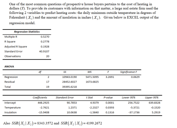
Referring to Scenario 14-6, the partial F test for
Referring to Scenario 14-6, the partial F test for
سؤال
14-22 Introduction to Multiple Regression One of the most common questions of prospective house buyers pertains to the cost of heating in dollars . To provide its customers with information on that matter, a large real estate firm used the following 2 variables to predict heating costs: the daily minimum outside temperature in degrees of Fahrenheit and the amount of insulation in inches . Given below is EXCEL output of the regression model.
ANOVA
![<strong>14-22 Introduction to Multiple Regression One of the most common questions of prospective house buyers pertains to the cost of heating in dollars ( Y ) . To provide its customers with information on that matter, a large real estate firm used the following 2 variables to predict heating costs: the daily minimum outside temperature in degrees of Fahrenheit \left( X _ { 1 } \right) and the amount of insulation in inches \left( X _ { 2 } \right) . Given below is EXCEL output of the regression model. \begin{array}{lr} \hline {\text { Regression Statistics }} \\ \hline \text { Multiple R } & 0.5270 \\ \text { R Square } & 0.2778 \\ \text { Adjusted R Square } & 0.1928 \\ \text { Standard Error } & 40.9107 \\ \text { Observations } & 20 \\ \hline \end{array} ANOVA \begin{array}{lrrrrrr} & \text { Coefficients } & \text { Standard Error } & t \text { Stat } & \text { P-value } & \text { Lower 95\% } & \text { Upper 95\% } \\ \hline \text { Intercept } & 448.2925 & 90.7853 & 4.9379 & 0.0001 & 256.7522 & 639.8328 \\ \text { Temperature } & -2.7621 & 1.2371 & -2.2327 & 0.0393 & -5.3721 & -0.1520 \\ \text { Insulation } & -15.9408 & 10.0638 & -1.5840 & 0.1316 & -37.1736 \end{array} Also \operatorname { SSR } \left( X _ { 1 } \mid X _ { 2 } \right) = 8343.3572 and \operatorname { SSR } \left( X _ { 2 } \mid X _ { 1 } \right) = 4199.2672 -Referring to Scenario 14-6, what is the 95% confidence interval for the expected change in heating costs as a result of a 1 degree Fahrenheit change in the daily minimum outside Temperature?</strong> A) [256.7522, 639.8328] B) [204.7854, 497.1733] C) [?5.3721, ?0.1520] D) [?37.1736, 5.2919] <div style=padding-top: 35px>](https://d2lvgg3v3hfg70.cloudfront.net/TB4636/11ee035f_cd00_01bf_a563_d51adb884ebb_TB4636_11.jpg)
Also and
-Referring to Scenario 14-6, what is the 95% confidence interval for the expected change in heating costs as a result of a 1 degree Fahrenheit change in the daily minimum outside
Temperature?
A) [256.7522, 639.8328]
B) [204.7854, 497.1733]
C) [?5.3721, ?0.1520]
D) [?37.1736, 5.2919]
ANOVA
Also and
-Referring to Scenario 14-6, what is the 95% confidence interval for the expected change in heating costs as a result of a 1 degree Fahrenheit change in the daily minimum outside
Temperature?
A) [256.7522, 639.8328]
B) [204.7854, 497.1733]
C) [?5.3721, ?0.1520]
D) [?37.1736, 5.2919]
سؤال
14-22 Introduction to Multiple Regression
Referring to Scenario 14-6, the coefficient of partial determination ⋅ is ____.
Referring to Scenario 14-6, the coefficient of partial determination
⋅ is ____. سؤال
14-22 Introduction to Multiple Regression One of the most common questions of prospective house buyers pertains to the cost of heating in dollars . To provide its customers with information on that matter, a large real estate firm used the following 2 variables to predict heating costs: the daily minimum outside temperature in degrees of Fahrenheit and the amount of insulation in inches . Given below is EXCEL output of the regression model.
ANOVA
Also and
-Referring to Scenario 14-6, the estimated value of the regression parameter in means that
A) holding the effect of the amount of insulation constant, an estimated expected $1 increase in heating costs is associated with a decrease in the daily minimum outside temperature
By 2.76 degrees.
B) holding the effect of the amount of insulation constant, a 1 degree increase in the daily minimum outside temperature results in a decrease in heating costs by $2.76.
C) holding the effect of the amount of insulation constant, a 1 degree increase in the daily minimum outside temperature results in an estimated decrease in mean heating costs by
$2)76.
D) holding the effect of the amount of insulation constant, a 1% increase in the daily minimum outside temperature results in an estimated decrease in mean heating costs by
2)76%.
سؤال
SCENARIO 14-5
A microeconomist wants to determine how corporate sales are influenced by capital and wage
spending by companies. She proceeds to randomly select 26 large corporations and record
information in millions of dollars. The Microsoft Excel output below shows results of this multiple
regression.
Referring to Scenario 14-5, suppose the microeconomist wants to test whether the coefficient on Capital is significantly different from 0. What is the value of the relevant t-statistic?
A) 0.609
B) 2.617
C) 4.804
D) 25.432
سؤال
SCENARIO 14-5
A microeconomist wants to determine how corporate sales are influenced by capital and wage
spending by companies. She proceeds to randomly select 26 large corporations and record
information in millions of dollars. The Microsoft Excel output below shows results of this multiple
regression.
Referring to Scenario 14-5, at the 0.01 level of significance, what conclusion should the microeconomist reach regarding the inclusion of Capital in the regression model?
A) Capital is significant in explaining corporate sales and should be included in the model because its p-value is less than 0.01.
B) Capital is significant in explaining corporate sales and should be included in the model because its p-value is more than 0.01.
C) Capital is not significant in explaining corporate sales and should not be included in the model because its p-value is less than 0.01.
D) Capital is not significant in explaining corporate sales and should not be included in the model because its p-value is more than 0.01.
سؤال
14-22 Introduction to Multiple Regression One of the most common questions of prospective house buyers pertains to the cost of heating in dollars . To provide its customers with information on that matter, a large real estate firm used the following 2 variables to predict heating costs: the daily minimum outside temperature in degrees of Fahrenheit and the amount of insulation in inches . Given below is EXCEL output of the regression model.
ANOVA
Also and
-Referring to Scenario 14-6, what can we say about the regression model?
A) The model explains 17.12% of the variability of heating costs; after correcting for the degrees of freedom, the model explains 27.78% of the sample variability of heating costs.
B) The model explains 19.28% of the variability of heating costs; after correcting for the degrees of freedom, the model explains 27.78% of the sample variability of heating costs.
C) The model explains 27.78% of the variability of heating costs; after correcting for the degrees of freedom, the model explains 19.28% of the sample variability of heating costs.
D) The model explains 19.28% of the variability of heating costs; after correcting for the degrees of freedom, the model explains 17.12% of the sample variability of heating costs.
سؤال
SCENARIO 14-5
A microeconomist wants to determine how corporate sales are influenced by capital and wage
spending by companies. She proceeds to randomly select 26 large corporations and record
information in millions of dollars. The Microsoft Excel output below shows results of this multiple
regression.
Referring to Scenario 14-5, what is the p-value for testing whether Capital has a negative influence on corporate sales?
A) 0.05
B) 0.2743
C) 0.5485
D) 0.7258
سؤال
SCENARIO 14-5
A microeconomist wants to determine how corporate sales are influenced by capital and wage
spending by companies. She proceeds to randomly select 26 large corporations and record
information in millions of dollars. The Microsoft Excel output below shows results of this multiple
regression.
Referring to Scenario 14-5, one company in the sample had sales of $21.439 billion (Sales = 21,439). This company spent $300 million on capital and $700 million on wages. What is the
Residual (in millions of dollars) for this data point?
A) 790.69
B) 648.31
C) -648.31
D) -790.69
سؤال
SCENARIO 14-5
A microeconomist wants to determine how corporate sales are influenced by capital and wage
spending by companies. She proceeds to randomly select 26 large corporations and record
information in millions of dollars. The Microsoft Excel output below shows results of this multiple
regression.
Referring to Scenario 14-5, what is the p-value for testing whether Wages have a negative impact on corporate sales?
A) 0.05
B) 0.0001
C) 0.00005
D) 0.99995
سؤال
14-22 Introduction to Multiple Regression
Referring to Scenario 14-6, the value of the partial F test statistic is ____ for
Referring to Scenario 14-6, the value of the partial F test statistic is ____ for
سؤال
SCENARIO 14-5
A microeconomist wants to determine how corporate sales are influenced by capital and wage
spending by companies. She proceeds to randomly select 26 large corporations and record
information in millions of dollars. The Microsoft Excel output below shows results of this multiple
regression.
Referring to Scenario 14-5, what are the predicted sales (in millions of dollars) for a company spending $500 million on capital and $200 million on wages?
A) 15,800.00
B) 16,520.07
C) 17,277.49
D) 20,455.98
سؤال
14-22 Introduction to Multiple Regression
Referring to Scenario 14-6, the value of the partial F test statistic is ____ for
Referring to Scenario 14-6, the value of the partial F test statistic is ____ for
سؤال
SCENARIO 14-5
A microeconomist wants to determine how corporate sales are influenced by capital and wage
spending by companies. She proceeds to randomly select 26 large corporations and record
information in millions of dollars. The Microsoft Excel output below shows results of this multiple
regression.
Referring to Scenario 14-5, the observed value of the F-statistic is given on the printout as 25.432. What are the degrees of freedom for this F-statistic?
A) 25 for the numerator, 2 for the denominator
B) 2 for the numerator, 23 for the denominator
C) 23 for the numerator, 25 for the denominator
D) 2 for the numerator, 25 for the denominator
سؤال
SCENARIO 14-5
A microeconomist wants to determine how corporate sales are influenced by capital and wage
spending by companies. She proceeds to randomly select 26 large corporations and record
information in millions of dollars. The Microsoft Excel output below shows results of this multiple
regression.
Referring to Scenario 14-5, one company in the sample had sales of $20 billion (Sales = 20,000). This company spent $300 million on capital and $700 million on wages. What is the residual (in
Millions of dollars) for this data point?
A) 874.55
B) 622.87
C) -790.69
D) -983.56
سؤال
14-22 Introduction to Multiple Regression
Referring to Scenario 14-6, the partial F test for
Referring to Scenario 14-6, the partial F test for
سؤال
SCENARIO 14-5
A microeconomist wants to determine how corporate sales are influenced by capital and wage
spending by companies. She proceeds to randomly select 26 large corporations and record
information in millions of dollars. The Microsoft Excel output below shows results of this multiple
regression.
Referring to Scenario 14-5, what is the p-value for Capital?
A) 0.01
B) 0.025
C) 0.05
D) None of the above
سؤال
SCENARIO 14-5
A microeconomist wants to determine how corporate sales are influenced by capital and wage
spending by companies. She proceeds to randomly select 26 large corporations and record
information in millions of dollars. The Microsoft Excel output below shows results of this multiple
regression.
Referring to Scenario 14-5, what is the p-value for testing whether Capital has a positive influence on corporate sales?
A) 0.025
B) 0.05
C) 0.2743
D) 0.5485
سؤال
SCENARIO 14-5
A microeconomist wants to determine how corporate sales are influenced by capital and wage
spending by companies. She proceeds to randomly select 26 large corporations and record
information in millions of dollars. The Microsoft Excel output below shows results of this multiple
regression.
Referring to Scenario 14-5, which of the following values for α is the smallest for which the regression model as a whole is significant?
A) 0.00005
B) 0.001
C) 0.01
D) 0.05

فتح الحزمة
قم بالتسجيل لفتح البطاقات في هذه المجموعة!
Unlock Deck
Unlock Deck
1/394
العب
ملء الشاشة (f)
Deck 14: Introduction to Multiple
1
SCENARIO 14-3
An economist is interested to see how consumption for an economy (in $ billions) is influenced by
gross domestic product ($ billions) and aggregate price (consumer price index). The Microsoft Excel
output of this regression is partially reproduced below.
Referring to Scenario 14-3, what is the estimated mean consumption level for an economy with GDP equal to $2 billion and an aggregate price index of 90?
A) $1.39 billion
B) $2.89 billion
C) $4.75 billion
D) $9.45 billion
A
2
SCENARIO 14-1 A manager of a product sales group believes the number of sales made by an employee depends on how many years that employee has been with the company and how he/she scored on a business aptitude test . A random sample of 8 employees provides the following:
-Referring to Scenario 14-1, if an employee who had been with the company 5 years scored a 9 on the aptitude test, what would his estimated expected sales be?
A) 79.09
B) 60.88
C) 55.62
D) 17.98
-Referring to Scenario 14-1, if an employee who had been with the company 5 years scored a 9 on the aptitude test, what would his estimated expected sales be?
A) 79.09
B) 60.88
C) 55.62
D) 17.98
79.09
3
SCENARIO 14-2 A professor of industrial relations believes that an individual's wage rate at a factory depends on his performance rating and the number of economics courses the employee successfully completed in college . The professor randomly selects 6 workers and collects the following information:
-Referring to Scenario 14-2, an employee who took 12 economics courses scores 10 on the performance rating. What is her estimated expected wage rate?
A) 10.90
B) 12.20
C) 24.87
D) 25.70
-Referring to Scenario 14-2, an employee who took 12 economics courses scores 10 on the performance rating. What is her estimated expected wage rate?
A) 10.90
B) 12.20
C) 24.87
D) 25.70
24.87
4
SCENARIO 14-2 A professor of industrial relations believes that an individual's wage rate at a factory depends on his performance rating and the number of economics courses the employee successfully completed in college . The professor randomly selects 6 workers and collects the following information:
-Referring to Scenario 14-2, for these data, what is the value for the regression constant, b0?
A) 0.616
B) 1.054
C) 6.932
D) 9.103
-Referring to Scenario 14-2, for these data, what is the value for the regression constant, b0?
A) 0.616
B) 1.054
C) 6.932
D) 9.103
فتح الحزمة
افتح القفل للوصول البطاقات البالغ عددها 394 في هذه المجموعة.
فتح الحزمة
k this deck
5
In a multiple regression model, the value of the coefficient of multiple determination
فتح الحزمة
افتح القفل للوصول البطاقات البالغ عددها 394 في هذه المجموعة.
فتح الحزمة
k this deck
6
SCENARIO 14-3
An economist is interested to see how consumption for an economy (in $ billions) is influenced by
gross domestic product ($ billions) and aggregate price (consumer price index). The Microsoft Excel
output of this regression is partially reproduced below.
Referring to Scenario 14-3, the p-value for GDP is
A) 0.05
B) 0.01
C) 0.001
D) None of the above.
فتح الحزمة
افتح القفل للوصول البطاقات البالغ عددها 394 في هذه المجموعة.
فتح الحزمة
k this deck
7
SCENARIO 14-2 A professor of industrial relations believes that an individual's wage rate at a factory depends on his performance rating and the number of economics courses the employee successfully completed in college . The professor randomly selects 6 workers and collects the following information:
-Referring to Scenario 14-2, for these data, what is the estimated coefficient for the number of economics courses taken, ?
A) 0.616
B) 1.054
C) 6.932
D) 9.103
-Referring to Scenario 14-2, for these data, what is the estimated coefficient for the number of economics courses taken, ?
A) 0.616
B) 1.054
C) 6.932
D) 9.103
فتح الحزمة
افتح القفل للوصول البطاقات البالغ عددها 394 في هذه المجموعة.
فتح الحزمة
k this deck
8
SCENARIO 14-3
An economist is interested to see how consumption for an economy (in $ billions) is influenced by
gross domestic product ($ billions) and aggregate price (consumer price index). The Microsoft Excel
output of this regression is partially reproduced below.
-Referring to Scenario 14-3, when the economist used a simple linear regression model with consumption as the dependent variable and GDP as the independent variable, he obtained an value of 0.971. What additional percentage of the total variation of consumption has been
Explained by including aggregate prices in the multiple regression?
A) 98.2
B) 11.1
C) 2.8
D) 1.1
فتح الحزمة
افتح القفل للوصول البطاقات البالغ عددها 394 في هذه المجموعة.
فتح الحزمة
k this deck
9
SCENARIO 14-1 A manager of a product sales group believes the number of sales made by an employee depends on how many years that employee has been with the company and how he/she scored on a business aptitude test . A random sample of 8 employees provides the following:
-Referring to Scenario 14-1, for these data, what is the value for the regression constant, b0?
A) 0.998
B) 3.103
C) 4.698
D) 21.293
-Referring to Scenario 14-1, for these data, what is the value for the regression constant, b0?
A) 0.998
B) 3.103
C) 4.698
D) 21.293
فتح الحزمة
افتح القفل للوصول البطاقات البالغ عددها 394 في هذه المجموعة.
فتح الحزمة
k this deck
10
SCENARIO 14-3
An economist is interested to see how consumption for an economy (in $ billions) is influenced by
gross domestic product ($ billions) and aggregate price (consumer price index). The Microsoft Excel
output of this regression is partially reproduced below.
Referring to Scenario 14-3, what is the predicted consumption level for an economy with GDP equal to $4 billion and an aggregate price index of 150?
A) $1.39 billion
B) $2.89 billion
C) $4.75 billion
D) $9.45 billion
فتح الحزمة
افتح القفل للوصول البطاقات البالغ عددها 394 في هذه المجموعة.
فتح الحزمة
k this deck
11
In a multiple regression model, which of the following is correct regarding the value of the adjusted r2 ?
A) It can be negative.
B) It has to be positive.
C) It has to be larger than the coefficient of multiple determination.
D) It can be larger than 1.
A) It can be negative.
B) It has to be positive.
C) It has to be larger than the coefficient of multiple determination.
D) It can be larger than 1.
فتح الحزمة
افتح القفل للوصول البطاقات البالغ عددها 394 في هذه المجموعة.
فتح الحزمة
k this deck
12
SCENARIO 14-3
An economist is interested to see how consumption for an economy (in $ billions) is influenced by
gross domestic product ($ billions) and aggregate price (consumer price index). The Microsoft Excel
output of this regression is partially reproduced below.
Referring to Scenario 14-3, the p-value for the regression model as a whole is
A) 0.05
B) 0.01
C) 0.001
D) None of the above.
فتح الحزمة
افتح القفل للوصول البطاقات البالغ عددها 394 في هذه المجموعة.
فتح الحزمة
k this deck
13
SCENARIO 14-2 A professor of industrial relations believes that an individual's wage rate at a factory depends on his performance rating and the number of economics courses the employee successfully completed in college . The professor randomly selects 6 workers and collects the following information:
-Referring to Scenario 14-2, suppose an employee had never taken an economics course and managed to score a 5 on his performance rating. What is his estimated expected wage rate?
A) 10.90
B) 12.20
C) 17.23
D) 25.11
-Referring to Scenario 14-2, suppose an employee had never taken an economics course and managed to score a 5 on his performance rating. What is his estimated expected wage rate?
A) 10.90
B) 12.20
C) 17.23
D) 25.11
فتح الحزمة
افتح القفل للوصول البطاقات البالغ عددها 394 في هذه المجموعة.
فتح الحزمة
k this deck
14
SCENARIO 14-1 A manager of a product sales group believes the number of sales made by an employee depends on how many years that employee has been with the company and how he/she scored on a business aptitude test . A random sample of 8 employees provides the following:
-Referring to Scenario 14-1, for these data, what is the estimated coefficient for the variable representing years an employee has been with the company, b1?
A) 0.998
B) 3.103
C) 4.698
D) 21.293
-Referring to Scenario 14-1, for these data, what is the estimated coefficient for the variable representing years an employee has been with the company, b1?
A) 0.998
B) 3.103
C) 4.698
D) 21.293
فتح الحزمة
افتح القفل للوصول البطاقات البالغ عددها 394 في هذه المجموعة.
فتح الحزمة
k this deck
15
SCENARIO 14-2 A professor of industrial relations believes that an individual's wage rate at a factory depends on his performance rating and the number of economics courses the employee successfully completed in college . The professor randomly selects 6 workers and collects the following information:
-Referring to Scenario 14-2, for these data, what is the estimated coefficient for performance rating, b1?
A) 0.616
B) 1.054
C) 6.932
D) 9.103
-Referring to Scenario 14-2, for these data, what is the estimated coefficient for performance rating, b1?
A) 0.616
B) 1.054
C) 6.932
D) 9.103
فتح الحزمة
افتح القفل للوصول البطاقات البالغ عددها 394 في هذه المجموعة.
فتح الحزمة
k this deck
16
SCENARIO 14-3
An economist is interested to see how consumption for an economy (in $ billions) is influenced by
gross domestic product ($ billions) and aggregate price (consumer price index). The Microsoft Excel
output of this regression is partially reproduced below.
Referring to Scenario 14-3, the p-value for the aggregated price index is
A) 0.05
B) 0.01
C) 0.001
D) None of the above.
فتح الحزمة
افتح القفل للوصول البطاقات البالغ عددها 394 في هذه المجموعة.
فتح الحزمة
k this deck
17
SCENARIO 14-1 A manager of a product sales group believes the number of sales made by an employee depends on how many years that employee has been with the company and how he/she scored on a business aptitude test . A random sample of 8 employees provides the following:
-Referring to Scenario 14-1, for these data, what is the estimated coefficient for the variable representing scores on the aptitude test, b2?
A) 0.998
B) 3.103
C) 4.698
D) 21.293
-Referring to Scenario 14-1, for these data, what is the estimated coefficient for the variable representing scores on the aptitude test, b2?
A) 0.998
B) 3.103
C) 4.698
D) 21.293
فتح الحزمة
افتح القفل للوصول البطاقات البالغ عددها 394 في هذه المجموعة.
فتح الحزمة
k this deck
18
SCENARIO 14-2 A professor of industrial relations believes that an individual's wage rate at a factory depends on his performance rating and the number of economics courses the employee successfully completed in college . The professor randomly selects 6 workers and collects the following information:
-The variation attributable to factors other than the relationship between the independent variables and the explained variable in a regression analysis is represented by
A) regression sum of squares.
B) error sum of squares.
C) total sum of squares.
D) regression mean squares.
-The variation attributable to factors other than the relationship between the independent variables and the explained variable in a regression analysis is represented by
A) regression sum of squares.
B) error sum of squares.
C) total sum of squares.
D) regression mean squares.
فتح الحزمة
افتح القفل للوصول البطاقات البالغ عددها 394 في هذه المجموعة.
فتح الحزمة
k this deck
19
SCENARIO 14-3
An economist is interested to see how consumption for an economy (in $ billions) is influenced by
gross domestic product ($ billions) and aggregate price (consumer price index). The Microsoft Excel
output of this regression is partially reproduced below.
Referring to Scenario 14-3, one economy in the sample had an aggregate consumption level of $3 billion, a GDP of $3.5 billion, and an aggregate price level of 125. What is the residual for this
Data point?
A) $2.52 billion
B) $0.48 billion
C) - $1.33 billion
D) - $2.52 billion
فتح الحزمة
افتح القفل للوصول البطاقات البالغ عددها 394 في هذه المجموعة.
فتح الحزمة
k this deck
20
SCENARIO 14-3
An economist is interested to see how consumption for an economy (in $ billions) is influenced by
gross domestic product ($ billions) and aggregate price (consumer price index). The Microsoft Excel
output of this regression is partially reproduced below.
Referring to Scenario 14-3, what is the estimated mean consumption level for an economy with GDP equal to $4 billion and an aggregate price index of 150?
A) $1.39 billion
B) $2.89 billion
C) $4.75 billion
D) $9.45 billion
فتح الحزمة
افتح القفل للوصول البطاقات البالغ عددها 394 في هذه المجموعة.
فتح الحزمة
k this deck
21
SCENARIO 14-4
A real estate builder wishes to determine how house size (House) is influenced by family income
(Income) and family size (Size). House size is measured in hundreds of square feet and income is
measured in thousands of dollars. The builder randomly selected 50 families and ran the multiple
regression. Partial Microsoft Excel output is provided below:
Referring to Scenario 14-4, suppose the builder wants to test whether the coefficient on Income is significantly different from 0. What is the value of the relevant t-statistic?
A) -0.7630
B) 3.2708
C) 10.8668
D) 60.0864
فتح الحزمة
افتح القفل للوصول البطاقات البالغ عددها 394 في هذه المجموعة.
فتح الحزمة
k this deck
22
SCENARIO 14-4
A real estate builder wishes to determine how house size (House) is influenced by family income
(Income) and family size (Size). House size is measured in hundreds of square feet and income is
measured in thousands of dollars. The builder randomly selected 50 families and ran the multiple
regression. Partial Microsoft Excel output is provided below:
Referring to Scenario 14-4, what is the predicted house size (in hundreds of square feet) for an
individual earning an annual income of $40,000 and having a family size of 4?
فتح الحزمة
افتح القفل للوصول البطاقات البالغ عددها 394 في هذه المجموعة.
فتح الحزمة
k this deck
23
SCENARIO 14-4
A real estate builder wishes to determine how house size (House) is influenced by family income
(Income) and family size (Size). House size is measured in hundreds of square feet and income is
measured in thousands of dollars. The builder randomly selected 50 families and ran the multiple
regression. Partial Microsoft Excel output is provided below:
Referring to Scenario 14-4, what fraction of the variability in house size is explained by income and size of family?
A) 17.56%
B) 70.69%
C) 71.89%
D) 84.79%
فتح الحزمة
افتح القفل للوصول البطاقات البالغ عددها 394 في هذه المجموعة.
فتح الحزمة
k this deck
24
SCENARIO 14-4
A real estate builder wishes to determine how house size (House) is influenced by family income
(Income) and family size (Size). House size is measured in hundreds of square feet and income is
measured in thousands of dollars. The builder randomly selected 50 families and ran the multiple
regression. Partial Microsoft Excel output is provided below:
Referring to Scenario 14-4, one individual in the sample had an annual income of $40,000 and a
family size of 1. This individual owned a home with an area of 1,000 square feet (House =
10.00). What is the residual (in hundreds of square feet) for this data point?
فتح الحزمة
افتح القفل للوصول البطاقات البالغ عددها 394 في هذه المجموعة.
فتح الحزمة
k this deck
25
SCENARIO 14-3
An economist is interested to see how consumption for an economy (in $ billions) is influenced by
gross domestic product ($ billions) and aggregate price (consumer price index). The Microsoft Excel
output of this regression is partially reproduced below.
Referring to Scenario 14-3, to test for the significance of the coefficient on gross domestic product, the p-value is
A) 0.0001
B) 0.8330
C) 0.8837
D) 0.9999
فتح الحزمة
افتح القفل للوصول البطاقات البالغ عددها 394 في هذه المجموعة.
فتح الحزمة
k this deck
26
SCENARIO 14-4
A real estate builder wishes to determine how house size (House) is influenced by family income
(Income) and family size (Size). House size is measured in hundreds of square feet and income is
measured in thousands of dollars. The builder randomly selected 50 families and ran the multiple
regression. Partial Microsoft Excel output is provided below:
Referring to Scenario 14-4, which of the following values for the level of significance is the smallest for which at least one explanatory variable is significant individually?
A) 0.005
B) 0.010
C) 0.025
D) 0.050
فتح الحزمة
افتح القفل للوصول البطاقات البالغ عددها 394 في هذه المجموعة.
فتح الحزمة
k this deck
27
SCENARIO 14-4
A real estate builder wishes to determine how house size (House) is influenced by family income
(Income) and family size (Size). House size is measured in hundreds of square feet and income is
measured in thousands of dollars. The builder randomly selected 50 families and ran the multiple
regression. Partial Microsoft Excel output is provided below:
-Referring to Scenario 14-4, when the builder used a simple linear regression model with house size (House) as the dependent variable and family size (Size) as the independent variable, he
Obtained an value of 1.25%. What additional percentage of the total variation in house size has
Been explained by including income in the multiple regression?
A) 15.00%
B) 70.64%
C) 71.50%
D) 73.62%
فتح الحزمة
افتح القفل للوصول البطاقات البالغ عددها 394 في هذه المجموعة.
فتح الحزمة
k this deck
28
SCENARIO 14-3
An economist is interested to see how consumption for an economy (in $ billions) is influenced by
gross domestic product ($ billions) and aggregate price (consumer price index). The Microsoft Excel
output of this regression is partially reproduced below.
Referring to Scenario 14-3, to test whether aggregate price index has a positive impact on consumption, the p-value is
A) 0.0001
B) 0.4165
C) 0.5835
D) 0.8330
فتح الحزمة
افتح القفل للوصول البطاقات البالغ عددها 394 في هذه المجموعة.
فتح الحزمة
k this deck
29
SCENARIO 14-4
A real estate builder wishes to determine how house size (House) is influenced by family income
(Income) and family size (Size). House size is measured in hundreds of square feet and income is
measured in thousands of dollars. The builder randomly selected 50 families and ran the multiple
regression. Partial Microsoft Excel output is provided below:
Referring to Scenario 14-4, what annual income (in thousands of dollars) would an individual
with a family size of 9 need to attain a predicted 5,000 square foot home (House = 50)?
فتح الحزمة
افتح القفل للوصول البطاقات البالغ عددها 394 في هذه المجموعة.
فتح الحزمة
k this deck
30
SCENARIO 14-4
A real estate builder wishes to determine how house size (House) is influenced by family income
(Income) and family size (Size). House size is measured in hundreds of square feet and income is
measured in thousands of dollars. The builder randomly selected 50 families and ran the multiple
regression. Partial Microsoft Excel output is provided below:
Referring to Scenario 14-4, which of the following values for the level of significance is the smallest for which each explanatory variable is significant individually?
A) 0.001
B) 0.010
C) 0.025
D) 0.050
فتح الحزمة
افتح القفل للوصول البطاقات البالغ عددها 394 في هذه المجموعة.
فتح الحزمة
k this deck
31
SCENARIO 14-4
A real estate builder wishes to determine how house size (House) is influenced by family income
(Income) and family size (Size). House size is measured in hundreds of square feet and income is
measured in thousands of dollars. The builder randomly selected 50 families and ran the multiple
regression. Partial Microsoft Excel output is provided below:
Referring to Scenario 14-4, what annual income (in thousands of dollars) would an individual
with a family size of 4 need to attain a predicted 10,000 square foot home (House = 100)?
فتح الحزمة
افتح القفل للوصول البطاقات البالغ عددها 394 في هذه المجموعة.
فتح الحزمة
k this deck
32
SCENARIO 14-3
An economist is interested to see how consumption for an economy (in $ billions) is influenced by
gross domestic product ($ billions) and aggregate price (consumer price index). The Microsoft Excel
output of this regression is partially reproduced below.
Referring to Scenario 14-3, one economy in the sample had an aggregate consumption level of $4 billion, a GDP of $6 billion, and an aggregate price level of 200. What is the residual for this data
Point?
A) $4.39 billion
B) $0.39 billion
C) - $0.39 billion
D) - $1.33 billion
فتح الحزمة
افتح القفل للوصول البطاقات البالغ عددها 394 في هذه المجموعة.
فتح الحزمة
k this deck
33
SCENARIO 14-4
A real estate builder wishes to determine how house size (House) is influenced by family income
(Income) and family size (Size). House size is measured in hundreds of square feet and income is
measured in thousands of dollars. The builder randomly selected 50 families and ran the multiple
regression. Partial Microsoft Excel output is provided below:
Referring to Scenario 14-4, one individual in the sample had an annual income of $100,000 and a
family size of 10. This individual owned a home with an area of 7,000 square feet (House =
70.00). What is the residual (in hundreds of square feet) for this data point?
فتح الحزمة
افتح القفل للوصول البطاقات البالغ عددها 394 في هذه المجموعة.
فتح الحزمة
k this deck
34
SCENARIO 14-4
A real estate builder wishes to determine how house size (House) is influenced by family income
(Income) and family size (Size). House size is measured in hundreds of square feet and income is
measured in thousands of dollars. The builder randomly selected 50 families and ran the multiple
regression. Partial Microsoft Excel output is provided below:
Referring to Scenario 14-4, which of the following values for the level of significance is the smallest for which at most one explanatory variable is significant individually?
A) 0.001
B) 0.010
C) 0.025
D) 0.050
فتح الحزمة
افتح القفل للوصول البطاقات البالغ عددها 394 في هذه المجموعة.
فتح الحزمة
k this deck
35
SCENARIO 14-4
A real estate builder wishes to determine how house size (House) is influenced by family income
(Income) and family size (Size). House size is measured in hundreds of square feet and income is
measured in thousands of dollars. The builder randomly selected 50 families and ran the multiple
regression. Partial Microsoft Excel output is provided below:
Referring to Scenario 14-4, which of the independent variables in the model are significant at the 5% level?
A) Income only
B) Size only
C) Income and Size
D) None
فتح الحزمة
افتح القفل للوصول البطاقات البالغ عددها 394 في هذه المجموعة.
فتح الحزمة
k this deck
36
SCENARIO 14-3
An economist is interested to see how consumption for an economy (in $ billions) is influenced by
gross domestic product ($ billions) and aggregate price (consumer price index). The Microsoft Excel
output of this regression is partially reproduced below.
Referring to Scenario 14-3, to test for the significance of the coefficient on aggregate price index, the value of the relevant t-statistic is
A) 2.365
B) 0.143
C) - 0.219
D) - 1.960
فتح الحزمة
افتح القفل للوصول البطاقات البالغ عددها 394 في هذه المجموعة.
فتح الحزمة
k this deck
37
SCENARIO 14-3
An economist is interested to see how consumption for an economy (in $ billions) is influenced by
gross domestic product ($ billions) and aggregate price (consumer price index). The Microsoft Excel
output of this regression is partially reproduced below.
Referring to Scenario 14-3, to test for the significance of the coefficient on aggregate price index, the p-value is
A) 0.0001
B) 0.8330
C) 0.8837
D) 0.9999
فتح الحزمة
افتح القفل للوصول البطاقات البالغ عددها 394 في هذه المجموعة.
فتح الحزمة
k this deck
38
SCENARIO 14-3
An economist is interested to see how consumption for an economy (in $ billions) is influenced by
gross domestic product ($ billions) and aggregate price (consumer price index). The Microsoft Excel
output of this regression is partially reproduced below.
Referring to Scenario 14-3, to test whether aggregate price index has a negative impact on consumption, the p-value is _______?
A) 0.0001
B) 0.4165
C) 0.8330
D) 0.8837
فتح الحزمة
افتح القفل للوصول البطاقات البالغ عددها 394 في هذه المجموعة.
فتح الحزمة
k this deck
39
SCENARIO 14-4
A real estate builder wishes to determine how house size (House) is influenced by family income
(Income) and family size (Size). House size is measured in hundreds of square feet and income is
measured in thousands of dollars. The builder randomly selected 50 families and ran the multiple
regression. Partial Microsoft Excel output is provided below:
Referring to Scenario 14-4, which of the following values for the level of significance is the smallest for which the regression model as a whole is significant?
A) 0.0005
B) 0.001
C) 0.01
D) 0.05
فتح الحزمة
افتح القفل للوصول البطاقات البالغ عددها 394 في هذه المجموعة.
فتح الحزمة
k this deck
40
SCENARIO 14-3
An economist is interested to see how consumption for an economy (in $ billions) is influenced by
gross domestic product ($ billions) and aggregate price (consumer price index). The Microsoft Excel
output of this regression is partially reproduced below.
Referring to Scenario 14-3, to test whether gross domestic product has a positive impact on consumption, the p-value is
A) 0.00005
B) 0.0001
C) 0.9999
D) 0.99995
فتح الحزمة
افتح القفل للوصول البطاقات البالغ عددها 394 في هذه المجموعة.
فتح الحزمة
k this deck
41
SCENARIO 14-5
A microeconomist wants to determine how corporate sales are influenced by capital and wage
spending by companies. She proceeds to randomly select 26 large corporations and record
information in millions of dollars. The Microsoft Excel output below shows results of this multiple
regression.
Referring to Scenario 14-5, which of the independent variables in the model are significant at the 5% level?
A) Capital, Wages
B) Capital
C) Wages
D) None of the above
فتح الحزمة
افتح القفل للوصول البطاقات البالغ عددها 394 في هذه المجموعة.
فتح الحزمة
k this deck
42
SCENARIO 14-4
A real estate builder wishes to determine how house size (House) is influenced by family income
(Income) and family size (Size). House size is measured in hundreds of square feet and income is
measured in thousands of dollars. The builder randomly selected 50 families and ran the multiple
regression. Partial Microsoft Excel output is provided below:
Referring to Scenario 14-4, at the 0.01 level of significance, what conclusion should the builder reach regarding the inclusion of Income in the regression model?
A) Income is significant in explaining house size and should be included in the model because its p-value is less than 0.01.
B) Income is significant in explaining house size and should be included in the model because its p-value is more than 0.01.
C) Income is not significant in explaining house size and should not be included in the model because its p-value is less than 0.01.
D) Income is not significant in explaining house size and should not be included in the model because its p-value is more than 0.01.
فتح الحزمة
افتح القفل للوصول البطاقات البالغ عددها 394 في هذه المجموعة.
فتح الحزمة
k this deck
43
SCENARIO 14-5
A microeconomist wants to determine how corporate sales are influenced by capital and wage
spending by companies. She proceeds to randomly select 26 large corporations and record
information in millions of dollars. The Microsoft Excel output below shows results of this multiple
regression.
Referring to Scenario 14-5, what is the p-value for testing whether Wages have a positive impact on corporate sales?
A) 0.01
B) 0.05
C) 0.0001
D) 0.00005
فتح الحزمة
افتح القفل للوصول البطاقات البالغ عددها 394 في هذه المجموعة.
فتح الحزمة
k this deck
44
SCENARIO 14-4
A real estate builder wishes to determine how house size (House) is influenced by family income
(Income) and family size (Size). House size is measured in hundreds of square feet and income is
measured in thousands of dollars. The builder randomly selected 50 families and ran the multiple
regression. Partial Microsoft Excel output is provided below:
Referring to Scenario 14-4, the partial F test for .
A real estate builder wishes to determine how house size (House) is influenced by family income
(Income) and family size (Size). House size is measured in hundreds of square feet and income is
measured in thousands of dollars. The builder randomly selected 50 families and ran the multiple
regression. Partial Microsoft Excel output is provided below:
Referring to Scenario 14-4, the partial F test for
. فتح الحزمة
افتح القفل للوصول البطاقات البالغ عددها 394 في هذه المجموعة.
فتح الحزمة
k this deck
45
SCENARIO 14-4
A real estate builder wishes to determine how house size (House) is influenced by family income
(Income) and family size (Size). House size is measured in hundreds of square feet and income is
measured in thousands of dollars. The builder randomly selected 50 families and ran the multiple
regression. Partial Microsoft Excel output is provided below:
Referring to Scenario 14-4, the coefficient of partial determination ⋅ is ____.
A real estate builder wishes to determine how house size (House) is influenced by family income
(Income) and family size (Size). House size is measured in hundreds of square feet and income is
measured in thousands of dollars. The builder randomly selected 50 families and ran the multiple
regression. Partial Microsoft Excel output is provided below:
Referring to Scenario 14-4, the coefficient of partial determination
⋅ is ____. فتح الحزمة
افتح القفل للوصول البطاقات البالغ عددها 394 في هذه المجموعة.
فتح الحزمة
k this deck
46
SCENARIO 14-4
A real estate builder wishes to determine how house size (House) is influenced by family income
(Income) and family size (Size). House size is measured in hundreds of square feet and income is
measured in thousands of dollars. The builder randomly selected 50 families and ran the multiple
regression. Partial Microsoft Excel output is provided below:
Referring to Scenario 14-4, ____% of the variation in the house size can be explained by the
variation in the family size while holding the family income constant.
فتح الحزمة
افتح القفل للوصول البطاقات البالغ عددها 394 في هذه المجموعة.
فتح الحزمة
k this deck
47
SCENARIO 14-5
A microeconomist wants to determine how corporate sales are influenced by capital and wage
spending by companies. She proceeds to randomly select 26 large corporations and record
information in millions of dollars. The Microsoft Excel output below shows results of this multiple
regression.
Referring to Scenario 14-5, what fraction of the variability in sales is explained by spending on capital and wages?
A) 27.0%
B) 50.9%
C) 68.9%
D) 83.0%
فتح الحزمة
افتح القفل للوصول البطاقات البالغ عددها 394 في هذه المجموعة.
فتح الحزمة
k this deck
48
SCENARIO 14-4
A real estate builder wishes to determine how house size (House) is influenced by family income
(Income) and family size (Size). House size is measured in hundreds of square feet and income is
measured in thousands of dollars. The builder randomly selected 50 families and ran the multiple
regression. Partial Microsoft Excel output is provided below:
Referring to Scenario 14-4, at the 0.01 level of significance, what conclusion should the builder draw regarding the inclusion of Size in the regression model?
A) Size is significant in explaining house size and should be included in the model because its p-value is less than 0.01.
B) Size is significant in explaining house size and should be included in the model because its p-value is more than 0.01.
C) Size is not significant in explaining house size and should not be included in the model because its p-value is less than 0.01.
D) Size is not significant in explaining house size and should not be included in the model because its p-value is more than 0.01.
فتح الحزمة
افتح القفل للوصول البطاقات البالغ عددها 394 في هذه المجموعة.
فتح الحزمة
k this deck
49
SCENARIO 14-4
A real estate builder wishes to determine how house size (House) is influenced by family income
(Income) and family size (Size). House size is measured in hundreds of square feet and income is
measured in thousands of dollars. The builder randomly selected 50 families and ran the multiple
regression. Partial Microsoft Excel output is provided below:
Referring to Scenario 14-4, the partial F test for
H0 : Variable X1 does not significantly improve the model after variable X2 has been included
H1 : Variable X1 significantly improves the model after variable X2 has been included
has ____ and ____ degrees of freedom.
فتح الحزمة
افتح القفل للوصول البطاقات البالغ عددها 394 في هذه المجموعة.
فتح الحزمة
k this deck
50
SCENARIO 14-4
A real estate builder wishes to determine how house size (House) is influenced by family income
(Income) and family size (Size). House size is measured in hundreds of square feet and income is
measured in thousands of dollars. The builder randomly selected 50 families and ran the multiple
regression. Partial Microsoft Excel output is provided below:
Referring to Scenario 14-4, the value of the partial F test statistic is ____ for
فتح الحزمة
افتح القفل للوصول البطاقات البالغ عددها 394 في هذه المجموعة.
فتح الحزمة
k this deck
51
SCENARIO 14-5
A microeconomist wants to determine how corporate sales are influenced by capital and wage
spending by companies. She proceeds to randomly select 26 large corporations and record
information in millions of dollars. The Microsoft Excel output below shows results of this multiple
regression.
Referring to Scenario 14-5, when the microeconomist used a simple linear regression model with sales as the dependent variable and wages as the independent variable, she obtained an r2 value of
0)601. What additional percentage of the total variation of sales has been explained by including
Capital spending in the multiple regression?
A) 60.1%
B) 31.1%
C) 22.9%
D) 8.8%
فتح الحزمة
افتح القفل للوصول البطاقات البالغ عددها 394 في هذه المجموعة.
فتح الحزمة
k this deck
52
SCENARIO 14-4
A real estate builder wishes to determine how house size (House) is influenced by family income
(Income) and family size (Size). House size is measured in hundreds of square feet and income is
measured in thousands of dollars. The builder randomly selected 50 families and ran the multiple
regression. Partial Microsoft Excel output is provided below:
Referring to Scenario 14-4, the observed value of the F-statistic is missing from the printout. What are the degrees of freedom for this F-statistic?
A) 2 for the numerator, 47 for the denominator
B) 2 for the numerator, 49 for the denominator
C) 49 for the numerator, 47 for the denominator
D) 47 for the numerator, 49 for the denominator
فتح الحزمة
افتح القفل للوصول البطاقات البالغ عددها 394 في هذه المجموعة.
فتح الحزمة
k this deck
53
SCENARIO 14-4
A real estate builder wishes to determine how house size (House) is influenced by family income
(Income) and family size (Size). House size is measured in hundreds of square feet and income is
measured in thousands of dollars. The builder randomly selected 50 families and ran the multiple
regression. Partial Microsoft Excel output is provided below:
Referring to Scenario 14-4, ____% of the variation in the house size can be explained by the
variation in the family income while holding the family size constant.
فتح الحزمة
افتح القفل للوصول البطاقات البالغ عددها 394 في هذه المجموعة.
فتح الحزمة
k this deck
54
SCENARIO 14-5
A microeconomist wants to determine how corporate sales are influenced by capital and wage
spending by companies. She proceeds to randomly select 26 large corporations and record
information in millions of dollars. The Microsoft Excel output below shows results of this multiple
regression.
Referring to Scenario 14-5, what is the p-value for Wages?
A) 0.01
B) 0.05
C) 0.0001
D) None of the above
فتح الحزمة
افتح القفل للوصول البطاقات البالغ عددها 394 في هذه المجموعة.
فتح الحزمة
k this deck
55
SCENARIO 14-4
A real estate builder wishes to determine how house size (House) is influenced by family income
(Income) and family size (Size). House size is measured in hundreds of square feet and income is
measured in thousands of dollars. The builder randomly selected 50 families and ran the multiple
regression. Partial Microsoft Excel output is provided below:
Referring to Scenario 14-4, what is the value of the calculated F test statistic that is missing from
the output for testing whether the whole regression model is significant?
فتح الحزمة
افتح القفل للوصول البطاقات البالغ عددها 394 في هذه المجموعة.
فتح الحزمة
k this deck
56
SCENARIO 14-4
A real estate builder wishes to determine how house size (House) is influenced by family income
(Income) and family size (Size). House size is measured in hundreds of square feet and income is
measured in thousands of dollars. The builder randomly selected 50 families and ran the multiple
regression. Partial Microsoft Excel output is provided below:
Referring to Scenario 14-4, what are the regression degrees of freedom that are missing from the output?
A) 2
B) 47
C) 49
D) 50
فتح الحزمة
افتح القفل للوصول البطاقات البالغ عددها 394 في هذه المجموعة.
فتح الحزمة
k this deck
57
SCENARIO 14-4
A real estate builder wishes to determine how house size (House) is influenced by family income
(Income) and family size (Size). House size is measured in hundreds of square feet and income is
measured in thousands of dollars. The builder randomly selected 50 families and ran the multiple
regression. Partial Microsoft Excel output is provided below:
Referring to Scenario 14-4, what are the residual degrees of freedom that are missing from the output?
A) 2
B) 47
C) 49
D) 50
فتح الحزمة
افتح القفل للوصول البطاقات البالغ عددها 394 في هذه المجموعة.
فتح الحزمة
k this deck
58
SCENARIO 14-4
A real estate builder wishes to determine how house size (House) is influenced by family income
(Income) and family size (Size). House size is measured in hundreds of square feet and income is
measured in thousands of dollars. The builder randomly selected 50 families and ran the multiple
regression. Partial Microsoft Excel output is provided below:
Referring to Scenario 14-4, suppose the builder wants to test whether the coefficient on Size is significantly different from 0. What is the value of the relevant t-statistic?
A) -0.7630
B) 3.2708
C) 10.8668
D) 60.0864
فتح الحزمة
افتح القفل للوصول البطاقات البالغ عددها 394 في هذه المجموعة.
فتح الحزمة
k this deck
59
SCENARIO 14-4
A real estate builder wishes to determine how house size (House) is influenced by family income
(Income) and family size (Size). House size is measured in hundreds of square feet and income is
measured in thousands of dollars. The builder randomly selected 50 families and ran the multiple
regression. Partial Microsoft Excel output is provided below:
Referring to Scenario 14-4, the coefficient of partial determination rY221⋅ is ____.
فتح الحزمة
افتح القفل للوصول البطاقات البالغ عددها 394 في هذه المجموعة.
فتح الحزمة
k this deck
60
SCENARIO 14-4
A real estate builder wishes to determine how house size (House) is influenced by family income
(Income) and family size (Size). House size is measured in hundreds of square feet and income is
measured in thousands of dollars. The builder randomly selected 50 families and ran the multiple
regression. Partial Microsoft Excel output is provided below:
Referring to Scenario 14-4, the value of the partial F test statistic is ____ for
فتح الحزمة
افتح القفل للوصول البطاقات البالغ عددها 394 في هذه المجموعة.
فتح الحزمة
k this deck
61
SCENARIO 14-5
A microeconomist wants to determine how corporate sales are influenced by capital and wage
spending by companies. She proceeds to randomly select 26 large corporations and record
information in millions of dollars. The Microsoft Excel output below shows results of this multiple
regression.
Referring to Scenario 14-5, what are the predicted sales (in millions of dollars) for a company spending $100 million on capital and $100 million on wages?
A) 15,800.00
B) 16,520.07
C) 17,277.49
D) 20,455.98
فتح الحزمة
افتح القفل للوصول البطاقات البالغ عددها 394 في هذه المجموعة.
فتح الحزمة
k this deck
62
14-22 Introduction to Multiple Regression
Referring to Scenario 14-6, the partial F test for
Referring to Scenario 14-6, the partial F test for
فتح الحزمة
افتح القفل للوصول البطاقات البالغ عددها 394 في هذه المجموعة.
فتح الحزمة
k this deck
63
14-22 Introduction to Multiple Regression One of the most common questions of prospective house buyers pertains to the cost of heating in dollars . To provide its customers with information on that matter, a large real estate firm used the following 2 variables to predict heating costs: the daily minimum outside temperature in degrees of Fahrenheit and the amount of insulation in inches . Given below is EXCEL output of the regression model.
ANOVA
Also and
-Referring to Scenario 14-6, what is the 95% confidence interval for the expected change in heating costs as a result of a 1 degree Fahrenheit change in the daily minimum outside
Temperature?
A) [256.7522, 639.8328]
B) [204.7854, 497.1733]
C) [?5.3721, ?0.1520]
D) [?37.1736, 5.2919]
ANOVA
Also and
-Referring to Scenario 14-6, what is the 95% confidence interval for the expected change in heating costs as a result of a 1 degree Fahrenheit change in the daily minimum outside
Temperature?
A) [256.7522, 639.8328]
B) [204.7854, 497.1733]
C) [?5.3721, ?0.1520]
D) [?37.1736, 5.2919]
فتح الحزمة
افتح القفل للوصول البطاقات البالغ عددها 394 في هذه المجموعة.
فتح الحزمة
k this deck
64
14-22 Introduction to Multiple Regression
Referring to Scenario 14-6, the coefficient of partial determination ⋅ is ____.
Referring to Scenario 14-6, the coefficient of partial determination
⋅ is ____. فتح الحزمة
افتح القفل للوصول البطاقات البالغ عددها 394 في هذه المجموعة.
فتح الحزمة
k this deck
65
14-22 Introduction to Multiple Regression One of the most common questions of prospective house buyers pertains to the cost of heating in dollars . To provide its customers with information on that matter, a large real estate firm used the following 2 variables to predict heating costs: the daily minimum outside temperature in degrees of Fahrenheit and the amount of insulation in inches . Given below is EXCEL output of the regression model.
ANOVA
Also and
-Referring to Scenario 14-6, the estimated value of the regression parameter in means that
A) holding the effect of the amount of insulation constant, an estimated expected $1 increase in heating costs is associated with a decrease in the daily minimum outside temperature
By 2.76 degrees.
B) holding the effect of the amount of insulation constant, a 1 degree increase in the daily minimum outside temperature results in a decrease in heating costs by $2.76.
C) holding the effect of the amount of insulation constant, a 1 degree increase in the daily minimum outside temperature results in an estimated decrease in mean heating costs by
$2)76.
D) holding the effect of the amount of insulation constant, a 1% increase in the daily minimum outside temperature results in an estimated decrease in mean heating costs by
2)76%.
فتح الحزمة
افتح القفل للوصول البطاقات البالغ عددها 394 في هذه المجموعة.
فتح الحزمة
k this deck
66
SCENARIO 14-5
A microeconomist wants to determine how corporate sales are influenced by capital and wage
spending by companies. She proceeds to randomly select 26 large corporations and record
information in millions of dollars. The Microsoft Excel output below shows results of this multiple
regression.
Referring to Scenario 14-5, suppose the microeconomist wants to test whether the coefficient on Capital is significantly different from 0. What is the value of the relevant t-statistic?
A) 0.609
B) 2.617
C) 4.804
D) 25.432
فتح الحزمة
افتح القفل للوصول البطاقات البالغ عددها 394 في هذه المجموعة.
فتح الحزمة
k this deck
67
SCENARIO 14-5
A microeconomist wants to determine how corporate sales are influenced by capital and wage
spending by companies. She proceeds to randomly select 26 large corporations and record
information in millions of dollars. The Microsoft Excel output below shows results of this multiple
regression.
Referring to Scenario 14-5, at the 0.01 level of significance, what conclusion should the microeconomist reach regarding the inclusion of Capital in the regression model?
A) Capital is significant in explaining corporate sales and should be included in the model because its p-value is less than 0.01.
B) Capital is significant in explaining corporate sales and should be included in the model because its p-value is more than 0.01.
C) Capital is not significant in explaining corporate sales and should not be included in the model because its p-value is less than 0.01.
D) Capital is not significant in explaining corporate sales and should not be included in the model because its p-value is more than 0.01.
فتح الحزمة
افتح القفل للوصول البطاقات البالغ عددها 394 في هذه المجموعة.
فتح الحزمة
k this deck
68
14-22 Introduction to Multiple Regression One of the most common questions of prospective house buyers pertains to the cost of heating in dollars . To provide its customers with information on that matter, a large real estate firm used the following 2 variables to predict heating costs: the daily minimum outside temperature in degrees of Fahrenheit and the amount of insulation in inches . Given below is EXCEL output of the regression model.
ANOVA
Also and
-Referring to Scenario 14-6, what can we say about the regression model?
A) The model explains 17.12% of the variability of heating costs; after correcting for the degrees of freedom, the model explains 27.78% of the sample variability of heating costs.
B) The model explains 19.28% of the variability of heating costs; after correcting for the degrees of freedom, the model explains 27.78% of the sample variability of heating costs.
C) The model explains 27.78% of the variability of heating costs; after correcting for the degrees of freedom, the model explains 19.28% of the sample variability of heating costs.
D) The model explains 19.28% of the variability of heating costs; after correcting for the degrees of freedom, the model explains 17.12% of the sample variability of heating costs.
فتح الحزمة
افتح القفل للوصول البطاقات البالغ عددها 394 في هذه المجموعة.
فتح الحزمة
k this deck
69
SCENARIO 14-5
A microeconomist wants to determine how corporate sales are influenced by capital and wage
spending by companies. She proceeds to randomly select 26 large corporations and record
information in millions of dollars. The Microsoft Excel output below shows results of this multiple
regression.
Referring to Scenario 14-5, what is the p-value for testing whether Capital has a negative influence on corporate sales?
A) 0.05
B) 0.2743
C) 0.5485
D) 0.7258
فتح الحزمة
افتح القفل للوصول البطاقات البالغ عددها 394 في هذه المجموعة.
فتح الحزمة
k this deck
70
SCENARIO 14-5
A microeconomist wants to determine how corporate sales are influenced by capital and wage
spending by companies. She proceeds to randomly select 26 large corporations and record
information in millions of dollars. The Microsoft Excel output below shows results of this multiple
regression.
Referring to Scenario 14-5, one company in the sample had sales of $21.439 billion (Sales = 21,439). This company spent $300 million on capital and $700 million on wages. What is the
Residual (in millions of dollars) for this data point?
A) 790.69
B) 648.31
C) -648.31
D) -790.69
فتح الحزمة
افتح القفل للوصول البطاقات البالغ عددها 394 في هذه المجموعة.
فتح الحزمة
k this deck
71
SCENARIO 14-5
A microeconomist wants to determine how corporate sales are influenced by capital and wage
spending by companies. She proceeds to randomly select 26 large corporations and record
information in millions of dollars. The Microsoft Excel output below shows results of this multiple
regression.
Referring to Scenario 14-5, what is the p-value for testing whether Wages have a negative impact on corporate sales?
A) 0.05
B) 0.0001
C) 0.00005
D) 0.99995
فتح الحزمة
افتح القفل للوصول البطاقات البالغ عددها 394 في هذه المجموعة.
فتح الحزمة
k this deck
72
14-22 Introduction to Multiple Regression
Referring to Scenario 14-6, the value of the partial F test statistic is ____ for
Referring to Scenario 14-6, the value of the partial F test statistic is ____ for
فتح الحزمة
افتح القفل للوصول البطاقات البالغ عددها 394 في هذه المجموعة.
فتح الحزمة
k this deck
73
SCENARIO 14-5
A microeconomist wants to determine how corporate sales are influenced by capital and wage
spending by companies. She proceeds to randomly select 26 large corporations and record
information in millions of dollars. The Microsoft Excel output below shows results of this multiple
regression.
Referring to Scenario 14-5, what are the predicted sales (in millions of dollars) for a company spending $500 million on capital and $200 million on wages?
A) 15,800.00
B) 16,520.07
C) 17,277.49
D) 20,455.98
فتح الحزمة
افتح القفل للوصول البطاقات البالغ عددها 394 في هذه المجموعة.
فتح الحزمة
k this deck
74
14-22 Introduction to Multiple Regression
Referring to Scenario 14-6, the value of the partial F test statistic is ____ for
Referring to Scenario 14-6, the value of the partial F test statistic is ____ for
فتح الحزمة
افتح القفل للوصول البطاقات البالغ عددها 394 في هذه المجموعة.
فتح الحزمة
k this deck
75
SCENARIO 14-5
A microeconomist wants to determine how corporate sales are influenced by capital and wage
spending by companies. She proceeds to randomly select 26 large corporations and record
information in millions of dollars. The Microsoft Excel output below shows results of this multiple
regression.
Referring to Scenario 14-5, the observed value of the F-statistic is given on the printout as 25.432. What are the degrees of freedom for this F-statistic?
A) 25 for the numerator, 2 for the denominator
B) 2 for the numerator, 23 for the denominator
C) 23 for the numerator, 25 for the denominator
D) 2 for the numerator, 25 for the denominator
فتح الحزمة
افتح القفل للوصول البطاقات البالغ عددها 394 في هذه المجموعة.
فتح الحزمة
k this deck
76
SCENARIO 14-5
A microeconomist wants to determine how corporate sales are influenced by capital and wage
spending by companies. She proceeds to randomly select 26 large corporations and record
information in millions of dollars. The Microsoft Excel output below shows results of this multiple
regression.
Referring to Scenario 14-5, one company in the sample had sales of $20 billion (Sales = 20,000). This company spent $300 million on capital and $700 million on wages. What is the residual (in
Millions of dollars) for this data point?
A) 874.55
B) 622.87
C) -790.69
D) -983.56
فتح الحزمة
افتح القفل للوصول البطاقات البالغ عددها 394 في هذه المجموعة.
فتح الحزمة
k this deck
77
14-22 Introduction to Multiple Regression
Referring to Scenario 14-6, the partial F test for
Referring to Scenario 14-6, the partial F test for
فتح الحزمة
افتح القفل للوصول البطاقات البالغ عددها 394 في هذه المجموعة.
فتح الحزمة
k this deck
78
SCENARIO 14-5
A microeconomist wants to determine how corporate sales are influenced by capital and wage
spending by companies. She proceeds to randomly select 26 large corporations and record
information in millions of dollars. The Microsoft Excel output below shows results of this multiple
regression.
Referring to Scenario 14-5, what is the p-value for Capital?
A) 0.01
B) 0.025
C) 0.05
D) None of the above
فتح الحزمة
افتح القفل للوصول البطاقات البالغ عددها 394 في هذه المجموعة.
فتح الحزمة
k this deck
79
SCENARIO 14-5
A microeconomist wants to determine how corporate sales are influenced by capital and wage
spending by companies. She proceeds to randomly select 26 large corporations and record
information in millions of dollars. The Microsoft Excel output below shows results of this multiple
regression.
Referring to Scenario 14-5, what is the p-value for testing whether Capital has a positive influence on corporate sales?
A) 0.025
B) 0.05
C) 0.2743
D) 0.5485
فتح الحزمة
افتح القفل للوصول البطاقات البالغ عددها 394 في هذه المجموعة.
فتح الحزمة
k this deck
80
SCENARIO 14-5
A microeconomist wants to determine how corporate sales are influenced by capital and wage
spending by companies. She proceeds to randomly select 26 large corporations and record
information in millions of dollars. The Microsoft Excel output below shows results of this multiple
regression.
Referring to Scenario 14-5, which of the following values for α is the smallest for which the regression model as a whole is significant?
A) 0.00005
B) 0.001
C) 0.01
D) 0.05
فتح الحزمة
افتح القفل للوصول البطاقات البالغ عددها 394 في هذه المجموعة.
فتح الحزمة
k this deck
فتح الحزمة
افتح القفل للوصول البطاقات البالغ عددها 394 في هذه المجموعة.


