Deck 14: Risk-Pooling Strategies to Reduce and Hedge Uncertainty
ملء الشاشة (f)
سؤال
سؤال
سؤال
سؤال
(Burger King) Consider the following excerpts from a Wall Street Journal article on Burger King (Beatty, 1996):
Burger King intends to bring smiles to the faces of millions of parents and children this holiday season with its "Toy Story" promotion. But it has some of them up in arms because local restaurants are running out of the popular toys … Every Kids Meal sold every day of the year comes with a giveaway, a program that has been in place for about six years and has helped Grand Metropolitan PLC's Burger King increase its market share. Nearly all of Burger King's 7,000 U.S. stores are participating in the "Toy Story" promotion … Nevertheless, meeting consumer demand still remains a conundrum for the giants. That is partly because individual Burger King restaurant owners make their tricky forecasts six months before such promotions begin. "It's asking you to pull out a crystal ball and predict exactly what consumer demand is going to be," says Richard Taylor, Burger King's director of youth and family marketing. "This is simply a case of consumer demand outstripping supply." The long lead times are necessary because the toys are produced overseas to take advantage of lower costs … Burger King managers in Houston and Atlanta say the freebies are running out there, too … But Burger King, which ordered nearly 50 million of the small plastic dolls, is "nowhere near running out of toys on a national level."
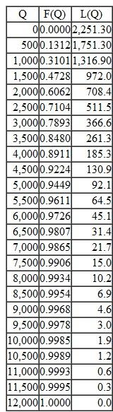
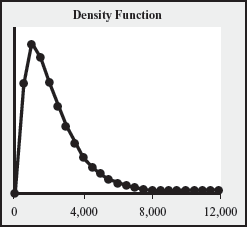
Let's consider a simplified analysis of Burger King's situation. Consider a region with 200 restaurants served by a single distribution center. At the time the order must be placed with the factories in Asia, demand (units of toys) for the promotion at each restaurant is forecasted to be gamma distributed with mean 2,251 and standard deviation 1,600. A discrete version of that gamma distribution is provided in the following table, along with a graph of the density function:
Suppose, six months in advance of the promotion, Burger King must make a single order for each restaurant. Furthermore, Burger King wants to have an in-stock probability of at least 85 percent.
a. Given those requirements, how many toys must each restaurant order
b. How many toys should Burger King expect to have at the end of the promotion Now suppose Burger King makes a single order for all 200 restaurants. The order will be delivered to the distribution center and each restaurant will receive deliveries from that stockpile as needed. If demands were independent across all restaurants, total demand would be 200 × 2,251 = 450,200 with a standard deviation of
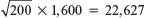 . But it is unlikely that demands will be independent across restaurants. In other words, it is likely that there is positive correlation. Nevertheless, based on historical data, Burger King estimates the coefficient of variation for the total will be half of what it is for individual stores. As a result, a normal distribution will work for the total demand forecast.
c. How many toys must Burger King order for the distribution center to have an 85 percent in-stock probability
d. If the quantity in part c is ordered, then how many units should Burger King expect to have at the end of the promotion
e. If Burger King ordered the quantity evaluated in part a (i.e., the amount such that each restaurant would have its own inventory and generate an 85 percent in-stock probability) but kept that entire quantity at the distribution center and delivered to each restaurant only as needed, then what would the DC's in-stock probability be
Burger King intends to bring smiles to the faces of millions of parents and children this holiday season with its "Toy Story" promotion. But it has some of them up in arms because local restaurants are running out of the popular toys … Every Kids Meal sold every day of the year comes with a giveaway, a program that has been in place for about six years and has helped Grand Metropolitan PLC's Burger King increase its market share. Nearly all of Burger King's 7,000 U.S. stores are participating in the "Toy Story" promotion … Nevertheless, meeting consumer demand still remains a conundrum for the giants. That is partly because individual Burger King restaurant owners make their tricky forecasts six months before such promotions begin. "It's asking you to pull out a crystal ball and predict exactly what consumer demand is going to be," says Richard Taylor, Burger King's director of youth and family marketing. "This is simply a case of consumer demand outstripping supply." The long lead times are necessary because the toys are produced overseas to take advantage of lower costs … Burger King managers in Houston and Atlanta say the freebies are running out there, too … But Burger King, which ordered nearly 50 million of the small plastic dolls, is "nowhere near running out of toys on a national level."
Let's consider a simplified analysis of Burger King's situation. Consider a region with 200 restaurants served by a single distribution center. At the time the order must be placed with the factories in Asia, demand (units of toys) for the promotion at each restaurant is forecasted to be gamma distributed with mean 2,251 and standard deviation 1,600. A discrete version of that gamma distribution is provided in the following table, along with a graph of the density function:
Suppose, six months in advance of the promotion, Burger King must make a single order for each restaurant. Furthermore, Burger King wants to have an in-stock probability of at least 85 percent.
a. Given those requirements, how many toys must each restaurant order
b. How many toys should Burger King expect to have at the end of the promotion Now suppose Burger King makes a single order for all 200 restaurants. The order will be delivered to the distribution center and each restaurant will receive deliveries from that stockpile as needed. If demands were independent across all restaurants, total demand would be 200 × 2,251 = 450,200 with a standard deviation of
. But it is unlikely that demands will be independent across restaurants. In other words, it is likely that there is positive correlation. Nevertheless, based on historical data, Burger King estimates the coefficient of variation for the total will be half of what it is for individual stores. As a result, a normal distribution will work for the total demand forecast.c. How many toys must Burger King order for the distribution center to have an 85 percent in-stock probability
d. If the quantity in part c is ordered, then how many units should Burger King expect to have at the end of the promotion
e. If Burger King ordered the quantity evaluated in part a (i.e., the amount such that each restaurant would have its own inventory and generate an 85 percent in-stock probability) but kept that entire quantity at the distribution center and delivered to each restaurant only as needed, then what would the DC's in-stock probability be
سؤال
سؤال
سؤال
سؤال
سؤال
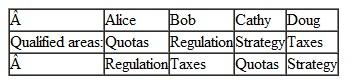
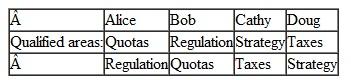
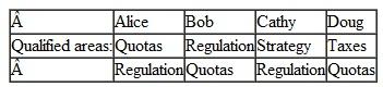
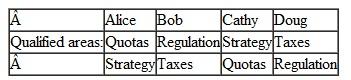
(Consulting Services) A small economic consulting firm has four employees, Alice, Bob, Cathy, and Doug. The firm offers services in four distinct areas, Quotas, Regulation, Strategy, and Taxes. At the current time Alice is qualified for Quotas, Bob does Regulation, and so on. But this isn't working too well: the firm often finds it cannot compete for business in one area because it has already committed to work in that area while in another area it is idle. Therefore, the firm would like to train the consultants to be qualified in more than one area. Which of the following assignments is likely to be most beneficial to the firm
a.
 b.
b.
 c.
c.
 d.
d.
 e.
e.

a.
b. c. d. e.
فتح الحزمة
قم بالتسجيل لفتح البطاقات في هذه المجموعة!
Unlock Deck
Unlock Deck
1/9
العب
ملء الشاشة (f)
Deck 14: Risk-Pooling Strategies to Reduce and Hedge Uncertainty
1
(Egghead) In 1997 Egghead Computers ran a chain of 50 retail stores all over the United States. Consider one type of computer sold by Egghead. Demand for this computer at each store on any given week was independently and normally distributed with a mean demand of 200 units and a standard deviation of 30 units. Inventory at each store is replenished directly from a vendor with a 10-week lead time. At the end of 1997, Egghead decided it was time to close their retail stores, put up an Internet site, and begin filling customer orders from a single warehouse.
a. By consolidating the demand into a single warehouse, what will be the resulting standard deviation of weekly demand for this computer faced by Egghead Assume Egghead's demand characteristics before and after the consolidation are identical.
b. Egghead takes physical possession of inventory when it leaves the supplier and grants possession of inventory to customers when it leaves Egghead's shipping dock. In the consolidated distribution scenario, what is the pipeline inventory
The variances of two or more independent random variables can be added up to get the overall variance. So, if there are n number of independent demand centres, the variance of a replacement consolidated centre will be the sum of variances of these independent centres. The standard deviation of the consolidated centre can off-course be found by taking the square root of its variance.
a.
Note that the standard deviation of the weekly demand in each of the single warehouses is 30.
So, the variance is
 .
.
 So, the standard deviation of the consolidated warehouse
 b.
b.
Compute the pipeline inventory as follows:
 So, there will be a pipeline inventory of

a.
Note that the standard deviation of the weekly demand in each of the single warehouses is 30.
So, the variance is
. So, the standard deviation of the consolidated warehouse b.Compute the pipeline inventory as follows:
So, there will be a pipeline inventory of 2
(Two Products) Consider two products, A and B. Demands for both products are normally distributed and have the same mean and standard deviation. The coefficient of variation of demand for each product is 0.6. The estimated correlation in demand between the two products is -0.7. What is the coefficient of variation of the total demand of the two products
The coefficient of variation (CV) of two independent random variables can be computed by knowing their individual coefficient of variation and the correlation between them. The following formula can be used.
 Where,
 are the total CV, individual CV, and correlation coefficient respectively.
Note the given information:
 Compute the coefficient of variation for total demand as follows:
 So, the coefficient of variation of total demand is

Where, are the total CV, individual CV, and correlation coefficient respectively.Note the given information:
Compute the coefficient of variation for total demand as follows: So, the coefficient of variation of total demand is 3
(Fancy Paints) Fancy Paints is a small paint store. Fancy Paints stocks 200 different SKUs (stock-keeping units) and places replenishment orders weekly. The order arrives one month (let's say four weeks) later. For the sake of simplicity, let's assume weekly demand for each SKU is Poisson distributed with mean 1.25. Fancy Paints maintains a 95 percent in-stock probability.
a. What is the average inventory at the store at the end of the week
b. Now suppose Fancy Paints purchases a color-mixing machine. This machine is expensive, but instead of stocking 200 different SKU colors, it allows Fancy Paints to stock only five basic SKUs and to obtain all the other SKUs by mixing. Weekly demand for each SKU is normally distributed with mean 50 and standard deviation 8. Suppose Fancy Paints maintains a 95 percent in-stock probability for each of the five colors. How much inventory on average is at the store at the end of the week
c. After testing the color-mixing machine for a while, the manager realizes that a 95 percent in-stock probability for each of the basic colors is not sufficient: Since mixing requires the presence of multiple mixing components, a higher in-stock probability for components is needed to maintain a 95 percent in-stock probability for the individual SKUs. The manager decides that a 98 percent in-stock probability for each of the five basic SKUs should be adequate. Suppose that each can costs $14 and 20 percent per year is charged for holding inventory (assume 50 weeks per year). What is the change in the store's holding cost relative to the original situation in which all paints are stocked individually
In a base stocking policy, the ordering is done is a fixed interval. The order-up-to level is decided based on the average demand during the lead time plus review period, its standard deviation, and the required service level percentage. The expected ending inventory at the end of the period can be computed using the following formula:
 Where
Where
 stand for the replenishment lead time and review period respectively.
a.
Note the given data:
Average weekly demand, d = 1.25
Review period, p = 1 week
Delivery lead time,
 days
days
Compute the total average ending inventory using the following method:
The in-stock probability is 0.95.
From the Poisson table, F (11) = 0.975 and F (10) = 0.946. So, the appropriate order-up-to level,
 Form the Poisson distribution table, for L (11) = 0.0467. This is the expected backorder level.
 For 200 SKUs, the total inventory level is
 b.
b.
Note the given data:
Average weekly demand, d = 50
Standard deviation of weekly demand,
 Review period, p = 1 week
Delivery lead time,
 days
days
Compute the total average ending inventory using the following method:
The required in-stock probability is 95%.
The corresponding value of
 The corresponding value of loss function is
 So, the expected back-order level


 For 5 SKUs, the total inventory level is
 c.
c.
Compare the inventory holding cost before and after the improvement in fill rate as follows:
For the in-stock probability of 98%, the corresponding value of
 The corresponding value of loss function is
 So, the expected back-order level


 For 5 SKUs, the total inventory level is
 The holding cost becomes equal to
 The holding cost with initial condition was
 So, the change in store's holding cost to the original situation is
 .
.
So, the change in store's holding cost to the original situation is

Where stand for the replenishment lead time and review period respectively.a.
Note the given data:
Average weekly demand, d = 1.25
Review period, p = 1 week
Delivery lead time,
daysCompute the total average ending inventory using the following method:
The in-stock probability is 0.95.
From the Poisson table, F (11) = 0.975 and F (10) = 0.946. So, the appropriate order-up-to level,
Form the Poisson distribution table, for L (11) = 0.0467. This is the expected backorder level. For 200 SKUs, the total inventory level is b.Note the given data:
Average weekly demand, d = 50
Standard deviation of weekly demand,
Review period, p = 1 weekDelivery lead time,
daysCompute the total average ending inventory using the following method:
The required in-stock probability is 95%.
The corresponding value of
The corresponding value of loss function is So, the expected back-order level For 5 SKUs, the total inventory level is c.Compare the inventory holding cost before and after the improvement in fill rate as follows:
For the in-stock probability of 98%, the corresponding value of
The corresponding value of loss function is So, the expected back-order level For 5 SKUs, the total inventory level is The holding cost becomes equal to The holding cost with initial condition was So, the change in store's holding cost to the original situation is .So, the change in store's holding cost to the original situation is
4
(Burger King) Consider the following excerpts from a Wall Street Journal article on Burger King (Beatty, 1996):
Burger King intends to bring smiles to the faces of millions of parents and children this holiday season with its "Toy Story" promotion. But it has some of them up in arms because local restaurants are running out of the popular toys … Every Kids Meal sold every day of the year comes with a giveaway, a program that has been in place for about six years and has helped Grand Metropolitan PLC's Burger King increase its market share. Nearly all of Burger King's 7,000 U.S. stores are participating in the "Toy Story" promotion … Nevertheless, meeting consumer demand still remains a conundrum for the giants. That is partly because individual Burger King restaurant owners make their tricky forecasts six months before such promotions begin. "It's asking you to pull out a crystal ball and predict exactly what consumer demand is going to be," says Richard Taylor, Burger King's director of youth and family marketing. "This is simply a case of consumer demand outstripping supply." The long lead times are necessary because the toys are produced overseas to take advantage of lower costs … Burger King managers in Houston and Atlanta say the freebies are running out there, too … But Burger King, which ordered nearly 50 million of the small plastic dolls, is "nowhere near running out of toys on a national level."
Let's consider a simplified analysis of Burger King's situation. Consider a region with 200 restaurants served by a single distribution center. At the time the order must be placed with the factories in Asia, demand (units of toys) for the promotion at each restaurant is forecasted to be gamma distributed with mean 2,251 and standard deviation 1,600. A discrete version of that gamma distribution is provided in the following table, along with a graph of the density function:
Suppose, six months in advance of the promotion, Burger King must make a single order for each restaurant. Furthermore, Burger King wants to have an in-stock probability of at least 85 percent.
a. Given those requirements, how many toys must each restaurant order
b. How many toys should Burger King expect to have at the end of the promotion Now suppose Burger King makes a single order for all 200 restaurants. The order will be delivered to the distribution center and each restaurant will receive deliveries from that stockpile as needed. If demands were independent across all restaurants, total demand would be 200 × 2,251 = 450,200 with a standard deviation of
. But it is unlikely that demands will be independent across restaurants. In other words, it is likely that there is positive correlation. Nevertheless, based on historical data, Burger King estimates the coefficient of variation for the total will be half of what it is for individual stores. As a result, a normal distribution will work for the total demand forecast.
c. How many toys must Burger King order for the distribution center to have an 85 percent in-stock probability
d. If the quantity in part c is ordered, then how many units should Burger King expect to have at the end of the promotion
e. If Burger King ordered the quantity evaluated in part a (i.e., the amount such that each restaurant would have its own inventory and generate an 85 percent in-stock probability) but kept that entire quantity at the distribution center and delivered to each restaurant only as needed, then what would the DC's in-stock probability be
Burger King intends to bring smiles to the faces of millions of parents and children this holiday season with its "Toy Story" promotion. But it has some of them up in arms because local restaurants are running out of the popular toys … Every Kids Meal sold every day of the year comes with a giveaway, a program that has been in place for about six years and has helped Grand Metropolitan PLC's Burger King increase its market share. Nearly all of Burger King's 7,000 U.S. stores are participating in the "Toy Story" promotion … Nevertheless, meeting consumer demand still remains a conundrum for the giants. That is partly because individual Burger King restaurant owners make their tricky forecasts six months before such promotions begin. "It's asking you to pull out a crystal ball and predict exactly what consumer demand is going to be," says Richard Taylor, Burger King's director of youth and family marketing. "This is simply a case of consumer demand outstripping supply." The long lead times are necessary because the toys are produced overseas to take advantage of lower costs … Burger King managers in Houston and Atlanta say the freebies are running out there, too … But Burger King, which ordered nearly 50 million of the small plastic dolls, is "nowhere near running out of toys on a national level."
Let's consider a simplified analysis of Burger King's situation. Consider a region with 200 restaurants served by a single distribution center. At the time the order must be placed with the factories in Asia, demand (units of toys) for the promotion at each restaurant is forecasted to be gamma distributed with mean 2,251 and standard deviation 1,600. A discrete version of that gamma distribution is provided in the following table, along with a graph of the density function:
Suppose, six months in advance of the promotion, Burger King must make a single order for each restaurant. Furthermore, Burger King wants to have an in-stock probability of at least 85 percent.
a. Given those requirements, how many toys must each restaurant order
b. How many toys should Burger King expect to have at the end of the promotion Now suppose Burger King makes a single order for all 200 restaurants. The order will be delivered to the distribution center and each restaurant will receive deliveries from that stockpile as needed. If demands were independent across all restaurants, total demand would be 200 × 2,251 = 450,200 with a standard deviation of
. But it is unlikely that demands will be independent across restaurants. In other words, it is likely that there is positive correlation. Nevertheless, based on historical data, Burger King estimates the coefficient of variation for the total will be half of what it is for individual stores. As a result, a normal distribution will work for the total demand forecast.c. How many toys must Burger King order for the distribution center to have an 85 percent in-stock probability
d. If the quantity in part c is ordered, then how many units should Burger King expect to have at the end of the promotion
e. If Burger King ordered the quantity evaluated in part a (i.e., the amount such that each restaurant would have its own inventory and generate an 85 percent in-stock probability) but kept that entire quantity at the distribution center and delivered to each restaurant only as needed, then what would the DC's in-stock probability be
فتح الحزمة
افتح القفل للوصول البطاقات البالغ عددها 9 في هذه المجموعة.
فتح الحزمة
k this deck
5
(Livingston Tools) Livingston Tools, a manufacturer of battery-operated, hand-held power tools for the consumer market (such as screwdrivers and drills), has a problem. Its two biggest customers are "big box" discounters. Because these customers are fiercely price competitive, each wants exclusive products, thereby preventing consumers from making price comparisons. For example, Livingston will sell the exact same power screwdriver to each retailer, but Livingston will use packing customized to each retailer (including two different product identification numbers). Suppose weekly demand of each product to each retailer is normally distributed with mean 5,200 and standard deviation 3,800. Livingston makes production decisions on a weekly basis and has a three-week replenishment lead time. Because these two retailers are quite important to Livingston, Livingston sets a target in-stock probability of 99.9 percent.
a. Based on the order-up-to model, what is Livingston's average inventory of each of the two versions of this power screwdriver
b. Someone at Livingston suggests that Livingston stock power screwdrivers without putting them into their specialized packaging. As orders are received from the two retailers, Livingston would fulfill those orders from the same stockpile of inventory, since it doesn't take much time to actually package each tool. Interestingly, demands at the two retailers have a slight negative correlation, -0.20. By approximately how much would this new system reduce Livingston's inventory investment
فتح الحزمة
افتح القفل للوصول البطاقات البالغ عددها 9 في هذه المجموعة.
فتح الحزمة
k this deck
6
(Restoration Hardware) Consider the following excerpts from a New York Times article (Kaufman, 2000):
Despite its early promise … Restoration has had trouble becoming a mass-market player…. What went wrong High on its own buzz, the company expanded at breakneck speed, more than doubling the number of stores, to 94, in the year and a half after the stock offering … Company managers agree, for example, that Restoration's original inventory system, which called for all furniture to be kept at stores instead of at a central warehouse, was a disaster.
Let's look at one Restoration Hardware product, a leather chair. Average weekly sales of this chair in each store is Poisson with mean 1.25 units. The replenishment lead time is 12 weeks. (This question requires using Excel to create Poisson distribution and loss function tables that are not included in the appendix. See Appendix C for the procedure to evaluate a loss function table.)
a. If each store holds its own inventory, then what is the company's annual inventory turns if the company policy is to target a 99.25 percent in-stock probability
b. Suppose Restoration Hardware builds a central warehouse to serve the 94 stores. The lead time from the supplier to the central warehouse is 12 weeks. The lead time from the central warehouse to each store is one week. Suppose the warehouse operates with a 99 percent in-stock probability, but the stores maintain a 99.25 percent in-stock probability. If only inventory at the retail stores is considered, what are Restoration's annual inventory turns
فتح الحزمة
افتح القفل للوصول البطاقات البالغ عددها 9 في هذه المجموعة.
فتح الحزمة
k this deck
7
(Study Desk) You are in charge of designing a supply chain for furniture distribution. One of your products is a study desk. This desk comes in two colors: black and cherry. Weekly demand for each desk type is normal with mean 100 and standard deviation 65 (demands for the two colors are independent). The lead time from the assembly plant to the retail store is two weeks and you order inventory replenishments weekly. There is no finished goods inventory at the plant (desks are assembled to order for delivery to the store).
a. What is the expected on-hand inventory of desks at the store (black and cherry together) if you maintain a 97 percent in-stock probability for each desk color
You notice that only the top part of the desk is black or cherry; the remainder (base) is made of the standard gray metal. Hence, you suggest that the store stock black and cherry tops separately from gray bases and assemble them when demand occurs. The replenishment lead time for components is still two weeks. Furthermore, you still choose an order-up-to level for each top to generate a 97 percent in-stock probability.
b. What is the expected on-hand inventory of black tops
c. How much less inventory of gray bases do you have on average at the store with the new in-store assembly scheme relative to the original system in which desks are delivered fully assembled ( Hint: Remember that each assembled desk requires one top and one base.)
فتح الحزمة
افتح القفل للوصول البطاقات البالغ عددها 9 في هذه المجموعة.
فتح الحزمة
k this deck
8
(O'Neill) One of O'Neill's high-end wetsuits is called the Animal. Total demand for this wetsuit is normally distributed with a mean of 200 and a standard deviation of 130. In order to ensure an excellent fit, the Animal comes in 16 sizes. Furthermore, it comes in four colors, so there are actually 64 different Animal SKUs (stock-keeping units). O'Neill sells the Animal for $350 and its production cost is $269. The Animal will be redesigned this season, so at the end of the season leftover inventory will be sold off at a steep markdown. Because this is such a niche product, O'Neill expects to receive only $100 for each leftover wetsuit. Finally, to control manufacturing costs, O'Neill has a policy that at least five wetsuits of any size/color combo must be produced at a time. Total demand for the smallest size (extra small-tall) is forecasted to be Poisson with mean 2.00. Mean demand for the four colors are black = 0.90, blue = 0.50, green = 0.40, and yellow = 0.20.
a. Suppose O'Neill already has no extra small-tall Animals in stock. What is O'Neill's expected profit if it produces one batch (five units) of extra small-tall black Animals
b. Suppose O'Neill announces that it will only sell the Animal in one color, black. If O'Neill suspects this move will reduce total demand by 12.5 percent, then what now is its expected profit from the black Animal
فتح الحزمة
افتح القفل للوصول البطاقات البالغ عددها 9 في هذه المجموعة.
فتح الحزمة
k this deck
9
(Consulting Services) A small economic consulting firm has four employees, Alice, Bob, Cathy, and Doug. The firm offers services in four distinct areas, Quotas, Regulation, Strategy, and Taxes. At the current time Alice is qualified for Quotas, Bob does Regulation, and so on. But this isn't working too well: the firm often finds it cannot compete for business in one area because it has already committed to work in that area while in another area it is idle. Therefore, the firm would like to train the consultants to be qualified in more than one area. Which of the following assignments is likely to be most beneficial to the firm
a.
b.
c.
d.
e.
a.
b. c. d. e. فتح الحزمة
افتح القفل للوصول البطاقات البالغ عددها 9 في هذه المجموعة.
فتح الحزمة
k this deck
فتح الحزمة
افتح القفل للوصول البطاقات البالغ عددها 9 في هذه المجموعة.


