Deck 10: Basic Macroeconomic Relationships
ملء الشاشة (f)
سؤال
سؤال
سؤال
سؤال
سؤال
سؤال
سؤال
سؤال
سؤال
سؤال
سؤال
سؤال
سؤال
سؤال
سؤال
سؤال
سؤال
سؤال
سؤال
KEY QUESTION Suppose that the aggregate demand and supply schedules for a hypothetical economy are as shown below:
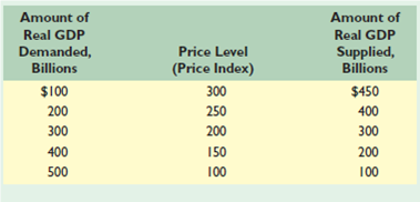
a. Use these sets of data to graph the aggregate demand and aggregate supply curves. What is the equilibrium price level and the equilibrium level of real output in this hypothetical economy Is the equilibrium real output also necessarily the full-employment real output Explain.
b. Why will a price level of 150 not be an equilibrium price level in this economy Why not 250
c. Suppose that buyers desire to purchase $200 billion of extra real output at each price level. Sketch in the new aggregate demand curve as AD 1. What factors might cause this change in aggregate demand What is the new equilibrium price level and level of real output
سؤال
Complete the accompanying table.
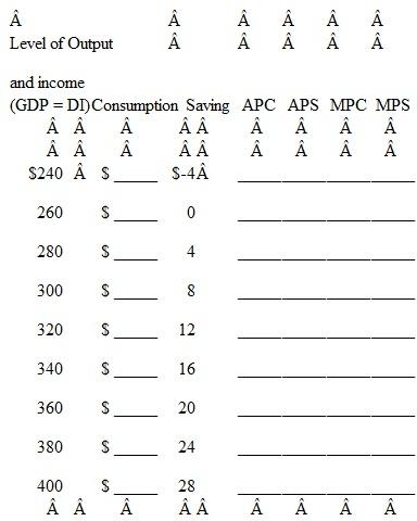
Data for completing the table (top to bottom). Consumption: $244; $260; $276; $292; $308; $324; $340; $356; $372. APC: 1.02; 1.00;.99;.97;.96;.95;.94;.94;.93. APS: -.02;.00;.01;.03;.04;.05;.06;.06;.07. MPC:.80 throughout. MPS:.20 throughout.
a. Show the consumption and saving schedules graphically.
b. Find the break even level of income. Explain how is it possible for households to dissave at very low income levels.
c. If the proportion of total income consumed (APC) decreases and the proportion saved (APS) increases as income rises, explain both verbally and graphically how the MPC and MPS can be constant at various levels of income.
سؤال

فتح الحزمة
قم بالتسجيل لفتح البطاقات في هذه المجموعة!
Unlock Deck
Unlock Deck
1/21
العب
ملء الشاشة (f)
Deck 10: Basic Macroeconomic Relationships
1
Suppose a handbill publisher can buy a new duplicating machine for $500 and the duplicator has a 1-year life. The machine is expected to contribute $550 to the year's net revenue. What is the expected rate of return If the real interest rate at which funds can be borrowed to purchase the machine is 8 percent, will the publisher choose to invest in the machine Explain.
There are two major economic functions of the interest rate. (1) Interest rates affect the level of domestic output as the monetary authorities deliberately vary them by changing the money supply. Low interest rates encourage investment, and this tends to expand the economy. High interest rates discourage investment and this tends to restrain inflation or contract the economy. (2) Interest rates allocate capital to its most productive uses. When interest rates are, say, at 10 percent, a project that expects to earn 8 percent after the payment of all costs will not be undertaken, because the cost of the borrowed money is greater than the return expected on it. This is true even if the firm is using its own money. Why make 8 percent on the project with the firm's money when lending it will earn 10 percent On the other hand, all projects that are expected to return more than the interest rate will be undertaken. The interest rate thus allocates money capital to those investments that are most productive, that is, which have the highest rate of return.
To the extent that firms truly are profit maximizers, the internal financing of investment should make no difference to the investment decision. One invests if the expected rate of return is greater than the rate of interest; one does not if the rate of interest is greater. However, firms are probably somewhat less anxious about what happens to money that they do not have to pay back. In other words, the efficiency with which the interest rate performs its functions is probably lessened the more firms finance their investments internally.
To the extent that firms truly are profit maximizers, the internal financing of investment should make no difference to the investment decision. One invests if the expected rate of return is greater than the rate of interest; one does not if the rate of interest is greater. However, firms are probably somewhat less anxious about what happens to money that they do not have to pay back. In other words, the efficiency with which the interest rate performs its functions is probably lessened the more firms finance their investments internally.
2
Assume there are no investment projects in the economy which yield an expected rate of return of 25 percent or more. But suppose there are $10 billion of investment projects yielding expected rate of return of between 20 and 25 percent; another $10 billion yielding between 15 and 20 percent; another $10 billion between 10 and 15 percent; and so forth. Cumulate these data and present them graphically, putting the expected rate of net return on the vertical axis and the amount of investment on the horizontal axis. What will be the equilibrium level of aggregate investment if the real interest rate is (a) 15 percent, (b) 10 percent, and (c) 5 percent Explain why this curve is the investment demand curve.
The table and the graph below show the cumulative investment and the corresponding real interest rate, i and the rate of return, r.
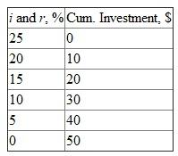
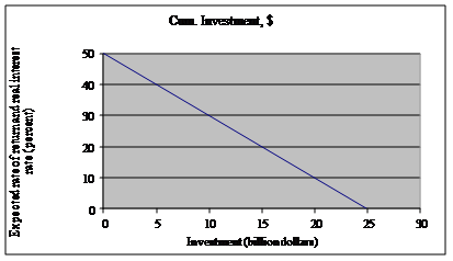 The investment project will be undertaken if its expected rate of return, r , exceeds the real interest rate, it.
a. If i is 15%, business will undertake all investment until the 15% rate of return equals the 15% interest rate. The graph reveals that $20 billion of investment projects have an expected rate of return of 15% or more.
b. If i is 10%, $30 billion of investment projects have an expected rate of return of 10% or more; that is, at a financial price of 10%, $30 billion of investment goods will be demanded.
c. If i is 5%, $40 billion of investment projects have an expected rate of return of 5% or more. The amount of investment for which r equals or exceeds i is $40 billion. Thus, firms will demand $40 billion of investment goods.
The investment project will be undertaken if its expected rate of return, r , exceeds the real interest rate, it.a. If i is 15%, business will undertake all investment until the 15% rate of return equals the 15% interest rate. The graph reveals that $20 billion of investment projects have an expected rate of return of 15% or more.
b. If i is 10%, $30 billion of investment projects have an expected rate of return of 10% or more; that is, at a financial price of 10%, $30 billion of investment goods will be demanded.
c. If i is 5%, $40 billion of investment projects have an expected rate of return of 5% or more. The amount of investment for which r equals or exceeds i is $40 billion. Thus, firms will demand $40 billion of investment goods.
3
What is the multiplier effect What relationship does the MPC bear to the size of the multiplier The MPS What will the multiplier be when the MPS is 0,.4,.6, and 1 What will it be when the MPC is 1,.9,.67,.5, and 0 How much of a change in GDP will result if firms increase their level of investment by $8 billion and the MPC is.80 If the MPC is.67
MPS is the marginal propensity to save. The multiplier is the ratio of change in real GDP to initial change in spending.
 The fractions of an increase in income consumed and saved determine the cumulative spending effects of any initial change in spending and therefore determine the size of the multiplier. The MPC and the multiplier are directly related and the MPS and the multiplier are inversely related. The precise formulas are as shown in the next two equations:
 or
or
 a. When MPS is 0, 0.4, 0.6 and 1, the corresponding multipliers are calculated below:
 When MPS is 0.4
 When MPS is 0.6
 When MPS is 1
 When MPC is 1, 0.9, 0.67, 0.5, multiplier is calculated as follows:
 When MPC is 0.9, multiplier is calculated as follows:
 When MPC is 0.67, multiplier is calculated as follows:
 When MPC is 0.5, multiplier is calculated as follows:
 When MPC is 0, multiplier is calculated as follows:
 Multiplier determines how much GDP will change in accordance with the change in spending, which depends on MPC.

 If the MPC is 0.67, the change in GDP is calculated as follows:


The fractions of an increase in income consumed and saved determine the cumulative spending effects of any initial change in spending and therefore determine the size of the multiplier. The MPC and the multiplier are directly related and the MPS and the multiplier are inversely related. The precise formulas are as shown in the next two equations: or a. When MPS is 0, 0.4, 0.6 and 1, the corresponding multipliers are calculated below: When MPS is 0.4 When MPS is 0.6 When MPS is 1 When MPC is 1, 0.9, 0.67, 0.5, multiplier is calculated as follows: When MPC is 0.9, multiplier is calculated as follows: When MPC is 0.67, multiplier is calculated as follows: When MPC is 0.5, multiplier is calculated as follows: When MPC is 0, multiplier is calculated as follows: Multiplier determines how much GDP will change in accordance with the change in spending, which depends on MPC. If the MPC is 0.67, the change in GDP is calculated as follows: 4
Explain: "Unemployment can be caused by a decrease of aggregate demand or a decrease of aggregate supply." In each case, specify the price-level outcomes.
فتح الحزمة
افتح القفل للوصول البطاقات البالغ عددها 21 في هذه المجموعة.
فتح الحزمة
k this deck
5
The AD curve slopes downward because:
A) per-unit production costs fall as real GDP increases.
B) the income and substitution effects are at work.
C) changes in the determinants of AD alter the amounts of real GDP demanded at each price level.
D) decreases in the price level give rise to real-balances effects, interest-rate effects, and foreign purchases effects that increase the amounts of real GDP demanded.
فتح الحزمة
افتح القفل للوصول البطاقات البالغ عددها 21 في هذه المجموعة.
فتح الحزمة
k this deck
6
Use shifts of the AD and AS curves to explain ( a ) the U.S. experience of strong economic growth, full employment, and price stability in the late 1990s and early 2000s and ( b ) how a strong negative wealth effect from, say, a precipitous drop in the stock market could cause a recession even though productivity is surging.
فتح الحزمة
افتح القفل للوصول البطاقات البالغ عددها 21 في هذه المجموعة.
فتح الحزمة
k this deck
7
Why is the aggregate demand curve downsloping Specify how your explanation differs from the explanation for the downsloping demand curve for a single product. What role does the multiplier play in shifts of the aggregate demand curve
فتح الحزمة
افتح القفل للوصول البطاقات البالغ عددها 21 في هذه المجموعة.
فتح الحزمة
k this deck
8
In early 2001 investment spending sharply declined in the United States. In the 2 months following the September 11, 2001, attacks on the United States, consumption also declined. Use AD-AS analysis to show the two impacts on real GDP.
فتح الحزمة
افتح القفل للوصول البطاقات البالغ عددها 21 في هذه المجموعة.
فتح الحزمة
k this deck
9
FEELING WEALTHIER; SPENDING MORE Access the Bureau of Economic Analysis Web site, www.bea.gov , interactively via the National Income and Product Account Tables. From Table 1.2 find the annual levels of real GDP and real consumption for 1996 and 1999. Did consumption increase more rapidly or less rapidly in percentage terms than real GDP At http://dowjones.com in sequence select Dow Jones Industrial Average, Index Data, and Historical Values to find the level of the DJI on June 1, 1996, and June 1, 1999. What was the percentage change in the DJI over that period How might that change help explain your findings about the growth of consumption versus real GDP between 1996 and 1999
فتح الحزمة
افتح القفل للوصول البطاقات البالغ عددها 21 في هذه المجموعة.
فتح الحزمة
k this deck
10
LAST WORD Go to the OPEC Web site, www.opec.org , and find the current "OPEC basket price" of oil. By clicking on that amount, you will find the annual prices of oil for the past 5 years. By what percentage is the current price higher or lower than 5 years ago Next, go to the Bureau of Economic Analysis Web site, www.bea.gov , and use the interactive feature to find U.S. real GDP for the past years. By what percentage is real GDP higher or lower than it was 5 years ago What if, anything, can you conclude about the relationship between the price of oil and the level of real GDP in the United States
فتح الحزمة
افتح القفل للوصول البطاقات البالغ عددها 21 في هذه المجموعة.
فتح الحزمة
k this deck
11
The AS curve slopes upward because:
A) per-unit production costs rise as real GDP expands toward and beyond its full-employment level.
B) the income and substitution effects are at work.
C) changes in the determinants of AS alter the amounts of real GDP supplied at each price level.
D) increases in the price level give rise to real-balances effects, interest-rate effects, and foreign purchases effects that increase the amounts of real GDP supplied.
فتح الحزمة
افتح القفل للوصول البطاقات البالغ عددها 21 في هذه المجموعة.
فتح الحزمة
k this deck
12
Explain carefully: "A change in the price level shifts the aggregate expenditures curve but not the aggregate demand curve."
فتح الحزمة
افتح القفل للوصول البطاقات البالغ عددها 21 في هذه المجموعة.
فتح الحزمة
k this deck
13
Distinguish between "real-balances effect" and "wealth effect," as the terms are used in this chapter. How does each relate to the aggregate demand curve
فتح الحزمة
افتح القفل للوصول البطاقات البالغ عددها 21 في هذه المجموعة.
فتح الحزمة
k this deck
14
Suppose that the price level is constant and that investment decreases sharply. How would you show this decrease in the aggregate expenditures model What would be the outcome for real GDP How would you show this fall in investment in the aggregate demand-aggregate supply model, assuming the economy is operating in what, in effect, is a horizontal section of the aggregate supply curve
فتح الحزمة
افتح القفل للوصول البطاقات البالغ عددها 21 في هذه المجموعة.
فتح الحزمة
k this deck
15
THE RECESSION OF 2001-WHICH COMPONENT OF AD DECLINED THE MOST Use the interactive feature of the Bureau of Economic Analysis Web site, www.bea.gov , to access the National Income and Product Account Tables. From Table 1.2 find the levels of real GDP, personal consumption expenditures ( C ), gross private investment ( I g ), net exports ( X n ), and government consumption expenditures and gross investment ( G ) in the first and third quarters of 2001. By what percentage did real GDP decline over this period Which of the four broad components of aggregate demand decreased by the largest percentage amount
فتح الحزمة
افتح القفل للوصول البطاقات البالغ عددها 21 في هذه المجموعة.
فتح الحزمة
k this deck
16
At price level 92:
A) a GDP surplus of $12 billion occurs that drives the price level up to 100.
B) a GDP shortage of $12 billion occurs that drives the price level up to 100.
C) the aggregate amount of real GDP demanded is less than the aggregate amount of GDP supplied.
D) the economy is operating beyond its capacity to produce.
فتح الحزمة
افتح القفل للوصول البطاقات البالغ عددها 21 في هذه المجموعة.
فتح الحزمة
k this deck
17
Why is the long-run aggregate supply curve vertical Explain the shape of the short-run aggregate supply curve. Why is the short-run curve relatively flat to the left of the full-employment output and relatively steep to the right
فتح الحزمة
افتح القفل للوصول البطاقات البالغ عددها 21 في هذه المجموعة.
فتح الحزمة
k this deck
18
Suppose real output demanded rises by $4 billion at each price level. The new equilibrium price level will be:
A) 108.
B) 104.
C) 96.
D) 92.
A) 108.
B) 104.
C) 96.
D) 92.
فتح الحزمة
افتح القفل للوصول البطاقات البالغ عددها 21 في هذه المجموعة.
فتح الحزمة
k this deck
19
KEY QUESTION Suppose that the aggregate demand and supply schedules for a hypothetical economy are as shown below:
a. Use these sets of data to graph the aggregate demand and aggregate supply curves. What is the equilibrium price level and the equilibrium level of real output in this hypothetical economy Is the equilibrium real output also necessarily the full-employment real output Explain.
b. Why will a price level of 150 not be an equilibrium price level in this economy Why not 250
c. Suppose that buyers desire to purchase $200 billion of extra real output at each price level. Sketch in the new aggregate demand curve as AD 1. What factors might cause this change in aggregate demand What is the new equilibrium price level and level of real output
فتح الحزمة
افتح القفل للوصول البطاقات البالغ عددها 21 في هذه المجموعة.
فتح الحزمة
k this deck
20
Complete the accompanying table.
Data for completing the table (top to bottom). Consumption: $244; $260; $276; $292; $308; $324; $340; $356; $372. APC: 1.02; 1.00;.99;.97;.96;.95;.94;.94;.93. APS: -.02;.00;.01;.03;.04;.05;.06;.06;.07. MPC:.80 throughout. MPS:.20 throughout.
a. Show the consumption and saving schedules graphically.
b. Find the break even level of income. Explain how is it possible for households to dissave at very low income levels.
c. If the proportion of total income consumed (APC) decreases and the proportion saved (APS) increases as income rises, explain both verbally and graphically how the MPC and MPS can be constant at various levels of income.
فتح الحزمة
افتح القفل للوصول البطاقات البالغ عددها 21 في هذه المجموعة.
فتح الحزمة
k this deck
21
KEY QUESTION What effects would each of the following have on aggregate demand or aggregate supply In each case use a diagram to show the expected effects on the equilibrium price level and the level of real output. Assume all other things remain constant.
a. A widespread fear of depression on the part of consumers.
b. A $2 increase in the excise tax on a pack of cigarettes.
c. A reduction in interest rates at each price level.
d. A major increase in Federal spending for health care.
e. The expectation of rapid inflation.
f. The complete disintegration of OPEC, causing oil prices to fall by one-half.
g. A 10 percent reduction in personal income tax rates.
h. A sizable increase in labor productivity (with no change in nominal wages).
i. A 12 percent increase in nominal wages (with no change in productivity).
j. Depreciation in the international value of the dollar.
فتح الحزمة
افتح القفل للوصول البطاقات البالغ عددها 21 في هذه المجموعة.
فتح الحزمة
k this deck
فتح الحزمة
افتح القفل للوصول البطاقات البالغ عددها 21 في هذه المجموعة.


