Deck 15: Estimation of Dynamic Causal Effects
ملء الشاشة (f)
سؤال
In this exercise you will estimate the effect of oil prices on macroeconomic activity using monthly data on the Index of Industrial Production (IP) and the monthly measure of O, described in Exercise 15.1. The data can be found on the textbook Web site www.pearsonhighered.com/stock_watson in the file USMacroJVlonthly.
a. Compute the monthly growth rate in IP expressed in percentage points, What are the mean and standard deviation of ip_growth over the 1952:1-2009:12 sample period
b. Plot the value of O t Why are so many values of O t equal to zero Why aren't some values of O t negative
c. Estimate a distributed lag model of ip_growth onto current and 18 lagged values of O r What value of the HAC standard truncation parameter m did you choose Why
d. Taken as a group, are the coefficients on O t statistically significantly different from zero
e. Construct graphs like those in Figure 15.2 showing the estimated dynamic multipliers, cumulative multipliers, and 95% confidence intervals. Comment on the real-world size of the multipliers.
f. Suppose that high demand in the United States (evidenced by large values of ip_growth) leads to increases in oil prices. Is O i exogenous Are the estimated multipliers shown in the graphs in (e) reliable Explain.
Exercise
Increases in oil prices have been blamed for several recessions in developed countries. To quantify the effect of oil prices on real economic activity, researchers have done regressions like those discussed in this chapter. Let GDP t denote the value of quarterly gross domestic product in the United States and let Y t =(Q\n(GDP t / GDP t-1 ) be the quarterly percentage change in GDP. James Hamilton, an econometrician and macroeconomist, has suggested that oil prices adversely affect that economy only when they jump above their values in the recent past. Specifically, let O, equal the greater of zero or the percentage point difference between oil prices at date t and their maximum value during the past year. A distributed lag regression relating Y t and O t estimated over 1955:1-2000:IV, is

a. Suppose that oil prices jump 25% above their previous peak value and stay at this new higher level (so that O t = 25 and O t+1 = O t+2 = • • • = 0). What is the predicted effect on output growth for each quarter over the next 2 years
b. Construct a 95% confidence interval for your answers in (a).
c. What is the predicted cumulative change in GDP growth over eight quarters
d. The HAC F-statistic testing whether the coefficients on O t and its lags are zero is 3.49. Are the coefficients significantly different from zero
a. Compute the monthly growth rate in IP expressed in percentage points, What are the mean and standard deviation of ip_growth over the 1952:1-2009:12 sample period
b. Plot the value of O t Why are so many values of O t equal to zero Why aren't some values of O t negative
c. Estimate a distributed lag model of ip_growth onto current and 18 lagged values of O r What value of the HAC standard truncation parameter m did you choose Why
d. Taken as a group, are the coefficients on O t statistically significantly different from zero
e. Construct graphs like those in Figure 15.2 showing the estimated dynamic multipliers, cumulative multipliers, and 95% confidence intervals. Comment on the real-world size of the multipliers.
f. Suppose that high demand in the United States (evidenced by large values of ip_growth) leads to increases in oil prices. Is O i exogenous Are the estimated multipliers shown in the graphs in (e) reliable Explain.
Exercise
Increases in oil prices have been blamed for several recessions in developed countries. To quantify the effect of oil prices on real economic activity, researchers have done regressions like those discussed in this chapter. Let GDP t denote the value of quarterly gross domestic product in the United States and let Y t =(Q\n(GDP t / GDP t-1 ) be the quarterly percentage change in GDP. James Hamilton, an econometrician and macroeconomist, has suggested that oil prices adversely affect that economy only when they jump above their values in the recent past. Specifically, let O, equal the greater of zero or the percentage point difference between oil prices at date t and their maximum value during the past year. A distributed lag regression relating Y t and O t estimated over 1955:1-2000:IV, is
a. Suppose that oil prices jump 25% above their previous peak value and stay at this new higher level (so that O t = 25 and O t+1 = O t+2 = • • • = 0). What is the predicted effect on output growth for each quarter over the next 2 years
b. Construct a 95% confidence interval for your answers in (a).
c. What is the predicted cumulative change in GDP growth over eight quarters
d. The HAC F-statistic testing whether the coefficients on O t and its lags are zero is 3.49. Are the coefficients significantly different from zero
سؤال
سؤال
Macroeconomists have also noticed that interest rates change following oil price jumps. Let R t denote the interest rate on 3-month Treasury bills (in percentage points at an annual rate). The distributed lag regression relating the change in R t ( R t ) to O t estimated over 1955:1-2000:IV is
a. Suppose that oil prices jump 25% above their previous peak value and stay at this new higher level (so that O t = 25 and O t+l = O t +2 = • • • = 0). What is the predicted change in interest rates for each quarter over the next 2 years
b. Construct 95% confidence intervals for your answers to (a).
c. What is the effect of this change in oil prices on the level of interest rates in period t + 8 How is your answer related to the cumulative multiplier
d. The HAC F-statistic testing whether the coefficients on O t and its lags are zero is 4.25. Are the coefficients significantly different from zero
سؤال
In the data file USMacro_Monthly, you will find data on two aggregate price series for the United States: the Consumer Price Index (CPI) and the Personal Consumption Expenditures Deflator (PCED). These series are alternative measures of consumer prices in the United States. The CPI prices a basket of goods whose composition is updated every 5-10 years. The PCED uses chain-weighting to price a basket of goods whose composition changes from month to month. Economists have argued that the CPI will overstate inflation because it does not take into account the substitution that occurs when relative prices change. If this substitution bias is important, then average CPI inflation should be systematically higher than PCED inflation. Let
 , is the monthly rate of price inflation (measured in percentage points at an annual rate) based on the CPI, is the monthly rate of price inflation from the PCED, and Y i is the difference. Using data from 1970:1 through 2009:12, carry out the following exercises.
a. Compute the sample means of Are these point estimates consistent with the presence of economically significant substitution bias in the CPI
b. Compute the sample mean of Y t. Explain why it is numerically equal to the difference in the means computed in (a).
c. Show that the population mean of Y is equal to the difference of the population means of the two inflation rates.
d. Consider the "constant-term-only" regression:
 . Show that
 . Do you think that u, is serially correlated Explain.
e. Construct a 95% confidence interval for 0. What value of the HAC standard truncation parameter m did you choose Why
f. Is there statistically significant evidence that the mean inflation rate for the CPI is greater than the rate for the PCED
g. Is there evidence of instability in 0 Carry out a QLR test.
, is the monthly rate of price inflation (measured in percentage points at an annual rate) based on the CPI, is the monthly rate of price inflation from the PCED, and Y i is the difference. Using data from 1970:1 through 2009:12, carry out the following exercises.a. Compute the sample means of Are these point estimates consistent with the presence of economically significant substitution bias in the CPI
b. Compute the sample mean of Y t. Explain why it is numerically equal to the difference in the means computed in (a).
c. Show that the population mean of Y is equal to the difference of the population means of the two inflation rates.
d. Consider the "constant-term-only" regression:
. Show that . Do you think that u, is serially correlated Explain. e. Construct a 95% confidence interval for 0. What value of the HAC standard truncation parameter m did you choose Why
f. Is there statistically significant evidence that the mean inflation rate for the CPI is greater than the rate for the PCED
g. Is there evidence of instability in 0 Carry out a QLR test.
سؤال
سؤال
Consider two different randomized experiments. In experiment A, oil prices are set randomly and the central bank reacts according to its usual policy rules in response to economic conditions, including changes in the oil price. In experiment B, oil prices are set randomly and the central bank holds interest rates constant and in particular does not respond to the oil price changes. In both, GDP growth is observed. Now suppose that oil prices are exogenous in the regression in Exercise 15.1.To which experiment, A or B, does the dynamic causal effect estimated in Exercise 15.1 correspond
Exercise
Increases in oil prices have been blamed for several recessions in developed countries. To quantify the effect of oil prices on real economic activity, researchers have done regressions like those discussed in this chapter. Let GDP t denote the value of quarterly gross domestic product in the United States and let Y t =(Q\n(GDP t / GDP t-1 ) be the quarterly percentage change in GDP. James Hamilton, an econometrician and macroeconomist, has suggested that oil prices adversely affect that economy only when they jump above their values in the recent past. Specifically, let O, equal the greater of zero or the percentage point difference between oil prices at date t and their maximum value during the past year. A distributed lag regression relating Y t and O t estimated over 1955:1-2000:IV, is
a. Suppose that oil prices jump 25% above their previous peak value and stay at this new higher level (so that O t = 25 and O t+l = O t +2 = • • • = 0). What is the predicted change in interest rates for each quarter over the next 2 years
b. Construct 95% confidence intervals for your answers to (a).
c. What is the effect of this change in oil prices on the level of interest rates in period t + 8 How is your answer related to the cumulative multiplier
d. The HAC F-statistic testing whether the coefficients on O t and its lags are zero is 4.25. Are the coefficients significantly different from zero
سؤال
سؤال
Suppose that oil prices are strictly exogenous. Discuss how you could improve on the estimates of the dynamic multipliers in Exercise 15.1.
Exercise
Increases in oil prices have been blamed for several recessions in developed countries. To quantify the effect of oil prices on real economic activity, researchers have done regressions like those discussed in this chapter. Let GDP t denote the value of quarterly gross domestic product in the United States and let Y t =(Q\n(GDP t / GDP t-1 ) be the quarterly percentage change in GDP. James Hamilton, an econometrician and macroeconomist, has suggested that oil prices adversely affect that economy only when they jump above their values in the recent past. Specifically, let O, equal the greater of zero or the percentage point difference between oil prices at date t and their maximum value during the past year. A distributed lag regression relating Y t and O t estimated over 1955:1-2000:IV, is

a. Suppose that oil prices jump 25% above their previous peak value and stay at this new higher level (so that O t = 25 and O t+1 = O t+2 = • • • = 0). What is the predicted effect on output growth for each quarter over the next 2 years
b. Construct a 95% confidence interval for your answers in (a)..
c. What is the predicted cumulative change in GDP growth over eight quarters .
d. The HAC F-statistic testing whether the coefficients on O t and its lags are zero is 3.49. Are the coefficients significantly different from zero
Exercise
Increases in oil prices have been blamed for several recessions in developed countries. To quantify the effect of oil prices on real economic activity, researchers have done regressions like those discussed in this chapter. Let GDP t denote the value of quarterly gross domestic product in the United States and let Y t =(Q\n(GDP t / GDP t-1 ) be the quarterly percentage change in GDP. James Hamilton, an econometrician and macroeconomist, has suggested that oil prices adversely affect that economy only when they jump above their values in the recent past. Specifically, let O, equal the greater of zero or the percentage point difference between oil prices at date t and their maximum value during the past year. A distributed lag regression relating Y t and O t estimated over 1955:1-2000:IV, is
a. Suppose that oil prices jump 25% above their previous peak value and stay at this new higher level (so that O t = 25 and O t+1 = O t+2 = • • • = 0). What is the predicted effect on output growth for each quarter over the next 2 years
b. Construct a 95% confidence interval for your answers in (a)..
c. What is the predicted cumulative change in GDP growth over eight quarters .
d. The HAC F-statistic testing whether the coefficients on O t and its lags are zero is 3.49. Are the coefficients significantly different from zero
سؤال
سؤال
سؤال
Consider the regression model Y t = 0 + 1 X t + u t where u, follows the stationary AR(1) mode with
 . with mean 0 and variance and |
1 | 1, the regressor X t follows the stationary AR(1) mode with e t i.i.d. with mean 0 and variance and | 1 | 1, and e t is independent of for all t and i.
a. Show that var and var( X t ) =
 .
.
b. Show that cov and cov
 .
.
c. Show that corr and corr
 .
.
d. Consider the terms and f T in Equation (15.14).
i. Show that where is the variance of X and
 , is the variance of u.
ii. Derive an expression for f
. with mean 0 and variance and |1 | 1, the regressor X t follows the stationary AR(1) mode with e t i.i.d. with mean 0 and variance and | 1 | 1, and e t is independent of for all t and i.
a. Show that var and var( X t ) =
.b. Show that cov and cov
.c. Show that corr and corr
.d. Consider the terms and f T in Equation (15.14).
i. Show that where is the variance of X and
, is the variance of u. ii. Derive an expression for f
سؤال
Consider the regression model where u t follows the stationary AR(1) model
 , with
 , i.i.d. with mean 0 and variance
a. Suppose that X t is independent of for all t and j. Is X t exogenous (past and present) Is X t strictly exogenous (past, present, and future) .
b. Suppose that Is X t exogenous Is X t strictly exogenous
, with , i.i.d. with mean 0 and variance a. Suppose that X t is independent of for all t and j. Is X t exogenous (past and present) Is X t strictly exogenous (past, present, and future) .
b. Suppose that Is X t exogenous Is X t strictly exogenous
سؤال
Consider the model in Exercise 15.7 with

a. Is the OLS estimator of 1 consistent Explain..
b. Explain why the GLS estimator of 1 is not consistent..
c. Show that the infeasible GLS estimator
a. Is the OLS estimator of 1 consistent Explain..
b. Explain why the GLS estimator of 1 is not consistent..
c. Show that the infeasible GLS estimator
سؤال
Consider the "constant-term-only" regression model Y 1 = 0 + u 1 where u follows the stationary AR(1) model
 0 and variance
 .
.
0 and variance . سؤال
سؤال
Increases in oil prices have been blamed for several recessions in developed countries. To quantify the effect of oil prices on real economic activity, researchers have done regressions like those discussed in this chapter. Let GDP t denote the value of quarterly gross domestic product in the United States and let Y t =(Q\n(GDP t / GDP t-1 ) be the quarterly percentage change in GDP. James Hamilton, an econometrician and macroeconomist, has suggested that oil prices adversely affect that economy only when they jump above their values in the recent past. Specifically, let O, equal the greater of zero or the percentage point difference between oil prices at date t and their maximum value during the past year. A distributed lag regression relating Y t and O t estimated over 1955:1-2000:IV, is

a. Suppose that oil prices jump 25% above their previous peak value and stay at this new higher level (so that O t = 25 and O t+1 = O t+2 = • • • = 0). What is the predicted effect on output growth for each quarter over the next 2 years
b. Construct a 95% confidence interval for your answers in (a).
c. What is the predicted cumulative change in GDP growth over eight quarters
d. The HAC F-statistic testing whether the coefficients on O t and its lags are zero is 3.49. Are the coefficients significantly different from zero

فتح الحزمة
قم بالتسجيل لفتح البطاقات في هذه المجموعة!
Unlock Deck
Unlock Deck
1/16
العب
ملء الشاشة (f)
Deck 15: Estimation of Dynamic Causal Effects
1
In this exercise you will estimate the effect of oil prices on macroeconomic activity using monthly data on the Index of Industrial Production (IP) and the monthly measure of O, described in Exercise 15.1. The data can be found on the textbook Web site www.pearsonhighered.com/stock_watson in the file USMacroJVlonthly.
a. Compute the monthly growth rate in IP expressed in percentage points, What are the mean and standard deviation of ip_growth over the 1952:1-2009:12 sample period
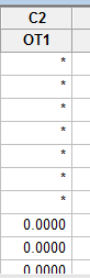
b. Plot the value of O t Why are so many values of O t equal to zero Why aren't some values of O t negative
c. Estimate a distributed lag model of ip_growth onto current and 18 lagged values of O r What value of the HAC standard truncation parameter m did you choose Why
d. Taken as a group, are the coefficients on O t statistically significantly different from zero
e. Construct graphs like those in Figure 15.2 showing the estimated dynamic multipliers, cumulative multipliers, and 95% confidence intervals. Comment on the real-world size of the multipliers.
f. Suppose that high demand in the United States (evidenced by large values of ip_growth) leads to increases in oil prices. Is O i exogenous Are the estimated multipliers shown in the graphs in (e) reliable Explain.
Exercise
Increases in oil prices have been blamed for several recessions in developed countries. To quantify the effect of oil prices on real economic activity, researchers have done regressions like those discussed in this chapter. Let GDP t denote the value of quarterly gross domestic product in the United States and let Y t =(Q\n(GDP t / GDP t-1 ) be the quarterly percentage change in GDP. James Hamilton, an econometrician and macroeconomist, has suggested that oil prices adversely affect that economy only when they jump above their values in the recent past. Specifically, let O, equal the greater of zero or the percentage point difference between oil prices at date t and their maximum value during the past year. A distributed lag regression relating Y t and O t estimated over 1955:1-2000:IV, is
a. Suppose that oil prices jump 25% above their previous peak value and stay at this new higher level (so that O t = 25 and O t+1 = O t+2 = • • • = 0). What is the predicted effect on output growth for each quarter over the next 2 years
b. Construct a 95% confidence interval for your answers in (a).
c. What is the predicted cumulative change in GDP growth over eight quarters
d. The HAC F-statistic testing whether the coefficients on O t and its lags are zero is 3.49. Are the coefficients significantly different from zero
a. Compute the monthly growth rate in IP expressed in percentage points, What are the mean and standard deviation of ip_growth over the 1952:1-2009:12 sample period
b. Plot the value of O t Why are so many values of O t equal to zero Why aren't some values of O t negative
c. Estimate a distributed lag model of ip_growth onto current and 18 lagged values of O r What value of the HAC standard truncation parameter m did you choose Why
d. Taken as a group, are the coefficients on O t statistically significantly different from zero
e. Construct graphs like those in Figure 15.2 showing the estimated dynamic multipliers, cumulative multipliers, and 95% confidence intervals. Comment on the real-world size of the multipliers.
f. Suppose that high demand in the United States (evidenced by large values of ip_growth) leads to increases in oil prices. Is O i exogenous Are the estimated multipliers shown in the graphs in (e) reliable Explain.
Exercise
Increases in oil prices have been blamed for several recessions in developed countries. To quantify the effect of oil prices on real economic activity, researchers have done regressions like those discussed in this chapter. Let GDP t denote the value of quarterly gross domestic product in the United States and let Y t =(Q\n(GDP t / GDP t-1 ) be the quarterly percentage change in GDP. James Hamilton, an econometrician and macroeconomist, has suggested that oil prices adversely affect that economy only when they jump above their values in the recent past. Specifically, let O, equal the greater of zero or the percentage point difference between oil prices at date t and their maximum value during the past year. A distributed lag regression relating Y t and O t estimated over 1955:1-2000:IV, is
a. Suppose that oil prices jump 25% above their previous peak value and stay at this new higher level (so that O t = 25 and O t+1 = O t+2 = • • • = 0). What is the predicted effect on output growth for each quarter over the next 2 years
b. Construct a 95% confidence interval for your answers in (a).
c. What is the predicted cumulative change in GDP growth over eight quarters
d. The HAC F-statistic testing whether the coefficients on O t and its lags are zero is 3.49. Are the coefficients significantly different from zero
Consider the table:
 a.
a.
In order to compute the value of monthly growth rate we use the formula:
 We get:
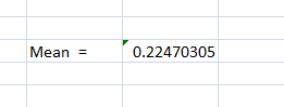
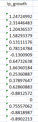 For mean:
1. Click on Formulas tab on toolbar and go to AutoSum group. Now click on more functions.
2. Now find and click on Average. Click OK.
 3. In the dialogue box, enter the numbers whose average is needed. Click on empty box near Number1 to enter the number. In order to enter the value, drag along the data to select cells.
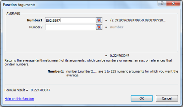 4. Click on OK.
The output of which will be:
 For Standard deviation:
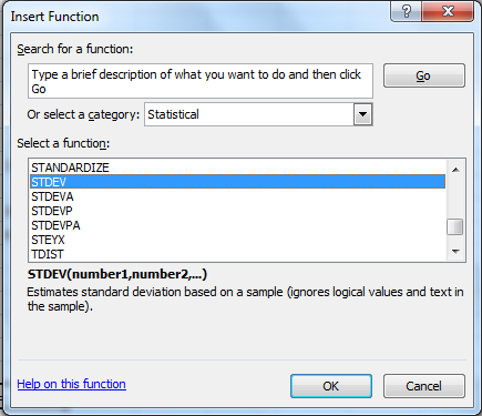
1. Click on Formulas tab on toolbar and go to More Functions and then Statistics group. Now click on Insert functions.
2. Now find and click on STDEV. Click OK.
 3. In the dialogue box, enter the numbers whose standard deviation is needed. Click on empty box near Number1 to enter the number. In order to enter the value, drag along the data to select cells.
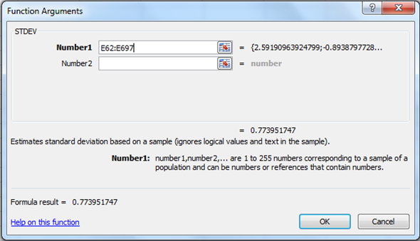 4. Click on OK. It gives the output:
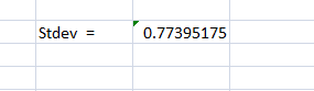 The units of growth rate in IP are percentage per month.
b.
In order to plot the values of
 , follow the steps:
1. Copy the columns from excel to Minitab worksheet
 3. Go to Graph , and then Scatter plot. Then go to with connect line. Click OK.
 4. Now click on variable which will correspond to y and using select , import it there. Similarly, import for x.
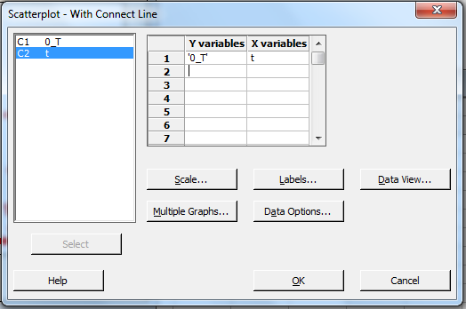 5. Click OK. Output is:
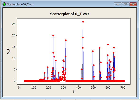
 Is the greater of zero or the percentage point difference between oil prices at date t and their maximum value during the past year. Thus
 , and
, and
 if the date t is not greater than the maximum value over the past year
c.
To compute the distributed lag model, we first need to calculate the lagged values:
1. Go to Stat , and then Time Series.
3. Click on lag.
4. Enter the series to find the lag and enter the name of the variable. Enter the lag value 1.
Click OK.
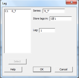 5. Output is:
 Similarly, we compute the rest 17 lags.
Now, run regression:
1. Go to Stat , and then Regression. Then go to Regression again.
2. Now click on variable which will correspond to y and using select , import it there. Similarly, import for x.
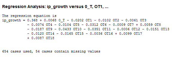
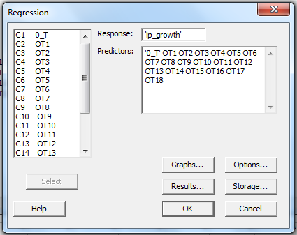 8. Cick OK. Output is:
 The value of the HAC standard truncation parameter m is:
 Where T is the sample size i.e. 708.
Now,
 Hence, the value of m is 7.
d.
Now, F- test is applied to test the slope coefficients of regression equation in equation (2), for which the null hypothesis (hypothesis of no difference) is,
 Where,
 and the alternative hypothesis, against the null hypothesis, is,
 Now, using the "regression output", it is observed that the P-value corresponding to value of F statistic is 0.000 as shown below,
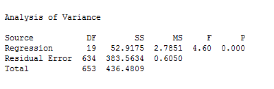 So, P-value (0.00) is less than the level of significance, say 0.05, so the null hypothesis is rejected and it is concluded that the all the slope coefficients
 are significantly different from zero.
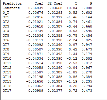 However, in the regression output, the P-value corresponding to the intercept term (constant) is 0.00 which is lesser than level of significance, say 0.05, so the constant is significantly different from zero.
e.
Graph:
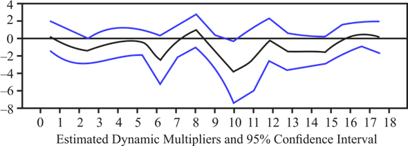
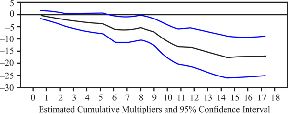 The cumulative multipliers show a persistent and large decrease in industrial production following an increase in oil prices above their previous 12 month peak price. Specifically a 100% increase in oil prices is leads to an estimated 17% decline in industrial production after
18 months
f.
No.
 is not exogenous. Results in part (e) are not reliable.
a.In order to compute the value of monthly growth rate we use the formula:
We get: For mean:1. Click on Formulas tab on toolbar and go to AutoSum group. Now click on more functions.
2. Now find and click on Average. Click OK.
3. In the dialogue box, enter the numbers whose average is needed. Click on empty box near Number1 to enter the number. In order to enter the value, drag along the data to select cells. 4. Click on OK.The output of which will be:
For Standard deviation:1. Click on Formulas tab on toolbar and go to More Functions and then Statistics group. Now click on Insert functions.
2. Now find and click on STDEV. Click OK.
3. In the dialogue box, enter the numbers whose standard deviation is needed. Click on empty box near Number1 to enter the number. In order to enter the value, drag along the data to select cells. 4. Click on OK. It gives the output: The units of growth rate in IP are percentage per month.b.
In order to plot the values of
, follow the steps:1. Copy the columns from excel to Minitab worksheet
3. Go to Graph , and then Scatter plot. Then go to with connect line. Click OK. 4. Now click on variable which will correspond to y and using select , import it there. Similarly, import for x. 5. Click OK. Output is: Is the greater of zero or the percentage point difference between oil prices at date t and their maximum value during the past year. Thus , and if the date t is not greater than the maximum value over the past yearc.
To compute the distributed lag model, we first need to calculate the lagged values:
1. Go to Stat , and then Time Series.
3. Click on lag.
4. Enter the series to find the lag and enter the name of the variable. Enter the lag value 1.
Click OK.
5. Output is: Similarly, we compute the rest 17 lags.Now, run regression:
1. Go to Stat , and then Regression. Then go to Regression again.
2. Now click on variable which will correspond to y and using select , import it there. Similarly, import for x.
8. Cick OK. Output is: The value of the HAC standard truncation parameter m is: Where T is the sample size i.e. 708.Now,
Hence, the value of m is 7.d.
Now, F- test is applied to test the slope coefficients of regression equation in equation (2), for which the null hypothesis (hypothesis of no difference) is,
Where, and the alternative hypothesis, against the null hypothesis, is, Now, using the "regression output", it is observed that the P-value corresponding to value of F statistic is 0.000 as shown below, So, P-value (0.00) is less than the level of significance, say 0.05, so the null hypothesis is rejected and it is concluded that the all the slope coefficients are significantly different from zero. However, in the regression output, the P-value corresponding to the intercept term (constant) is 0.00 which is lesser than level of significance, say 0.05, so the constant is significantly different from zero.e.
Graph:
The cumulative multipliers show a persistent and large decrease in industrial production following an increase in oil prices above their previous 12 month peak price. Specifically a 100% increase in oil prices is leads to an estimated 17% decline in industrial production after18 months
f.
No.
is not exogenous. Results in part (e) are not reliable. 2
In the 1970s a common practice was to estimate a distributed lag model relating changes in nominal gross domestic product ( Y ) to current and past changes in the money supply ( X ). Under what assumptions will this regression estimate the causal effects of money on nominal GDP Are these assumptions likely to be satisfied in a modern economy like that of the United States
The ADL distributed lag model is valid when the independent variables are exogenous. In the case of regression for economic growth to changes money supply X , money supply is not exogenous. Most modern economies have a central bank which regulates the inflation rate; hence they can change money supply. The central banks act accordingly to economic conditions, for instance if a recession occurs, negative change in GDP, then the central bank may increase money supply to improve short term economic conditions.
3
Macroeconomists have also noticed that interest rates change following oil price jumps. Let R t denote the interest rate on 3-month Treasury bills (in percentage points at an annual rate). The distributed lag regression relating the change in R t ( R t ) to O t estimated over 1955:1-2000:IV is
a. Suppose that oil prices jump 25% above their previous peak value and stay at this new higher level (so that O t = 25 and O t+l = O t +2 = • • • = 0). What is the predicted change in interest rates for each quarter over the next 2 years
b. Construct 95% confidence intervals for your answers to (a).
c. What is the effect of this change in oil prices on the level of interest rates in period t + 8 How is your answer related to the cumulative multiplier
d. The HAC F-statistic testing whether the coefficients on O t and its lags are zero is 4.25. Are the coefficients significantly different from zero
a. Suppose that oil prices jump 25% above their previous peak value and stay at this new higher level (so that O t = 25 and O t+l = O t +2 = • • • = 0). What is the predicted change in interest rates for each quarter over the next 2 years
b. Construct 95% confidence intervals for your answers to (a).
c. What is the effect of this change in oil prices on the level of interest rates in period t + 8 How is your answer related to the cumulative multiplier
d. The HAC F-statistic testing whether the coefficients on O t and its lags are zero is 4.25. Are the coefficients significantly different from zero
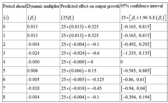
a.
Make a table to predict the change in interest rates for each quarter over the next two years by considering
 as a dynamic multiplier. Therefore, with 25% oil price jump; the growth for ith quarter will be
 percentage points. The table is shown below:
 b.
b.
The 95% confidence interval will compute the change in interest rates for each quarter over the next two years by using formula
 percentage points. The confidence interval is already computed in part a.
c.
The effect of change in oil prices on the level of interest rates in period
 can be computed as shown below:
 d.
d.
Here, consider 1% level of significance so that it can conclude that at 1% critical value for the F -test is 2.407. It is given that HAC F-statistics is 1.93 that is smaller as compare to critical value 2.407. Therefore, it can infer that do not reject the null hypothesis that all the coefficients on
 and its lag are zero at the 1% level.
Make a table to predict the change in interest rates for each quarter over the next two years by considering
as a dynamic multiplier. Therefore, with 25% oil price jump; the growth for ith quarter will be percentage points. The table is shown below: b. The 95% confidence interval will compute the change in interest rates for each quarter over the next two years by using formula
percentage points. The confidence interval is already computed in part a. c.
The effect of change in oil prices on the level of interest rates in period
can be computed as shown below: d. Here, consider 1% level of significance so that it can conclude that at 1% critical value for the F -test is 2.407. It is given that HAC F-statistics is 1.93 that is smaller as compare to critical value 2.407. Therefore, it can infer that do not reject the null hypothesis that all the coefficients on
and its lag are zero at the 1% level. 4
In the data file USMacro_Monthly, you will find data on two aggregate price series for the United States: the Consumer Price Index (CPI) and the Personal Consumption Expenditures Deflator (PCED). These series are alternative measures of consumer prices in the United States. The CPI prices a basket of goods whose composition is updated every 5-10 years. The PCED uses chain-weighting to price a basket of goods whose composition changes from month to month. Economists have argued that the CPI will overstate inflation because it does not take into account the substitution that occurs when relative prices change. If this substitution bias is important, then average CPI inflation should be systematically higher than PCED inflation. Let
, is the monthly rate of price inflation (measured in percentage points at an annual rate) based on the CPI, is the monthly rate of price inflation from the PCED, and Y i is the difference. Using data from 1970:1 through 2009:12, carry out the following exercises.
a. Compute the sample means of Are these point estimates consistent with the presence of economically significant substitution bias in the CPI
b. Compute the sample mean of Y t. Explain why it is numerically equal to the difference in the means computed in (a).
c. Show that the population mean of Y is equal to the difference of the population means of the two inflation rates.
d. Consider the "constant-term-only" regression:
. Show that
. Do you think that u, is serially correlated Explain.
e. Construct a 95% confidence interval for 0. What value of the HAC standard truncation parameter m did you choose Why
f. Is there statistically significant evidence that the mean inflation rate for the CPI is greater than the rate for the PCED
g. Is there evidence of instability in 0 Carry out a QLR test.
, is the monthly rate of price inflation (measured in percentage points at an annual rate) based on the CPI, is the monthly rate of price inflation from the PCED, and Y i is the difference. Using data from 1970:1 through 2009:12, carry out the following exercises.a. Compute the sample means of Are these point estimates consistent with the presence of economically significant substitution bias in the CPI
b. Compute the sample mean of Y t. Explain why it is numerically equal to the difference in the means computed in (a).
c. Show that the population mean of Y is equal to the difference of the population means of the two inflation rates.
d. Consider the "constant-term-only" regression:
. Show that . Do you think that u, is serially correlated Explain. e. Construct a 95% confidence interval for 0. What value of the HAC standard truncation parameter m did you choose Why
f. Is there statistically significant evidence that the mean inflation rate for the CPI is greater than the rate for the PCED
g. Is there evidence of instability in 0 Carry out a QLR test.
فتح الحزمة
افتح القفل للوصول البطاقات البالغ عددها 16 في هذه المجموعة.
فتح الحزمة
k this deck
5
Suppose that X is strictly exogenous. A researcher estimates an ADL(1,1) model, calculates the regression residual, and finds the residual to be highly serially correlated. Should the researcher estimate a new ADL model with additional lags or simply use HAC standard errors for the ADL(1,1) estimated coefficients
فتح الحزمة
افتح القفل للوصول البطاقات البالغ عددها 16 في هذه المجموعة.
فتح الحزمة
k this deck
6
Consider two different randomized experiments. In experiment A, oil prices are set randomly and the central bank reacts according to its usual policy rules in response to economic conditions, including changes in the oil price. In experiment B, oil prices are set randomly and the central bank holds interest rates constant and in particular does not respond to the oil price changes. In both, GDP growth is observed. Now suppose that oil prices are exogenous in the regression in Exercise 15.1.To which experiment, A or B, does the dynamic causal effect estimated in Exercise 15.1 correspond
Exercise
Increases in oil prices have been blamed for several recessions in developed countries. To quantify the effect of oil prices on real economic activity, researchers have done regressions like those discussed in this chapter. Let GDP t denote the value of quarterly gross domestic product in the United States and let Y t =(Q\n(GDP t / GDP t-1 ) be the quarterly percentage change in GDP. James Hamilton, an econometrician and macroeconomist, has suggested that oil prices adversely affect that economy only when they jump above their values in the recent past. Specifically, let O, equal the greater of zero or the percentage point difference between oil prices at date t and their maximum value during the past year. A distributed lag regression relating Y t and O t estimated over 1955:1-2000:IV, is
a. Suppose that oil prices jump 25% above their previous peak value and stay at this new higher level (so that O t = 25 and O t+l = O t +2 = • • • = 0). What is the predicted change in interest rates for each quarter over the next 2 years
b. Construct 95% confidence intervals for your answers to (a).
c. What is the effect of this change in oil prices on the level of interest rates in period t + 8 How is your answer related to the cumulative multiplier
d. The HAC F-statistic testing whether the coefficients on O t and its lags are zero is 4.25. Are the coefficients significantly different from zero
Exercise
Increases in oil prices have been blamed for several recessions in developed countries. To quantify the effect of oil prices on real economic activity, researchers have done regressions like those discussed in this chapter. Let GDP t denote the value of quarterly gross domestic product in the United States and let Y t =(Q\n(GDP t / GDP t-1 ) be the quarterly percentage change in GDP. James Hamilton, an econometrician and macroeconomist, has suggested that oil prices adversely affect that economy only when they jump above their values in the recent past. Specifically, let O, equal the greater of zero or the percentage point difference between oil prices at date t and their maximum value during the past year. A distributed lag regression relating Y t and O t estimated over 1955:1-2000:IV, is
a. Suppose that oil prices jump 25% above their previous peak value and stay at this new higher level (so that O t = 25 and O t+l = O t +2 = • • • = 0). What is the predicted change in interest rates for each quarter over the next 2 years
b. Construct 95% confidence intervals for your answers to (a).
c. What is the effect of this change in oil prices on the level of interest rates in period t + 8 How is your answer related to the cumulative multiplier
d. The HAC F-statistic testing whether the coefficients on O t and its lags are zero is 4.25. Are the coefficients significantly different from zero
فتح الحزمة
افتح القفل للوصول البطاقات البالغ عددها 16 في هذه المجموعة.
فتح الحزمة
k this deck
7
Suppose that a distributed lag regression is estimated, where the dependent variable is Y t instead of Y t. Explain how you would compute the dynamic multipliers of X t on Y t..
فتح الحزمة
افتح القفل للوصول البطاقات البالغ عددها 16 في هذه المجموعة.
فتح الحزمة
k this deck
8
Suppose that oil prices are strictly exogenous. Discuss how you could improve on the estimates of the dynamic multipliers in Exercise 15.1.
Exercise
Increases in oil prices have been blamed for several recessions in developed countries. To quantify the effect of oil prices on real economic activity, researchers have done regressions like those discussed in this chapter. Let GDP t denote the value of quarterly gross domestic product in the United States and let Y t =(Q\n(GDP t / GDP t-1 ) be the quarterly percentage change in GDP. James Hamilton, an econometrician and macroeconomist, has suggested that oil prices adversely affect that economy only when they jump above their values in the recent past. Specifically, let O, equal the greater of zero or the percentage point difference between oil prices at date t and their maximum value during the past year. A distributed lag regression relating Y t and O t estimated over 1955:1-2000:IV, is
a. Suppose that oil prices jump 25% above their previous peak value and stay at this new higher level (so that O t = 25 and O t+1 = O t+2 = • • • = 0). What is the predicted effect on output growth for each quarter over the next 2 years
b. Construct a 95% confidence interval for your answers in (a)..
c. What is the predicted cumulative change in GDP growth over eight quarters .
d. The HAC F-statistic testing whether the coefficients on O t and its lags are zero is 3.49. Are the coefficients significantly different from zero
فتح الحزمة
افتح القفل للوصول البطاقات البالغ عددها 16 في هذه المجموعة.
فتح الحزمة
k this deck
9
Suppose that you added FDD t+1 as an additional regressor in Equation (15.2). If FDD is strictly exogenous, would you expect the coefficient on FDD t+1 to be zero or nonzero Would your answer change if FDD is exogenous but ilot strictly exogenous
فتح الحزمة
افتح القفل للوصول البطاقات البالغ عددها 16 في هذه المجموعة.
فتح الحزمة
k this deck
10
Derive Equation (15.7) from Equation (15.4) and show that 0 = 0 , 1 = 1 , 2 = 1 + , 3 = 1 + 1 + 3 (etc.).
فتح الحزمة
افتح القفل للوصول البطاقات البالغ عددها 16 في هذه المجموعة.
فتح الحزمة
k this deck
11
Consider the regression model Y t = 0 + 1 X t + u t where u, follows the stationary AR(1) mode with
. with mean 0 and variance and |
1 | 1, the regressor X t follows the stationary AR(1) mode with e t i.i.d. with mean 0 and variance and | 1 | 1, and e t is independent of for all t and i.
a. Show that var and var( X t ) =
.
b. Show that cov and cov
.
c. Show that corr and corr
.
d. Consider the terms and f T in Equation (15.14).
i. Show that where is the variance of X and
, is the variance of u.
ii. Derive an expression for f
. with mean 0 and variance and |1 | 1, the regressor X t follows the stationary AR(1) mode with e t i.i.d. with mean 0 and variance and | 1 | 1, and e t is independent of for all t and i.
a. Show that var and var( X t ) =
.b. Show that cov and cov
.c. Show that corr and corr
.d. Consider the terms and f T in Equation (15.14).
i. Show that where is the variance of X and
, is the variance of u. ii. Derive an expression for f
فتح الحزمة
افتح القفل للوصول البطاقات البالغ عددها 16 في هذه المجموعة.
فتح الحزمة
k this deck
12
Consider the regression model where u t follows the stationary AR(1) model
, with
, i.i.d. with mean 0 and variance
a. Suppose that X t is independent of for all t and j. Is X t exogenous (past and present) Is X t strictly exogenous (past, present, and future) .
b. Suppose that Is X t exogenous Is X t strictly exogenous
, with , i.i.d. with mean 0 and variance a. Suppose that X t is independent of for all t and j. Is X t exogenous (past and present) Is X t strictly exogenous (past, present, and future) .
b. Suppose that Is X t exogenous Is X t strictly exogenous
فتح الحزمة
افتح القفل للوصول البطاقات البالغ عددها 16 في هذه المجموعة.
فتح الحزمة
k this deck
13
Consider the model in Exercise 15.7 with
a. Is the OLS estimator of 1 consistent Explain..
b. Explain why the GLS estimator of 1 is not consistent..
c. Show that the infeasible GLS estimator
a. Is the OLS estimator of 1 consistent Explain..
b. Explain why the GLS estimator of 1 is not consistent..
c. Show that the infeasible GLS estimator
فتح الحزمة
افتح القفل للوصول البطاقات البالغ عددها 16 في هذه المجموعة.
فتح الحزمة
k this deck
14
Consider the "constant-term-only" regression model Y 1 = 0 + u 1 where u follows the stationary AR(1) model
0 and variance
.
0 and variance . فتح الحزمة
افتح القفل للوصول البطاقات البالغ عددها 16 في هذه المجموعة.
فتح الحزمة
k this deck
15
Consider the ADL model is strictly exogenous.
a. Derive the impact effect of X on Y.
b. Derive the first five dynamic multipliers..
c. Derive the first five cumulative multipliers..
d. Derive the long-run cumulative dynamic multiplier.
a. Derive the impact effect of X on Y.
b. Derive the first five dynamic multipliers..
c. Derive the first five cumulative multipliers..
d. Derive the long-run cumulative dynamic multiplier.
فتح الحزمة
افتح القفل للوصول البطاقات البالغ عددها 16 في هذه المجموعة.
فتح الحزمة
k this deck
16
Increases in oil prices have been blamed for several recessions in developed countries. To quantify the effect of oil prices on real economic activity, researchers have done regressions like those discussed in this chapter. Let GDP t denote the value of quarterly gross domestic product in the United States and let Y t =(Q\n(GDP t / GDP t-1 ) be the quarterly percentage change in GDP. James Hamilton, an econometrician and macroeconomist, has suggested that oil prices adversely affect that economy only when they jump above their values in the recent past. Specifically, let O, equal the greater of zero or the percentage point difference between oil prices at date t and their maximum value during the past year. A distributed lag regression relating Y t and O t estimated over 1955:1-2000:IV, is
a. Suppose that oil prices jump 25% above their previous peak value and stay at this new higher level (so that O t = 25 and O t+1 = O t+2 = • • • = 0). What is the predicted effect on output growth for each quarter over the next 2 years
b. Construct a 95% confidence interval for your answers in (a).
c. What is the predicted cumulative change in GDP growth over eight quarters
d. The HAC F-statistic testing whether the coefficients on O t and its lags are zero is 3.49. Are the coefficients significantly different from zero
فتح الحزمة
افتح القفل للوصول البطاقات البالغ عددها 16 في هذه المجموعة.
فتح الحزمة
k this deck
فتح الحزمة
افتح القفل للوصول البطاقات البالغ عددها 16 في هذه المجموعة.


