Deck 17: Nonparametric or Distribution Free Tests
ملء الشاشة (f)
سؤال
سؤال
سؤال
Note: The data files named in these exercises are available at the publisher's website for this text, http://www.pearsonhighered.com/stern2e.
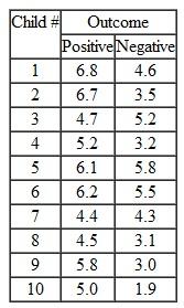
Olson, Banaji, Dweck, and Spelke (2006) read male and female children between 5-7 years old are scenarios that included positive uncontrollable outcomes for a target child (e.g., the child found $10.00 on the street) or negative uncontrollable outcomes (e.g., the child's soccer game was cancelled due to bad weather). Each child heard and number of such scenarios and rated how much he/she liked the target child on a 6-point scale where 1 = really don't like the target child and 6 = really like the target child. The mean liking rating for each set of positive and negative scenarios produced by each child was compared. Use the data shown in the table below to determine whether there was a significant difference in the median ratings given to positive vs. negative outcomes. (Note: the data shown below were created to resemble some of the data described by Olson et al.).
Olson, Banaji, Dweck, and Spelke (2006) read male and female children between 5-7 years old are scenarios that included positive uncontrollable outcomes for a target child (e.g., the child found $10.00 on the street) or negative uncontrollable outcomes (e.g., the child's soccer game was cancelled due to bad weather). Each child heard and number of such scenarios and rated how much he/she liked the target child on a 6-point scale where 1 = really don't like the target child and 6 = really like the target child. The mean liking rating for each set of positive and negative scenarios produced by each child was compared. Use the data shown in the table below to determine whether there was a significant difference in the median ratings given to positive vs. negative outcomes. (Note: the data shown below were created to resemble some of the data described by Olson et al.).
سؤال
سؤال
سؤال

فتح الحزمة
قم بالتسجيل لفتح البطاقات في هذه المجموعة!
Unlock Deck
Unlock Deck
1/6
العب
ملء الشاشة (f)
Deck 17: Nonparametric or Distribution Free Tests
1
Note: The data files named in these exercises are available at the publisher's website for this text, http://www.pearsonhighered.com/stern2e.
During 2002,.34 (i.e., 34%) of the births to teenage mothers in the U.S. were to unmarried women. To determine if this proportion differs for Americans of Japanese descent, a random sample is obtained of 112 American teenage women of Japanese descent who give birth. The number of these women who are unmarried is found to be 10. Determine if the proportion of births to unmarried teenagers of Japanese descent differs from that of the U.S. population in general in 2002.
During 2002,.34 (i.e., 34%) of the births to teenage mothers in the U.S. were to unmarried women. To determine if this proportion differs for Americans of Japanese descent, a random sample is obtained of 112 American teenage women of Japanese descent who give birth. The number of these women who are unmarried is found to be 10. Determine if the proportion of births to unmarried teenagers of Japanese descent differs from that of the U.S. population in general in 2002.
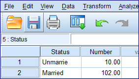
To test this question, a binomial test could be performed. Here, the number of unmarried women is 10 and the number of married women is 102. These data could be entered in the SPSS Data Editor in the following way:
 Instructions:
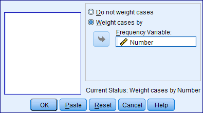
The values of the numeric variable Status would be weighted by values of the variable Number.
Go to
 Select weight cases by and specify the frequency variables (Number).
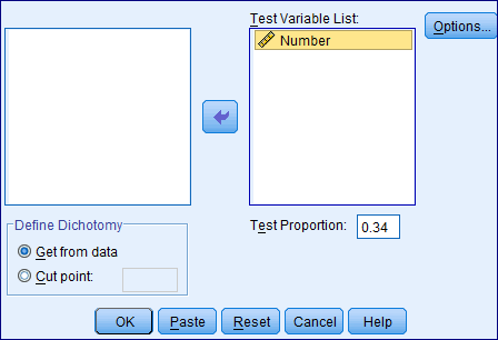
 The binomial test would be run using the test proportion is 0.34.
Under this test the null and alternative hypotheses are
 Let us assume the level of significance is
 Use Non-parametric binomial test to analyze the data.
Go to
 Specify the test variable list (Number)
Select get from data
Specify the test proportion 0.34
Click ok.
 Click on Options
Check Descriptive
Select Exclude cases test-by-test
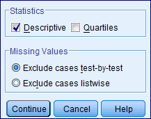 Click Continue
Then Click Ok
By following the above instructions we get the output as shown below:
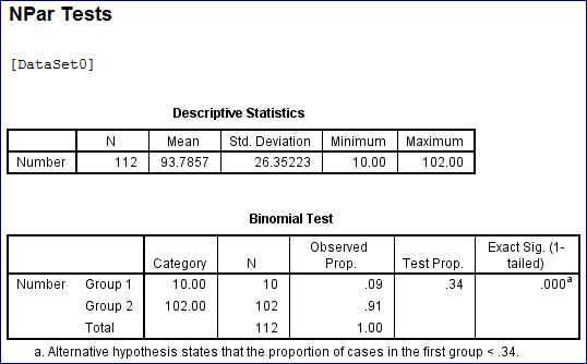 From the above output we have the calculated P -value as 0.000. Since, the value is less than 0.05 level of significance, we reject the null hypothesis and conclude that the population proportion is differ from 0.34.
Instructions:The values of the numeric variable Status would be weighted by values of the variable Number.
Go to
Select weight cases by and specify the frequency variables (Number). The binomial test would be run using the test proportion is 0.34.Under this test the null and alternative hypotheses are
Let us assume the level of significance is Use Non-parametric binomial test to analyze the data.Go to
Specify the test variable list (Number)Select get from data
Specify the test proportion 0.34
Click ok.
Click on Options Check Descriptive
Select Exclude cases test-by-test
Click Continue Then Click Ok
By following the above instructions we get the output as shown below:
From the above output we have the calculated P -value as 0.000. Since, the value is less than 0.05 level of significance, we reject the null hypothesis and conclude that the population proportion is differ from 0.34. 2
Note: The data files named in these exercises are available at the publisher's website for this text, http://www.pearsonhighered.com/stern2e.
An experimenter asks participants to read two pages of instructions for a task. Each participant's reading times are recorded in tenths of a second for each page. The file ReadtimesTwoPage.sav contains the reading time of each participant for page one in the variable time1 and for page two in the variable time2. Determine whether the median time to read pages one and two differs significantly.
An experimenter asks participants to read two pages of instructions for a task. Each participant's reading times are recorded in tenths of a second for each page. The file ReadtimesTwoPage.sav contains the reading time of each participant for page one in the variable time1 and for page two in the variable time2. Determine whether the median time to read pages one and two differs significantly.
Because the data are paired, that is, each participant provides a reading time for the first and the second page, the data may be analyzed using a Wilcoxon signed ranks test.
Under this test the null and alternative hypotheses are,
 The median time to read the two different pages is identical.
 The median times to read the two different pages are differ significantly.
Let us assume the level of significance is
 Use SPSS to test the null hypothesis and to find the test statistic value.
Instructions:
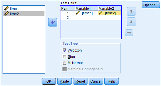
1. Go to
 And specify the Test pairs: Variable 1 ( time 1) Variable 2 (time 2).
2. Check Test Type (Wilcoxon) and click ok.
 By following the above instructions we get the output as follows:
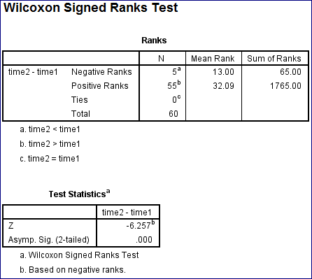 From the above output we have the test statistic value as
 And the corresponding P -value is 0.000.
Since the calculated P -value is less than the level of significance 0.05 we reject the null hypothesis and conclude that the median times to read the two different pages are differ significantly.
Under this test the null and alternative hypotheses are,
The median time to read the two different pages is identical. The median times to read the two different pages are differ significantly.Let us assume the level of significance is
Use SPSS to test the null hypothesis and to find the test statistic value.Instructions:
1. Go to
And specify the Test pairs: Variable 1 ( time 1) Variable 2 (time 2).2. Check Test Type (Wilcoxon) and click ok.
By following the above instructions we get the output as follows: From the above output we have the test statistic value as And the corresponding P -value is 0.000.Since the calculated P -value is less than the level of significance 0.05 we reject the null hypothesis and conclude that the median times to read the two different pages are differ significantly.
3
Note: The data files named in these exercises are available at the publisher's website for this text, http://www.pearsonhighered.com/stern2e.
Olson, Banaji, Dweck, and Spelke (2006) read male and female children between 5-7 years old are scenarios that included positive uncontrollable outcomes for a target child (e.g., the child found $10.00 on the street) or negative uncontrollable outcomes (e.g., the child's soccer game was cancelled due to bad weather). Each child heard and number of such scenarios and rated how much he/she liked the target child on a 6-point scale where 1 = really don't like the target child and 6 = really like the target child. The mean liking rating for each set of positive and negative scenarios produced by each child was compared. Use the data shown in the table below to determine whether there was a significant difference in the median ratings given to positive vs. negative outcomes. (Note: the data shown below were created to resemble some of the data described by Olson et al.).
Olson, Banaji, Dweck, and Spelke (2006) read male and female children between 5-7 years old are scenarios that included positive uncontrollable outcomes for a target child (e.g., the child found $10.00 on the street) or negative uncontrollable outcomes (e.g., the child's soccer game was cancelled due to bad weather). Each child heard and number of such scenarios and rated how much he/she liked the target child on a 6-point scale where 1 = really don't like the target child and 6 = really like the target child. The mean liking rating for each set of positive and negative scenarios produced by each child was compared. Use the data shown in the table below to determine whether there was a significant difference in the median ratings given to positive vs. negative outcomes. (Note: the data shown below were created to resemble some of the data described by Olson et al.).
Type the given data into the SPSS work sheet.
Perform Mann-Whitney test for the given data.
Under this test the null and alternative hypotheses are,
 The population parameters are identical.
 The population parameters are not identical.
Let us assume the level of significance is
 Use SPSS to test the null hypothesis and to find the test statistic value.
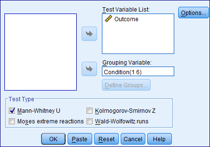
Instructions:
1. Go to
 And specify the Test variable List (Outcome) and Grouping Variable:
Condition (1, 6)
2. Check Mann-Whitney U and click Ok.
 By following the above instructions to get the output as follows:
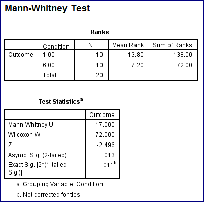 From the above output we have the test statistic value as
 And the corresponding P -value is 0.013.
Since the calculated P -value is less than the level of significance 0.05 we reject the null hypothesis and conclude that the population parameters are not identical.
Perform Mann-Whitney test for the given data.
Under this test the null and alternative hypotheses are,
The population parameters are identical. The population parameters are not identical.Let us assume the level of significance is
Use SPSS to test the null hypothesis and to find the test statistic value.Instructions:
1. Go to
And specify the Test variable List (Outcome) and Grouping Variable: Condition (1, 6)
2. Check Mann-Whitney U and click Ok.
By following the above instructions to get the output as follows: From the above output we have the test statistic value as And the corresponding P -value is 0.013.Since the calculated P -value is less than the level of significance 0.05 we reject the null hypothesis and conclude that the population parameters are not identical.
4
Note: The data files named in these exercises are available at the publisher's website for this text, http://www.pearsonhighered.com/stern2e.
Between 1944 and 2004 the proportion of Atlantic storms that were classified as hurricanes during the hurricane season (June 1-November 30) was.248. During 2005, which was an exceptional year for hurricanes, 7 storms reached hurricane strength and 20 did not. Determine if the proportion of storms that were hurricanes during 2005 differed significantly from the historical rate of.248.
Between 1944 and 2004 the proportion of Atlantic storms that were classified as hurricanes during the hurricane season (June 1-November 30) was.248. During 2005, which was an exceptional year for hurricanes, 7 storms reached hurricane strength and 20 did not. Determine if the proportion of storms that were hurricanes during 2005 differed significantly from the historical rate of.248.
فتح الحزمة
افتح القفل للوصول البطاقات البالغ عددها 6 في هذه المجموعة.
فتح الحزمة
k this deck
5
Note: The data files named in these exercises are available at the publisher's website for this text, http://www.pearsonhighered.com/stern2e.
The data file HappyMarried.sav contains data gathered by the General Social Survey given in 2004. It includes ratings of happiness measured on a scale of 1-3 where 1 = very happy, 2 = pretty happy, and 3 = not too happy. The file also identifies the marital status of each participant. Determine if the distribution of happiness ratings of married people ( marital = 1) differs from that of the never married people ( marital = 5).
The data file HappyMarried.sav contains data gathered by the General Social Survey given in 2004. It includes ratings of happiness measured on a scale of 1-3 where 1 = very happy, 2 = pretty happy, and 3 = not too happy. The file also identifies the marital status of each participant. Determine if the distribution of happiness ratings of married people ( marital = 1) differs from that of the never married people ( marital = 5).
فتح الحزمة
افتح القفل للوصول البطاقات البالغ عددها 6 في هذه المجموعة.
فتح الحزمة
k this deck
6
Note: The data files named in these exercises are available at the publisher's website for this text, http://www.pearsonhighered.com/stern2e.
Reaction time data tend to be positively skewed. The data file ReadingTimes.sav contains the reading times of participants shown one of two versions of an instruction for a laboratory task, a standard form of the instructions (labeled control ) and a new form of the instructions (labeled new ). The reading time in tenths of a second is recorded in the variable time. Conduct a test to determine whether the distributions of reading times in the two instruction conditions differ. What is the effect size, A
Reaction time data tend to be positively skewed. The data file ReadingTimes.sav contains the reading times of participants shown one of two versions of an instruction for a laboratory task, a standard form of the instructions (labeled control ) and a new form of the instructions (labeled new ). The reading time in tenths of a second is recorded in the variable time. Conduct a test to determine whether the distributions of reading times in the two instruction conditions differ. What is the effect size, A
فتح الحزمة
افتح القفل للوصول البطاقات البالغ عددها 6 في هذه المجموعة.
فتح الحزمة
k this deck
فتح الحزمة
افتح القفل للوصول البطاقات البالغ عددها 6 في هذه المجموعة.


