Deck 6: Multiple Regression Analysis: Further Issues
ملء الشاشة (f)
سؤال
Using the data in RDCHEM.RAW, the following equation was obtained by OLS: 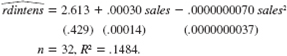
(i) At what point does the marginal effect of sales on rdintens become negative
(ii) Would you keep the quadratic term in the model Explain.
(iii) Define salesbil as sales measured in billions of dollars: salesbil _ sales/1,000. Rewrite the estimated equation with salesbil and salesbil 2 as the independent variables. Be sure to report standard errors and the R-squared.
(iv) For the purpose of reporting the results, which equation do you prefer
سؤال
سؤال
سؤال
The following model allows the return to education to depend upon the total amount of both parents' education, called pareduc: log(wage) = 0 + 1 educ + 2 educ.pareduc + 3 exper + 4 tenure + u.
(i) Show that, in decimal form, the return to another year of education in this model is log(wage)/ educ = 1 + 2 pareduc. What sign do you expect for _2 Why
(ii) Using the data in WAGE2.RAW, the estimated equation is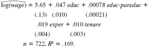
(Only 722 observations contain full information on parents' education.) Interpret the coefficient on the interaction term. It might help to choose two specific values for pareduc-for example, pareduc = 32 if both parents have a college education, or pareduc = 24 if both parents have a high school education-and to compare the estimated return to educ.
(iii) When pareduc is added as a separate variable to the equation, we get: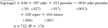 Does the estimated return to education now depend positively on parent education Test the null hypothesis that the return to education does not depend on parent education.
(i) Show that, in decimal form, the return to another year of education in this model is log(wage)/ educ = 1 + 2 pareduc. What sign do you expect for _2 Why
(ii) Using the data in WAGE2.RAW, the estimated equation is
(Only 722 observations contain full information on parents' education.) Interpret the coefficient on the interaction term. It might help to choose two specific values for pareduc-for example, pareduc = 32 if both parents have a college education, or pareduc = 24 if both parents have a high school education-and to compare the estimated return to educ.
(iii) When pareduc is added as a separate variable to the equation, we get:
Does the estimated return to education now depend positively on parent education Test the null hypothesis that the return to education does not depend on parent education. سؤال
سؤال
سؤال
سؤال
سؤال
Use the data in ATTEND.RAW for thiexercise.
(i) In the model of Example 6.3, argue that stndfnl/ priGPA 2 + 2 4 priGPA + 6 atndrte. Use equation (6.19) to estimate the partial effect when priGPA = 2.59 and atndrte = 82. Interpret your estimate.
(ii) Show that the equation can be written as stndfnl = 0 + 1 atndrte + 2 priGPA + 3ACT + 4 (priGPA - 2.59) 2 + 5 ACT 2 + 6 priGPA(atndrte - 82) + u,
where 2 = 2 + 2 4 (2.59) + 6 (82). (Note that the intercept has changed, but this is unimportant.) Use this to obtain the standard error of from part (i).
(iii) Suppose that, in place of priGPA(atndrte - 82), you put (priGPA - 2.59)-(atndrte - 82). Now how do you interpret the coefficients on atndrte and priGPA
(i) In the model of Example 6.3, argue that stndfnl/ priGPA 2 + 2 4 priGPA + 6 atndrte. Use equation (6.19) to estimate the partial effect when priGPA = 2.59 and atndrte = 82. Interpret your estimate.
(ii) Show that the equation can be written as stndfnl = 0 + 1 atndrte + 2 priGPA + 3ACT + 4 (priGPA - 2.59) 2 + 5 ACT 2 + 6 priGPA(atndrte - 82) + u,
where 2 = 2 + 2 4 (2.59) + 6 (82). (Note that the intercept has changed, but this is unimportant.) Use this to obtain the standard error of
from part (i).(iii) Suppose that, in place of priGPA(atndrte - 82), you put (priGPA - 2.59)-(atndrte - 82). Now how do you interpret the coefficients on atndrte and priGPA
سؤال
The following three equations were estimated using the 1,534 observations in 401K.RAW: 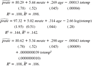
Which of these three models do you prefer Why
Which of these three models do you prefer Why
سؤال
سؤال
سؤال
سؤال
سؤال
The following equation was estimated using the data in CEOSAL1.RAW: 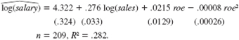 This equation allows roe to have a diminishing effect on log(salary). Is this generality necessary Explain why or why not.
This equation allows roe to have a diminishing effect on log(salary). Is this generality necessary Explain why or why not. سؤال
If we start with (6.38) under the CLM assumptions, assume large n, and ignore the esti- 
(i) For what values of _ ˆ will the point prediction be in the 95% prediction interval Does this condition seem likely to hold in most applications
(ii) Verify that the condition from part (i) is satisfied in the CEO salary example.
(i) For what values of _ ˆ will the point prediction be in the 95% prediction interval Does this condition seem likely to hold in most applications
(ii) Verify that the condition from part (i) is satisfied in the CEO salary example.
سؤال
Use the data in WAGE1.RAW for this exercise.
(i) Use OLS to estimate the equation log(wage) = 0 + 1 educ + 2 exper + 3 exper 2 + u and report the results using the usual format.
(ii) Is exper 2 statistically significant at the 1% level
(iii) Using the approximation find the approximate return to the fifth year of experience. What is the approximate return to the twentieth year of experience
(iv) At what value of exper does additional experience actually lower predicted log(wage) How many people have more experience in this sample
(i) Use OLS to estimate the equation log(wage) = 0 + 1 educ + 2 exper + 3 exper 2 + u and report the results using the usual format.
(ii) Is exper 2 statistically significant at the 1% level
(iii) Using the approximation
find the approximate return to the fifth year of experience. What is the approximate return to the twentieth year of experience (iv) At what value of exper does additional experience actually lower predicted log(wage) How many people have more experience in this sample
سؤال
سؤال
Let  be the OLS estimates from the regression of yi on x i1 , …, x ik , i_1, 2, …, n. For nonzero constants c 1 , …, c k , argue that the OLS intercept and slopes from the regres-
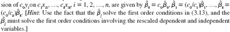
be the OLS estimates from the regression of yi on x i1 , …, x ik , i_1, 2, …, n. For nonzero constants c 1 , …, c k , argue that the OLS intercept and slopes from the regres- سؤال
سؤال
Consider a model where the return to education depends upon the amount of work experience (and vice versa): log(wage) = 0 + 1 educ + 2 exper + 3 educ + exper + u.
(i) Show that the return to another year of education (in decimal form), holding exper fixed, is 1 + 3 exper.
(ii) State the null hypothesis that the return to education does not depend on the level of exper. What do you think is the appropriate alternative
(iii) Use the data in WAGE2.RAW to test the null hypothesis in (ii) against your stated alternative.
(iv) Let _1 denote the return to education (in decimal form), when exper = 10:
1 = 1 + 10 3. Obtain and a 95% confidence interval for 1.
(i) Show that the return to another year of education (in decimal form), holding exper fixed, is 1 + 3 exper.
(ii) State the null hypothesis that the return to education does not depend on the level of exper. What do you think is the appropriate alternative
(iii) Use the data in WAGE2.RAW to test the null hypothesis in (ii) against your stated alternative.
(iv) Let _1 denote the return to education (in decimal form), when exper = 10:
1 = 1 + 10 3. Obtain
and a 95% confidence interval for 1. سؤال
Use the subset of 401KSUBS.RAW with fsize = 1; this restricts the analysis to single person households; see also Computer Exercise C4.8.
(i) What is the youngest age of people in this sample How many people are at that age
(ii) In the model
nettfa = 0 + 1 inc + 2 age + 3 age 2 + u, what is the literal interpretation of 2 By itself, is it of much interest
(iii) Estimate the model from part (ii) and report the results in standard form. Are you concerned that the coefficient on age is negative Explain.
(iv) Because the youngest people in the sample are 25, it makes sense to think that, for a given level of income, the lowest average amount of net total financial assets is at age 25. Recall that the partial effect of age on nettfa is 2 + 2 3 age, so the partial effect at age 25 is 2 + 2 3 (25) = 2 + 50 3 ; call this 2. Find and obtain the
two-sided p-value for testing H 0 : 2 = 0. You should conclude that is small and very statistically insignificant.
v) Because the evidence against H 0 : 2 = 0 is very weak, set it to zero and estimate the model nettfa = 0 + 1 inc + 3 (age - 25) 2 + u. In terms of goodness-of-fit, does this model fit better than that in part (ii)
(vi) For the estimated equation in part (v), set inc = 30 (roughly, the average value) and graph the relationship between nettfa and age, but only for age 25. Describe what you see.
(vii) Check to see whether including a quadratic in inc is necessary.
(i) What is the youngest age of people in this sample How many people are at that age
(ii) In the model
nettfa = 0 + 1 inc + 2 age + 3 age 2 + u, what is the literal interpretation of 2 By itself, is it of much interest
(iii) Estimate the model from part (ii) and report the results in standard form. Are you concerned that the coefficient on age is negative Explain.
(iv) Because the youngest people in the sample are 25, it makes sense to think that, for a given level of income, the lowest average amount of net total financial assets is at age 25. Recall that the partial effect of age on nettfa is 2 + 2 3 age, so the partial effect at age 25 is 2 + 2 3 (25) = 2 + 50 3 ; call this 2. Find
and obtain thetwo-sided p-value for testing H 0 : 2 = 0. You should conclude that
is small and very statistically insignificant.v) Because the evidence against H 0 : 2 = 0 is very weak, set it to zero and estimate the model nettfa = 0 + 1 inc + 3 (age - 25) 2 + u. In terms of goodness-of-fit, does this model fit better than that in part (ii)
(vi) For the estimated equation in part (v), set inc = 30 (roughly, the average value) and graph the relationship between nettfa and age, but only for age 25. Describe what you see.
(vii) Check to see whether including a quadratic in inc is necessary.

فتح الحزمة
قم بالتسجيل لفتح البطاقات في هذه المجموعة!
Unlock Deck
Unlock Deck
1/22
العب
ملء الشاشة (f)
Deck 6: Multiple Regression Analysis: Further Issues
1
Using the data in RDCHEM.RAW, the following equation was obtained by OLS:
(i) At what point does the marginal effect of sales on rdintens become negative
(ii) Would you keep the quadratic term in the model Explain.
(iii) Define salesbil as sales measured in billions of dollars: salesbil _ sales/1,000. Rewrite the estimated equation with salesbil and salesbil 2 as the independent variables. Be sure to report standard errors and the R-squared.
(iv) For the purpose of reporting the results, which equation do you prefer
(i)
The equation is given by: The marginal effect of
  on
on  is given by:
  For the marginal effect to be negative,
  holds
holds
This implies, Hence, at
  the marginal effect of
  on
on  become negative
(ii) The t-statistic of the coefficient of
  is given by:
  At 29 degree of freedom and 5% level of significance critical (one-tailed) t-statistic is 1.699 which is less than the actual t-statistic, indicating that the variable
  is statistically significant at 5% level of significance. This ensures that the quadratic term should be included in the model.
(iii)
Consider: Since,
  is factored by 1000, the coefficient would be multiplied by 1000 and the standard error would be divided by 1000
Hence, the model becomes: (iv)
(iv)
For the purpose of reporting, the equation that would be preferred is given by: This is because, the coefficient has less decimal places
The equation is given by:
The marginal effect of on is given by: For the marginal effect to be negative, holdsThis implies,
Hence, at the marginal effect of on become negative(ii)
The t-statistic of the coefficient of is given by: At 29 degree of freedom and 5% level of significance critical (one-tailed) t-statistic is 1.699 which is less than the actual t-statistic, indicating that the variable is statistically significant at 5% level of significance. This ensures that the quadratic term should be included in the model.(iii)
Consider:
Since, is factored by 1000, the coefficient would be multiplied by 1000 and the standard error would be divided by 1000Hence, the model becomes:
(iv)For the purpose of reporting, the equation that would be preferred is given by:
This is because, the coefficient has less decimal places 2
Use the data in MEAP00_01 to answer this question.
(i) Estimate the model math4 = 0 + 2 lexppp + 2 lenroll + 3 lunch + u by OLS, and report the results in the usual form. Is each explanatory variable statistically significant at the 5% level
(ii) Obtain the fitted values from the regression in part (i). What is the range of fitted values How does it compare with the range of the actual data on math4
(iii) Obtain the residuals from the regression in part (i). What is the building code of the school that has the largest (positive) residual Provide an interpretation of this residual.
(iv) Add quadratics of all explanatory variables to the equation, and test them for joint significance. Would you leave them in the model
(v) Returning to the model in part (i), divide the dependent variable and each explanatory variable by its sample standard deviation, and rerun the regression.(Include an intercept unless you also first subtract the mean from each variable.) In terms of standard deviation units, which explanatory variable has the largest effect on the math pass rate
NO ANSWER
3
Use the data in GPA2.RAW for this exercise.
(i) Estimate the model sat = 0 + 1 hsize + 2 hsize 2 + u, where hsize is the size of the graduating class (in hundreds), and write the results in the usual form. Is the quadratic term statistically significant
(ii) Using the estimated equation from part (i), what is the "optimal" high school size Justify your answer.
(iii) Is this analysis representative of the academic performance of all high school seniors Explain.
(iv) Find the estimated optimal high school size, using log(sat) as the dependent variable. Is it much different from what you obtained in part (ii)
(i)
The estimated equation is:![(i) The estimated equation is: The quadratic term is statistically significant, with t statistic ˜ -3.87. (ii) It is required to find the value of hsize , say hsize *, where reaches its maximum. This is the turning point in the parabola, which hsize * comes out to be 19.81/ [2(2.13)] 4.65. Since hsize is in 100s, this means 465 students is the optimal class size. Of course, the very small R -squared shows that class size explains only a tiny amount of the variation in SAT score. (iii) Only students who actually take the SAT exam appear in the sample, so it is not representative of all high school seniors. If the population of interest is all high school seniors, a random sample of such students who all took the same standardized exam will be needed. (iv) With log( sat ) as the dependent variable, the equation becomes: The optimal class size is now estimated as about 469, which is very close to what was obtained with the level-level model.](https://d2lvgg3v3hfg70.cloudfront.net/SM2712/11eb9ee2_f0a1_dfcf_8edd_dd458f65e473_SM2712_00.jpg) The quadratic term is statistically significant, with t statistic ˜ -3.87.
The quadratic term is statistically significant, with t statistic ˜ -3.87.
(ii)
It is required to find the value of hsize , say hsize *, where reaches its maximum. This is the turning point in the parabola, which hsize * comes out to be 19.81/ [2(2.13)] 4.65. Since hsize is in 100s, this means 465 students is the "optimal" class size.
Of course, the very small R -squared shows that class size explains only a tiny amount of the variation in SAT score.
(iii)
Only students who actually take the SAT exam appear in the sample, so it is not representative of all high school seniors. If the population of interest is all high school seniors, a random sample of such students who all took the same standardized exam will be needed.
(iv)
With log( sat ) as the dependent variable, the equation becomes:![(i) The estimated equation is: The quadratic term is statistically significant, with t statistic ˜ -3.87. (ii) It is required to find the value of hsize , say hsize *, where reaches its maximum. This is the turning point in the parabola, which hsize * comes out to be 19.81/ [2(2.13)] 4.65. Since hsize is in 100s, this means 465 students is the optimal class size. Of course, the very small R -squared shows that class size explains only a tiny amount of the variation in SAT score. (iii) Only students who actually take the SAT exam appear in the sample, so it is not representative of all high school seniors. If the population of interest is all high school seniors, a random sample of such students who all took the same standardized exam will be needed. (iv) With log( sat ) as the dependent variable, the equation becomes: The optimal class size is now estimated as about 469, which is very close to what was obtained with the level-level model.](https://d2lvgg3v3hfg70.cloudfront.net/SM2712/11eb9ee2_f0a1_dfd0_8edd_6b898933a481_SM2712_00.jpg) The optimal class size is now estimated as about 469, which is very close to what was obtained with the level-level model.
The optimal class size is now estimated as about 469, which is very close to what was obtained with the level-level model.
The estimated equation is:
The quadratic term is statistically significant, with t statistic ˜ -3.87.(ii)
It is required to find the value of hsize , say hsize *, where reaches its maximum. This is the turning point in the parabola, which hsize * comes out to be 19.81/ [2(2.13)] 4.65. Since hsize is in 100s, this means 465 students is the "optimal" class size.
Of course, the very small R -squared shows that class size explains only a tiny amount of the variation in SAT score.
(iii)
Only students who actually take the SAT exam appear in the sample, so it is not representative of all high school seniors. If the population of interest is all high school seniors, a random sample of such students who all took the same standardized exam will be needed.
(iv)
With log( sat ) as the dependent variable, the equation becomes:
The optimal class size is now estimated as about 469, which is very close to what was obtained with the level-level model. 4
The following model allows the return to education to depend upon the total amount of both parents' education, called pareduc: log(wage) = 0 + 1 educ + 2 educ.pareduc + 3 exper + 4 tenure + u.
(i) Show that, in decimal form, the return to another year of education in this model is log(wage)/ educ = 1 + 2 pareduc. What sign do you expect for _2 Why
(ii) Using the data in WAGE2.RAW, the estimated equation is
(Only 722 observations contain full information on parents' education.) Interpret the coefficient on the interaction term. It might help to choose two specific values for pareduc-for example, pareduc = 32 if both parents have a college education, or pareduc = 24 if both parents have a high school education-and to compare the estimated return to educ.
(iii) When pareduc is added as a separate variable to the equation, we get: Does the estimated return to education now depend positively on parent education Test the null hypothesis that the return to education does not depend on parent education.
(i) Show that, in decimal form, the return to another year of education in this model is log(wage)/ educ = 1 + 2 pareduc. What sign do you expect for _2 Why
(ii) Using the data in WAGE2.RAW, the estimated equation is
(Only 722 observations contain full information on parents' education.) Interpret the coefficient on the interaction term. It might help to choose two specific values for pareduc-for example, pareduc = 32 if both parents have a college education, or pareduc = 24 if both parents have a high school education-and to compare the estimated return to educ.
(iii) When pareduc is added as a separate variable to the equation, we get:
Does the estimated return to education now depend positively on parent education Test the null hypothesis that the return to education does not depend on parent education. فتح الحزمة
افتح القفل للوصول البطاقات البالغ عددها 22 في هذه المجموعة.
فتح الحزمة
k this deck
5
Use the housing price data in HPRICE1.RAW for this exercise.
(i) Estimate the model log(price) + 0 + 1 log(lotsize) + 2 log(sqrft) + 3 bdrms = u and report the results in the usual OLS format. 220 Part 1 Regression Analysis with Cross-Sectional Data
(ii) Find the predicted value of log(price), when lotsize = 20,000, sqrft = 2,500, and bdrms = 4. Using the methods in Section 6.4, find the predicted value of price at the same values of the explanatory variables.
(iii) For explaining variation in price, decide whether you prefer the model from part (i) or the model
price = 0 + 1 lotsize + 2 sqrft + 3 bdrms + u.
فتح الحزمة
افتح القفل للوصول البطاقات البالغ عددها 22 في هذه المجموعة.
فتح الحزمة
k this deck
6
In Example 4.2, where the percentage of students receiving a passing score on a tenth-grade math exam (math10) is the dependent variable, does it make sense to include sci11-the percentage of eleventh graders passing a science exam-as an additional explanatory variable
فتح الحزمة
افتح القفل للوصول البطاقات البالغ عددها 22 في هذه المجموعة.
فتح الحزمة
k this deck
7
Use the data in VOTE1.RAW for this exercise.
(i) Consider a model with an interaction between expenditures: voteA = 0 + 1 prtystrA + 2 expendA + 3 expendB + 4 expendA.expendB + u. What is the partial effect of expendB on voteA, holding prtystrA and expendA fixed What is the partial effect of expendA on voteA Is the expected sign for 4 obvious
(ii) Estimate the equation in part (i) and report the results in the usual form. Is the interaction term statistically significant
(iii) Find the average of expendA in the sample. Fix expendA at 300 (for $300,000).
What is the estimated effect of another $100,000 spent by Candidate B on voteA Is this a large effect
(iv) Now fix expendB at 100. What is the estimated effect of expendA = 100 on voteA Does this make sense
(v) Now, estimate a model that replaces the interaction with shareA, Candidate A's percentage share of total campaign expenditures. Does it make sense to hold both expendA and expendB fixed, while changing shareA
(vi) (Requires calculus) In the model from part (v), find the partial effect of expend on voteA, holding prtystrA and expendA fixed. Evaluate this at expendA = 300 and expendB = 0 and comment on the results.
فتح الحزمة
افتح القفل للوصول البطاقات البالغ عددها 22 في هذه المجموعة.
فتح الحزمة
k this deck
8
When atndrte2 and ACT_atndrte are added to the equation estimated in (6.19), the R-squared becomes.232. Are these additional terms jointly significant at the 10% level Would you include them in the model
فتح الحزمة
افتح القفل للوصول البطاقات البالغ عددها 22 في هذه المجموعة.
فتح الحزمة
k this deck
9
Use the data in ATTEND.RAW for thiexercise.
(i) In the model of Example 6.3, argue that stndfnl/ priGPA 2 + 2 4 priGPA + 6 atndrte. Use equation (6.19) to estimate the partial effect when priGPA = 2.59 and atndrte = 82. Interpret your estimate.
(ii) Show that the equation can be written as stndfnl = 0 + 1 atndrte + 2 priGPA + 3ACT + 4 (priGPA - 2.59) 2 + 5 ACT 2 + 6 priGPA(atndrte - 82) + u,
where 2 = 2 + 2 4 (2.59) + 6 (82). (Note that the intercept has changed, but this is unimportant.) Use this to obtain the standard error of from part (i).
(iii) Suppose that, in place of priGPA(atndrte - 82), you put (priGPA - 2.59)-(atndrte - 82). Now how do you interpret the coefficients on atndrte and priGPA
(i) In the model of Example 6.3, argue that stndfnl/ priGPA 2 + 2 4 priGPA + 6 atndrte. Use equation (6.19) to estimate the partial effect when priGPA = 2.59 and atndrte = 82. Interpret your estimate.
(ii) Show that the equation can be written as stndfnl = 0 + 1 atndrte + 2 priGPA + 3ACT + 4 (priGPA - 2.59) 2 + 5 ACT 2 + 6 priGPA(atndrte - 82) + u,
where 2 = 2 + 2 4 (2.59) + 6 (82). (Note that the intercept has changed, but this is unimportant.) Use this to obtain the standard error of
from part (i).(iii) Suppose that, in place of priGPA(atndrte - 82), you put (priGPA - 2.59)-(atndrte - 82). Now how do you interpret the coefficients on atndrte and priGPA
فتح الحزمة
افتح القفل للوصول البطاقات البالغ عددها 22 في هذه المجموعة.
فتح الحزمة
k this deck
10
The following three equations were estimated using the 1,534 observations in 401K.RAW:
Which of these three models do you prefer Why
Which of these three models do you prefer Why
فتح الحزمة
افتح القفل للوصول البطاقات البالغ عددها 22 في هذه المجموعة.
فتح الحزمة
k this deck
11
Use the data in HPRICE1.RAW for this exercise.
(i) Estimate the model
price = 0 + 1 lotsize + 2 sqrft + 3 bdrms + u
and report the results in the usual form, including the standard error of the regression. Obtain predicted price, when we plug in lotsize = 10,000, sqrft = 2,300, and bdrms = 4; round this price to the nearest dollar.
(ii) Run a regression that allows you to put a 95% confidence interval around the predicted value in part (i). Note that your prediction will differ somewhat due to rounding error.
(iii) Let price0 be the unknown future selling price of the house with the characteristicsused in parts (i) and (ii). Find a 95% CI for price 0 and comment on the width of this confidence interval.
فتح الحزمة
افتح القفل للوصول البطاقات البالغ عددها 22 في هذه المجموعة.
فتح الحزمة
k this deck
12
Suppose we want to estimate the effects of alcohol consumption (alcohol) on college grade point average (colGPA). In addition to collecting information on grade point averages and alcohol usage, we also obtain attendance information (say, percentage of lectures attended, called attend). A standardized test score (say, SAT) and high school GPA (hsGPA) are also available.
(i) Should we include attend along with alcohol as explanatory variables in a multiple regression model (Think about how you would interpret alcohol.)
(ii) Should SAT and hsGPA be included as explanatory variables Explain.
(i) Should we include attend along with alcohol as explanatory variables in a multiple regression model (Think about how you would interpret alcohol.)
(ii) Should SAT and hsGPA be included as explanatory variables Explain.
فتح الحزمة
افتح القفل للوصول البطاقات البالغ عددها 22 في هذه المجموعة.
فتح الحزمة
k this deck
13
Use the data in KIELMC.RAW, only for the year 1981, to answer the following questions. The data are for houses that sold during 1981 in North Andover, Massachusetts; 1981 was the year construction began on a local garbage incinerator.
(i) To study the effects of the incinerator location on housing price, consider the simple regression model log(price) = 0 + 1 log(dist) + u, where price is housing price in dollars and dist is distance from the house to the incinerator measured in feet. Interpreting this equation causally, what sign do you expect for 1 if the presence of the incinerator depresses housing prices Estimate this equation and interpret the results.
(ii) To the simple regression model in part (i), add the variables log(intst), log(area), log(land), rooms, baths, and age, where intst is distance from the home to the interstate, area is square footage of the house, land is the lot size in square feet, rooms is total number of rooms, baths is number of bathrooms, and age is age of the house in years. Now, what do you conclude about the effects of the incinerator Explain why (i) and (ii) give conflicting results.
(iii) Add [log(intst)]2to the model from part (ii). Now what happens What do you conclude about the importance of functional form
(iv) Is the square of log(dist) significant when you add it to the model from part (iii) .
فتح الحزمة
افتح القفل للوصول البطاقات البالغ عددها 22 في هذه المجموعة.
فتح الحزمة
k this deck
14
The data set NBASAL.RAW contains salary information and career statistics for 269 players in the National Basketball Association (NBA).
(i) Estimate a model relating points-per-game (points) to years in the league (exper),age, and years played in college (coll). Include a quadratic in exper; the other variables should appear in level form. Report the results in the usual way.
(ii) Holding college years and age fixed, at what value of experience does the next year of experience actually reduce points-per-game Does this make sense
(iii) Why do you think coll has a negative and statistically significant coefficient
(iv) Add a quadratic in age to the equation. Is it needed What does this appear to imply about the effects of age, once experience and education are controlled for
(v) Now regress log(wage) on points, exper, exper 2 , age, and coll. Report the results in the usual format.
(vi) Test whether age and coll are jointly significant in the regression from part (v).What does this imply about whether age and education have separate effects on wage, once productivity and seniority are accounted for
فتح الحزمة
افتح القفل للوصول البطاقات البالغ عددها 22 في هذه المجموعة.
فتح الحزمة
k this deck
15
The following equation was estimated using the data in CEOSAL1.RAW: This equation allows roe to have a diminishing effect on log(salary). Is this generality necessary Explain why or why not.
This equation allows roe to have a diminishing effect on log(salary). Is this generality necessary Explain why or why not. فتح الحزمة
افتح القفل للوصول البطاقات البالغ عددها 22 في هذه المجموعة.
فتح الحزمة
k this deck
16
If we start with (6.38) under the CLM assumptions, assume large n, and ignore the esti-
(i) For what values of _ ˆ will the point prediction be in the 95% prediction interval Does this condition seem likely to hold in most applications
(ii) Verify that the condition from part (i) is satisfied in the CEO salary example.
(i) For what values of _ ˆ will the point prediction be in the 95% prediction interval Does this condition seem likely to hold in most applications
(ii) Verify that the condition from part (i) is satisfied in the CEO salary example.
فتح الحزمة
افتح القفل للوصول البطاقات البالغ عددها 22 في هذه المجموعة.
فتح الحزمة
k this deck
17
Use the data in WAGE1.RAW for this exercise.
(i) Use OLS to estimate the equation log(wage) = 0 + 1 educ + 2 exper + 3 exper 2 + u and report the results using the usual format.
(ii) Is exper 2 statistically significant at the 1% level
(iii) Using the approximation find the approximate return to the fifth year of experience. What is the approximate return to the twentieth year of experience
(iv) At what value of exper does additional experience actually lower predicted log(wage) How many people have more experience in this sample
(i) Use OLS to estimate the equation log(wage) = 0 + 1 educ + 2 exper + 3 exper 2 + u and report the results using the usual format.
(ii) Is exper 2 statistically significant at the 1% level
(iii) Using the approximation
find the approximate return to the fifth year of experience. What is the approximate return to the twentieth year of experience (iv) At what value of exper does additional experience actually lower predicted log(wage) How many people have more experience in this sample
فتح الحزمة
افتح القفل للوصول البطاقات البالغ عددها 22 في هذه المجموعة.
فتح الحزمة
k this deck
18
Use the data in BWGHT2.RAW for this exercise.
(i) Estimate the equation
log(bwght) = 0 + 1 npvis + 2 npvis 2 + u by OLS, and report the results in the usual way. Is the quadratic term significant
(ii) Show that, based on the equation from part (i), the number of prenatal visits that maximizes log(bwght) is estimated to be about 22. How many women had at least 22 prenatal visits in the sample
(iii) Does it make sense that birth weight is actually predicted to decline after 22 prenatal visits Explain.
(iv) Add mother's age to the equation, using a quadratic functional form. Holding npvis fixed, at what mother's age is the birth weight of the child maximized What fraction of women in the sample are older than the "optimal" age
(v) Would you say that mother's age and number of prenatal visits explain a lot of the variation in log(bwght)
(vi) Using quadratics for both npvis and age, decide whether using the natural log or the level of bwght is better for predicting bwght.
فتح الحزمة
افتح القفل للوصول البطاقات البالغ عددها 22 في هذه المجموعة.
فتح الحزمة
k this deck
19
Let be the OLS estimates from the regression of yi on x i1 , …, x ik , i_1, 2, …, n. For nonzero constants c 1 , …, c k , argue that the OLS intercept and slopes from the regres-
be the OLS estimates from the regression of yi on x i1 , …, x ik , i_1, 2, …, n. For nonzero constants c 1 , …, c k , argue that the OLS intercept and slopes from the regres- فتح الحزمة
افتح القفل للوصول البطاقات البالغ عددها 22 في هذه المجموعة.
فتح الحزمة
k this deck
20
Use APPLE.RAW to verify some of the claims made in Section 6.3.
(i) Run the regression ecolbs on ecoprc, regprc and report the results in the usual form, including the R-squared and adjusted R-squared. Interpret the coefficients on the price variables and comment on their signs and magnitudes.
(ii) Are the price variables statistically significant Report the p-values for the individual t tests.
(iii) What is the range of fitted values for ecolbs What fraction of the sample reports ecolbs = 0 Comment.
(iv) Do you think the price variables together do a good job of explaining variation in ecolbs Explain.
(v) Add the variables faminc, hhsize (household size), educ, and age to the regression from part (i). Find the p-value for their joint significance. What do you conclude
فتح الحزمة
افتح القفل للوصول البطاقات البالغ عددها 22 في هذه المجموعة.
فتح الحزمة
k this deck
21
Consider a model where the return to education depends upon the amount of work experience (and vice versa): log(wage) = 0 + 1 educ + 2 exper + 3 educ + exper + u.
(i) Show that the return to another year of education (in decimal form), holding exper fixed, is 1 + 3 exper.
(ii) State the null hypothesis that the return to education does not depend on the level of exper. What do you think is the appropriate alternative
(iii) Use the data in WAGE2.RAW to test the null hypothesis in (ii) against your stated alternative.
(iv) Let _1 denote the return to education (in decimal form), when exper = 10:
1 = 1 + 10 3. Obtain and a 95% confidence interval for 1.
(i) Show that the return to another year of education (in decimal form), holding exper fixed, is 1 + 3 exper.
(ii) State the null hypothesis that the return to education does not depend on the level of exper. What do you think is the appropriate alternative
(iii) Use the data in WAGE2.RAW to test the null hypothesis in (ii) against your stated alternative.
(iv) Let _1 denote the return to education (in decimal form), when exper = 10:
1 = 1 + 10 3. Obtain
and a 95% confidence interval for 1. فتح الحزمة
افتح القفل للوصول البطاقات البالغ عددها 22 في هذه المجموعة.
فتح الحزمة
k this deck
22
Use the subset of 401KSUBS.RAW with fsize = 1; this restricts the analysis to single person households; see also Computer Exercise C4.8.
(i) What is the youngest age of people in this sample How many people are at that age
(ii) In the model
nettfa = 0 + 1 inc + 2 age + 3 age 2 + u, what is the literal interpretation of 2 By itself, is it of much interest
(iii) Estimate the model from part (ii) and report the results in standard form. Are you concerned that the coefficient on age is negative Explain.
(iv) Because the youngest people in the sample are 25, it makes sense to think that, for a given level of income, the lowest average amount of net total financial assets is at age 25. Recall that the partial effect of age on nettfa is 2 + 2 3 age, so the partial effect at age 25 is 2 + 2 3 (25) = 2 + 50 3 ; call this 2. Find and obtain the
two-sided p-value for testing H 0 : 2 = 0. You should conclude that is small and very statistically insignificant.
v) Because the evidence against H 0 : 2 = 0 is very weak, set it to zero and estimate the model nettfa = 0 + 1 inc + 3 (age - 25) 2 + u. In terms of goodness-of-fit, does this model fit better than that in part (ii)
(vi) For the estimated equation in part (v), set inc = 30 (roughly, the average value) and graph the relationship between nettfa and age, but only for age 25. Describe what you see.
(vii) Check to see whether including a quadratic in inc is necessary.
(i) What is the youngest age of people in this sample How many people are at that age
(ii) In the model
nettfa = 0 + 1 inc + 2 age + 3 age 2 + u, what is the literal interpretation of 2 By itself, is it of much interest
(iii) Estimate the model from part (ii) and report the results in standard form. Are you concerned that the coefficient on age is negative Explain.
(iv) Because the youngest people in the sample are 25, it makes sense to think that, for a given level of income, the lowest average amount of net total financial assets is at age 25. Recall that the partial effect of age on nettfa is 2 + 2 3 age, so the partial effect at age 25 is 2 + 2 3 (25) = 2 + 50 3 ; call this 2. Find
and obtain thetwo-sided p-value for testing H 0 : 2 = 0. You should conclude that
is small and very statistically insignificant.v) Because the evidence against H 0 : 2 = 0 is very weak, set it to zero and estimate the model nettfa = 0 + 1 inc + 3 (age - 25) 2 + u. In terms of goodness-of-fit, does this model fit better than that in part (ii)
(vi) For the estimated equation in part (v), set inc = 30 (roughly, the average value) and graph the relationship between nettfa and age, but only for age 25. Describe what you see.
(vii) Check to see whether including a quadratic in inc is necessary.
فتح الحزمة
افتح القفل للوصول البطاقات البالغ عددها 22 في هذه المجموعة.
فتح الحزمة
k this deck
فتح الحزمة
افتح القفل للوصول البطاقات البالغ عددها 22 في هذه المجموعة.


