Deck 3: Residual Statistics
ملء الشاشة (f)
سؤال
سؤال
سؤال
سؤال
سؤال

فتح الحزمة
قم بالتسجيل لفتح البطاقات في هذه المجموعة!
Unlock Deck
Unlock Deck
1/5
العب
ملء الشاشة (f)
Deck 3: Residual Statistics
1
Given: (6 pts. each)
Dependent Variable: LNWAGES
Method: Least Squares
Date: 12/05/08 Time: 10:01
Sample: 1534
Included observations: 534
Where: LNWAGES = the natural log of pay per hour of work
ED = years of education
FEM = 1 if female, 0 otherwise
A) Interpret the value of the constant term.
B) Interpret the value of the coefficient on ED.
C) Interpret the value of the coefficient on FEM.
D) According to this model, what are the expected wages of a female with 16 years of education?
A) If ED=FEM=0, then LNWAGES=1.17 (WAGES=3.21).
B) If ED increases 1 unit, then WAGES is expected to increase 7.69%
C) A female's wages are expected to be 23.21% lower than a male's holding ED constant.
D) 8.69
B) If ED increases 1 unit, then WAGES is expected to increase 7.69%
C) A female's wages are expected to be 23.21% lower than a male's holding ED constant.
D) 8.69
2
Given: (7 pts. each)
Dependent Variable: WAGES
Method: Least Squares
Date: 12/08/08 Time: 10:39
Sample: 1534
Included observations: 534
Where:WAGES = pay per hour of work
EXPER = years of experience
FEM = 1 if female, 0 otherwise
CHICKt-2 + et "
A) Interpret the coefficient on EXPER.
B) Interpret the coefficient on EXPER*FEM.
C) Draw a diagram reflecting the regression results with WAGES on the vertical axis and
EXPER on the horizontal axis. Label all intercepts and slopes.
D) What would be the new values of the structural parameters if the dummy was flip-flopped?
E) Which regression fits better, the one from question 1 or the one from question 2? Explain.
A) If a male attaines an extra year of EXP, then wages are expected to increase .081 units.
B) If a female gains an extra year of EXP, then wages are expected to increase .080 less than a male's wages would.
C)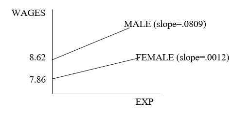 D) WAGES = 7.85704 +.001152 EXPER + .7651 FEM + .079757 INTER
E) It is impossible to tell since the dependent variables differ.
B) If a female gains an extra year of EXP, then wages are expected to increase .080 less than a male's wages would.
C)
D) WAGES = 7.85704 +.001152 EXPER + .7651 FEM + .079757 INTERE) It is impossible to tell since the dependent variables differ.
3
Given: (7 pts. each)
Dependent Variable:
Method: Least Squares
Sample(adjusted): 1695
Included observations: 695 after adjusting endpoints
Where: BINGE = 1 if student is a binge drinker, 0 otherwise
GPA = grade point average
MALE = 1 if male, 0 otherwise
WHITE = 1 if white, 0 otherwise
A) Interpret the constant term.
B) Interpret the coefficient on GPA.
C) Interpret the coefficient on MALE.
D) According to this model, what is the probability that a white female with a 2.8 GPA is a binge drinker?
A) A nonwhite female with 0 GPA is has an 81.86% of being a binge drinker.
B) If a GPA increases 1 unit, the probability of binging decreases 12.57%.
C) A male is 13.56% more likely to binge than a female holding GPA constant regardless of race.
D) 66.68%
B) If a GPA increases 1 unit, the probability of binging decreases 12.57%.
C) A male is 13.56% more likely to binge than a female holding GPA constant regardless of race.
D) 66.68%
4
Given: (4 pts.)
Dependent Variable:
Method: ML - Birary Logit (Quadratic hill climbing)
Sample(adjusted): 1695
Included observations: 695 after adjusting endpoints
Convergence achieved after 4 iterations
Covariance matrix computed using second derivatives
What is the probability that a male with a GPA = 2.8 is a binge drinker? Show your calculations.
فتح الحزمة
افتح القفل للوصول البطاقات البالغ عددها 5 في هذه المجموعة.
فتح الحزمة
k this deck
5
Suppose you are estimating an equation to predict daily changes in the Dow Jones Industrial Average over the past 5 years (so you have 1250 observations.) In addition to a bunch of other explanatory variables, you decided to include a dummy variable (ODDDAY = 1 on an odd numbered day (i.e. the 25th of the month, as opposed to the 26th); zero otherwise) to capture whether or not the day was odd numbered. Your hypothesis is that people psychologically prefer even numbers, so the DJIA should move higher on even number days and lower on odd number days.
Your results look like this = -12.87 + ……. - 7.92 ODDDAY
(-4.65) (-2.1)
(where …… represents results on all the rest of the X variables and t-statistics are in parentheses)
A) The results shown can be taken to mean that you were right: the negative feelings about odd days cause people to react negatively in the stock market, and those negative odd-day feelings cause the DJIA fall. True, false, or uncertain? Explain.
B) What would be a good guess for the value of the p-value on the coefficient attached to ODDDAY? Explain.
C) When you drop ODDDAY from the model R2 decreases a small amount; adjusted R2 decreases a small amount; and the Akaike Information Criterion falls a small amount. Explain what these three changes imply about whether ODDDAY belongs in the model or not.
D) A classmate says your model must be bad because the estimated intercept coefficient of
-12.87 makes no sense-the DJIA cannot be negative. How do you respond?
فتح الحزمة
افتح القفل للوصول البطاقات البالغ عددها 5 في هذه المجموعة.
فتح الحزمة
k this deck
فتح الحزمة
افتح القفل للوصول البطاقات البالغ عددها 5 في هذه المجموعة.


