Deck 14: Introduction to Time Series Regression and Forecasting
ملء الشاشة (f)
سؤال
سؤال
سؤال
سؤال
سؤال
سؤال
سؤال
سؤال
سؤال
سؤال
سؤال
سؤال
سؤال
سؤال
سؤال
سؤال
سؤال
سؤال
سؤال
سؤال
سؤال
سؤال
سؤال
سؤال
The textbook displayed the accompanying four economic time series with "markedly different patterns." For each indicate what you think the sample autocorrelations of the level (Y)and change (△Y)will be and explain your reasoning.
(a)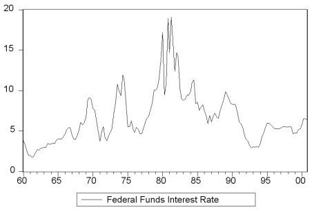 (b)
(b) 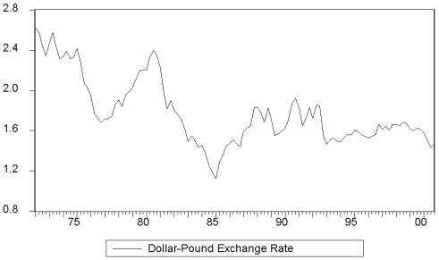 (c)
(c) 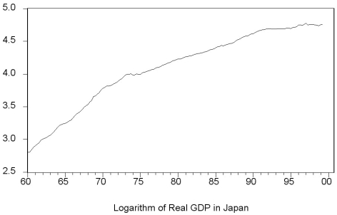 (d)
(d) 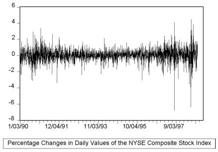
(a)
(b) (c) (d) سؤال
سؤال
There is some evidence that the Phillips curve has been unstable during the 1962 to 1999 period for the United States, and in particular during the 1990s. You set out to investigate whether or not this instability also occurred in other places. Canada is a particularly interesting case, due to its proximity to the United States and the fact that many features of its economy are similar to that of the U.S.
(a)Reading up on some of the comparative economic performance literature, you find that Canadian unemployment rates were roughly the same as U.S. unemployment rates from the 1920s to the early 1980s. The accompanying figure shows that a gap opened between the unemployment rates of the two countries in 1982, which has persisted to this date.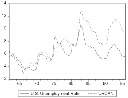 Inspection of the graph and data suggest that the break occurred during the second quarter of 1982. To investigate whether the Canadian Phillips curve shows a break at that point, you estimate an ADL(4,4)model for the sample period 1962:I-1999:IV and perform a Chow test. Specifically you postulate that the constant and coefficients of the unemployment rates changed at that point. The F-statistic is 1.96. Find the critical value from the F-table and test the null hypothesis that a break occurred at that time. Is there any reason why you should be skeptical about the result regarding the break and using the Chow-test to detect it?
(b)You consider alternative ways to test for a break in the relationship. The accompanying figure shows the F-statistics testing for a break in the ADL(4,4)equation at different dates.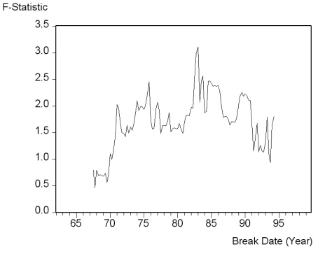 The QLR-statistic with 15% trimming is 3.11. Comment on the figure and test for the hypothesis of a break in the ADL(4,4)regression.
(c)To test for the stability of the Canadian Phillips curve in the 1990s, you decide to perform a pseudo out-of-sample forecasting. For the 24 quarters from 1994:I-1999:IV you use the ADL(4,4)model to calculate the forecasted change in the inflation rate, the resulting forecasted inflation rate, and the forecast error. The standard error of the ADL(4,4)for the estimation sample period 1962:1-1993:4 is 1.91 and the sample RMSFE is 1.70. The average forecast error for the 24 inflation rates is 0.003 and the sample standard deviation of the forecast errors is 0.82. Calculate the t-statistic and test the hypothesis that the mean out-of-sample forecast error is zero. Comment on the result and the accompanying figure of the actual and forecasted inflation rate.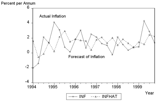
(a)Reading up on some of the comparative economic performance literature, you find that Canadian unemployment rates were roughly the same as U.S. unemployment rates from the 1920s to the early 1980s. The accompanying figure shows that a gap opened between the unemployment rates of the two countries in 1982, which has persisted to this date.
Inspection of the graph and data suggest that the break occurred during the second quarter of 1982. To investigate whether the Canadian Phillips curve shows a break at that point, you estimate an ADL(4,4)model for the sample period 1962:I-1999:IV and perform a Chow test. Specifically you postulate that the constant and coefficients of the unemployment rates changed at that point. The F-statistic is 1.96. Find the critical value from the F-table and test the null hypothesis that a break occurred at that time. Is there any reason why you should be skeptical about the result regarding the break and using the Chow-test to detect it?(b)You consider alternative ways to test for a break in the relationship. The accompanying figure shows the F-statistics testing for a break in the ADL(4,4)equation at different dates.
The QLR-statistic with 15% trimming is 3.11. Comment on the figure and test for the hypothesis of a break in the ADL(4,4)regression.(c)To test for the stability of the Canadian Phillips curve in the 1990s, you decide to perform a pseudo out-of-sample forecasting. For the 24 quarters from 1994:I-1999:IV you use the ADL(4,4)model to calculate the forecasted change in the inflation rate, the resulting forecasted inflation rate, and the forecast error. The standard error of the ADL(4,4)for the estimation sample period 1962:1-1993:4 is 1.91 and the sample RMSFE is 1.70. The average forecast error for the 24 inflation rates is 0.003 and the sample standard deviation of the forecast errors is 0.82. Calculate the t-statistic and test the hypothesis that the mean out-of-sample forecast error is zero. Comment on the result and the accompanying figure of the actual and forecasted inflation rate.
سؤال
سؤال
You collect monthly data on the money supply (M2)for the United States from 1962:1-2002:4 to forecast future money supply behavior. 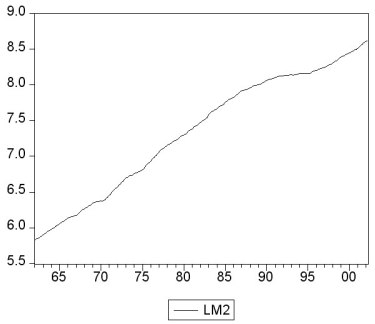
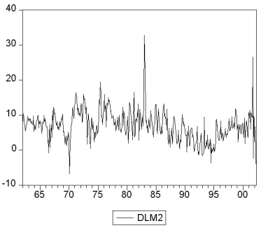 where LM2 and DLM2 are the log level and growth rate of M2.
(a)Using quarterly data, when analyzing inflation and unemployment in the United States, the textbook converted log levels of variables into growth rates by differencing the log levels, and then multiplying these by 400. Given that you have monthly data, how would you proceed here?
(b)How would you go about testing for a stochastic trend in LM2 and DLM2? Be specific about how to decide the number of lags to be included and whether or not to include a deterministic trend in your test. The textbook found the (quarterly)inflation rate to have a unit root. Does this have any affect on your expectation about whether or not the (monthly)money growth rate should be stationary?
(c)You decide to conduct an ADF unit root test for LM2, DLM2, and the change in the growth rate ΔDLM2. This results in the following t-statistic on the parameter of interest.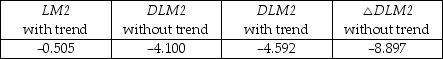 Find the critical value at the 1%, 5%, and 10% level and decide which of the coefficients is significant. What is the alternative hypothesis?
(d)In forecasting the money growth rate, you add lags of the monetary base growth rate (DLMB)to see if you can improve on the forecasting performance of a chosen AR(10)model in DLM2. You perform a Granger causality test on the 9 lags of DLMB and find a F-statistic of 2.31. Discuss the implications.
(e)Curious about the result in the previous question, you decide to estimate an ADL(10,10)for DLMB and calculate the F-statistic for the Granger causality test on the 9 lag coefficients of DLM2. This turns out to be 0.66. Discuss.
(f)Is there any a priori reason for you to be skeptical of the results? What other tests should you perform?
where LM2 and DLM2 are the log level and growth rate of M2.(a)Using quarterly data, when analyzing inflation and unemployment in the United States, the textbook converted log levels of variables into growth rates by differencing the log levels, and then multiplying these by 400. Given that you have monthly data, how would you proceed here?
(b)How would you go about testing for a stochastic trend in LM2 and DLM2? Be specific about how to decide the number of lags to be included and whether or not to include a deterministic trend in your test. The textbook found the (quarterly)inflation rate to have a unit root. Does this have any affect on your expectation about whether or not the (monthly)money growth rate should be stationary?
(c)You decide to conduct an ADF unit root test for LM2, DLM2, and the change in the growth rate ΔDLM2. This results in the following t-statistic on the parameter of interest.
Find the critical value at the 1%, 5%, and 10% level and decide which of the coefficients is significant. What is the alternative hypothesis?(d)In forecasting the money growth rate, you add lags of the monetary base growth rate (DLMB)to see if you can improve on the forecasting performance of a chosen AR(10)model in DLM2. You perform a Granger causality test on the 9 lags of DLMB and find a F-statistic of 2.31. Discuss the implications.
(e)Curious about the result in the previous question, you decide to estimate an ADL(10,10)for DLMB and calculate the F-statistic for the Granger causality test on the 9 lag coefficients of DLM2. This turns out to be 0.66. Discuss.
(f)Is there any a priori reason for you to be skeptical of the results? What other tests should you perform?
سؤال
سؤال
You set out to forecast the unemployment rate in the United States (UrateUS), using quarterly data from 1960, first quarter, to 1999, fourth quarter.
(a)The following table presents the first four autocorrelations for the United States aggregate unemployment rate and its change for the time period 1960 (first quarter)to 1999 (fourth quarter). Explain briefly what these two autocorrelations measure.
First Four Autocorrelations of the U.S. Unemployment Rate and Its Change,
1960:I - 1999:IV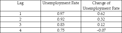 (b)The accompanying table gives changes in the United States aggregate unemployment rate for the period 1999:I-2000:I and levels of the current and lagged unemployment rates for 1999:I. Fill in the blanks for the missing unemployment rate levels.
Changes in Unemployment Rates in the United States
First Quarter 1999 to First Quarter 2000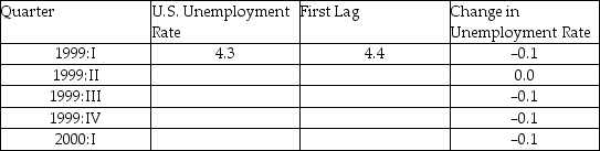 (c)You decide to estimate an AR(1)in the change in the United States unemployment rate to forecast the aggregate unemployment rate. The result is as follows:
  = -0.003 + 0.621 ? UrateUSt-1, R2 = 0.393, SER = 0.255
(0.022)(0.106)
The AR(1)coefficient for the change in the inflation rate was 0.211 and the regression R2 was 0.04. What does the difference in the results suggest here?
(d)The textbook used the change in the log of the price level to approximate the inflation rate, and then predicted the change in the inflation rate. Why aren't logarithms used here?
(e)If much of the forecast error arises as a result of future error terms dominating the error resulting from estimating the unknown coefficients, then what is your best guess of the RMSFE here?
(f)The actual unemployment rate during the fourth quarter of 1999 is 4.1 percent, and it decreased from the third quarter to the fourth quarter by 0.1 percent. What is your forecast for the unemployment rate level in the first quarter of 1996?
(g)You want to see how sensitive your forecast is to changes in the specification. Given that you have estimated the regression with quarterly data, you consider an AR(4)model. This results in the following output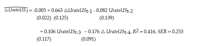
What is your forecast for the unemployment rate level in 2000:I? Compare the forecast error of the AR(4)model with the forecast error of the AR(1)model.
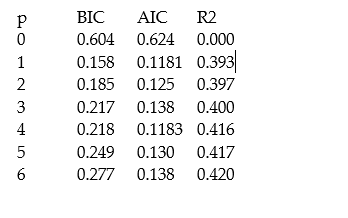
(h)There does not seem to be much difference in the forecast of the unemployment rate level, whether you use the AR(1)or the AR(4). Given the various information criteria and the regression R2 below, which model should you use for forecasting?
(a)The following table presents the first four autocorrelations for the United States aggregate unemployment rate and its change for the time period 1960 (first quarter)to 1999 (fourth quarter). Explain briefly what these two autocorrelations measure.
First Four Autocorrelations of the U.S. Unemployment Rate and Its Change,
1960:I - 1999:IV
(b)The accompanying table gives changes in the United States aggregate unemployment rate for the period 1999:I-2000:I and levels of the current and lagged unemployment rates for 1999:I. Fill in the blanks for the missing unemployment rate levels.Changes in Unemployment Rates in the United States
First Quarter 1999 to First Quarter 2000
(c)You decide to estimate an AR(1)in the change in the United States unemployment rate to forecast the aggregate unemployment rate. The result is as follows: = -0.003 + 0.621 ? UrateUSt-1, R2 = 0.393, SER = 0.255(0.022)(0.106)
The AR(1)coefficient for the change in the inflation rate was 0.211 and the regression R2 was 0.04. What does the difference in the results suggest here?
(d)The textbook used the change in the log of the price level to approximate the inflation rate, and then predicted the change in the inflation rate. Why aren't logarithms used here?
(e)If much of the forecast error arises as a result of future error terms dominating the error resulting from estimating the unknown coefficients, then what is your best guess of the RMSFE here?
(f)The actual unemployment rate during the fourth quarter of 1999 is 4.1 percent, and it decreased from the third quarter to the fourth quarter by 0.1 percent. What is your forecast for the unemployment rate level in the first quarter of 1996?
(g)You want to see how sensitive your forecast is to changes in the specification. Given that you have estimated the regression with quarterly data, you consider an AR(4)model. This results in the following output
What is your forecast for the unemployment rate level in 2000:I? Compare the forecast error of the AR(4)model with the forecast error of the AR(1)model.
(h)There does not seem to be much difference in the forecast of the unemployment rate level, whether you use the AR(1)or the AR(4). Given the various information criteria and the regression R2 below, which model should you use for forecasting?
سؤال
سؤال
سؤال
Having learned in macroeconomics that consumption depends on disposable income, you want to determine whether or not disposable income helps predict future consumption. You collect data for the sample period 1962:I to 1995:IV and plot the two variables.
(a)To determine whether or not past values of personal disposable income growth rates help to predict consumption growth rates, you estimate the following relationship.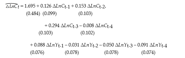
The Granger causality test for the exclusion on all four lags of the GDP growth rate is 0.98. Find the critical value for the 1%, the 5%, and the 10% level from the relevant table and make a decision on whether or not these additional variables Granger cause the change in the growth rate of consumption.
(b)You are somewhat surprised about the result in the previous question and wonder, how sensitive it is with regard to the lag length in the ADL(p,q)model. As a result, you calculate BIC and AIC of p and q from 0 to 6. The results are displayed in the accompanying table: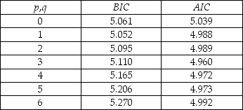 Which values for p and q should you choose?
(c)Estimating an ADL(1,1)model gives you a t-statistic of 1.28 on the coefficient of lagged disposable income growth. What does the Granger causality test suggest about the inclusion of lagged income growth as a predictor of consumption growth?
(a)To determine whether or not past values of personal disposable income growth rates help to predict consumption growth rates, you estimate the following relationship.
The Granger causality test for the exclusion on all four lags of the GDP growth rate is 0.98. Find the critical value for the 1%, the 5%, and the 10% level from the relevant table and make a decision on whether or not these additional variables Granger cause the change in the growth rate of consumption.
(b)You are somewhat surprised about the result in the previous question and wonder, how sensitive it is with regard to the lag length in the ADL(p,q)model. As a result, you calculate BIC and AIC of p and q from 0 to 6. The results are displayed in the accompanying table:
Which values for p and q should you choose?(c)Estimating an ADL(1,1)model gives you a t-statistic of 1.28 on the coefficient of lagged disposable income growth. What does the Granger causality test suggest about the inclusion of lagged income growth as a predictor of consumption growth?
سؤال
سؤال
سؤال
You have collected quarterly data on Canadian unemployment (UrateC)and inflation (InfC)from 1962 to 1999 with the aim to forecast Canadian inflation.
(a)To get a better feel for the data, you first inspect the plots for the series.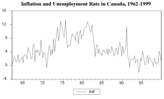
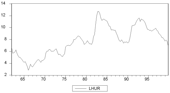 Inspecting the Canadian inflation rate plot and having calculated the first autocorrelation to be 0.79 for the sample period, do you suspect that the Canadian inflation rate has a stochastic trend? What more formal methods do you have available to test for a unit root?
(b)You run the following regression, where the numbers in parenthesis are homoskedasticity-only standard errors: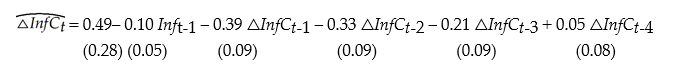
Test for the presence of a stochastic trend. Should you have used heteroskedasticity-robust standard errors? Does the fact that you use quarterly data suggest including four lags in the above regression, or how should you determine the number of lags?
(c)To forecast the Canadian inflation rate for 2000:I, you estimate an AR(1), AR(4), and an ADL(4,1)model for the sample period 1962:I to 1999:IV. The results are as follows: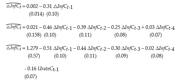
In addition, you have the following information on inflation in Canada during the four quarters of 1999 and the first quarter of 2000:
Inflation and Unemployment in Canada, First Quarter 1999 to First Quarter 2000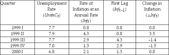 For each of the three models, calculate the predicted inflation rate for the period 2000:I and the forecast error.
(d)Perform a test on whether or not Canadian unemployment rates Granger-cause the Canadian inflation rate.
(a)To get a better feel for the data, you first inspect the plots for the series.
Inspecting the Canadian inflation rate plot and having calculated the first autocorrelation to be 0.79 for the sample period, do you suspect that the Canadian inflation rate has a stochastic trend? What more formal methods do you have available to test for a unit root?(b)You run the following regression, where the numbers in parenthesis are homoskedasticity-only standard errors:
Test for the presence of a stochastic trend. Should you have used heteroskedasticity-robust standard errors? Does the fact that you use quarterly data suggest including four lags in the above regression, or how should you determine the number of lags?
(c)To forecast the Canadian inflation rate for 2000:I, you estimate an AR(1), AR(4), and an ADL(4,1)model for the sample period 1962:I to 1999:IV. The results are as follows:
In addition, you have the following information on inflation in Canada during the four quarters of 1999 and the first quarter of 2000:
Inflation and Unemployment in Canada, First Quarter 1999 to First Quarter 2000
For each of the three models, calculate the predicted inflation rate for the period 2000:I and the forecast error.(d)Perform a test on whether or not Canadian unemployment rates Granger-cause the Canadian inflation rate.
سؤال
سؤال
سؤال
(Requires Appendix material)Define the difference operator Δ = (1 - L)where L is the lag operator, such that LjYt = Yt-j. In general,  = (1- Lj)i, where i and j are typically omitted when they take the value of 1. Show the expressions in Y only when applying the difference operator to the following expressions, and give the resulting expression an economic interpretation, assuming that you are working with quarterly data:
(a)Δ4Yt
(b) Yt
Yt
(c)
 Yt
Yt
(d) Yt
Yt
= (1- Lj)i, where i and j are typically omitted when they take the value of 1. Show the expressions in Y only when applying the difference operator to the following expressions, and give the resulting expression an economic interpretation, assuming that you are working with quarterly data:(a)Δ4Yt
(b)
Yt(c)
Yt(d)
Yt سؤال
سؤال
سؤال
Consider the standard AR(1)Yt = β0 + β1Yt-1 + ut, where the usual assumptions hold.
(a)Show that yt = β0Yt-1 + ut, where yt is Yt with the mean removed, i.e., yt = Yt - E(Yt). Show that E(Yt)= 0.
(b)Show that the r-period ahead forecast E( +r
+r
 )=
)= 
 If 0 < β1 < 1, how does the r-period ahead forecast behave as r becomes large? What is the forecast of
  for large r?
(c)The median lag is the number of periods it takes a time series with zero mean to halve its current value (in expectation), i.e., the solution r to E( +r
+r
 )= 0.5
  Show that in the present case this is given by r = -
(a)Show that yt = β0Yt-1 + ut, where yt is Yt with the mean removed, i.e., yt = Yt - E(Yt). Show that E(Yt)= 0.
(b)Show that the r-period ahead forecast E(
+r )= If 0 < β1 < 1, how does the r-period ahead forecast behave as r becomes large? What is the forecast of for large r?(c)The median lag is the number of periods it takes a time series with zero mean to halve its current value (in expectation), i.e., the solution r to E(
+r )= 0.5 Show that in the present case this is given by r = - سؤال
Consider the AR(1)model Yt = β0 + β1Yt-1 + ut,  < 1..
< 1..
(a)Find the mean and variance of Yt.
(b)Find the first two autocovariances of Yt.
(c)Find the first two autocorrelations of Yt.
< 1..(a)Find the mean and variance of Yt.
(b)Find the first two autocovariances of Yt.
(c)Find the first two autocorrelations of Yt.
سؤال
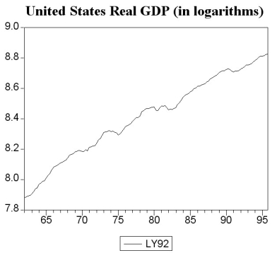
The following two graphs give you a plot of the United States aggregate unemployment rate for the sample period 1962:I to 1999:IV, and the (log)level of real United States GDP for the sample period 1962:I to 1995:IV. You want test for stationarity in both cases. Indicate whether or not you should include a time trend in your Augmented Dickey-Fuller test and why. 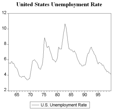
سؤال
You have decided to use the Dickey Fuller (DF)test on the United States aggregate unemployment rate (sample period 1962:I - 1995:IV). As a result, you estimate the following AR(1)model  t = 0.114 - 0.024 UrateUSt-1, R2 = 0.0118, SER = 0.3417
(0.121)(0.019)
You recall that your textbook mentioned that this form of the AR(1)is convenient because it allows for you to test for the presence of a unit root by using the t- statistic of the slope. Being adventurous, you decide to estimate the original form of the AR(1)instead, which results in the following output t = 0.114 - 0.976 UrateUSt-1, R2 = 0.9510, SER = 0.3417
(0.121)(0.019)
You are surprised to find the constant, the standard errors of the two coefficients, and the SER unchanged, while the regression R2 increased substantially. Explain this increase in the regression R2. Why should you have been able to predict the change in the slope coefficient and the constancy of the standard errors of the two coefficients and the SER?
t = 0.114 - 0.024 UrateUSt-1, R2 = 0.0118, SER = 0.3417(0.121)(0.019)
You recall that your textbook mentioned that this form of the AR(1)is convenient because it allows for you to test for the presence of a unit root by using the t- statistic of the slope. Being adventurous, you decide to estimate the original form of the AR(1)instead, which results in the following output
t = 0.114 - 0.976 UrateUSt-1, R2 = 0.9510, SER = 0.3417(0.121)(0.019)
You are surprised to find the constant, the standard errors of the two coefficients, and the SER unchanged, while the regression R2 increased substantially. Explain this increase in the regression R2. Why should you have been able to predict the change in the slope coefficient and the constancy of the standard errors of the two coefficients and the SER?
سؤال
سؤال
(Requires Appendix material)The long-run, stationary state solution of an AD(p,q)model, which can be written as A(L)Yt = ?0 + c(L)Xt-1 + ut, where  = 1, and
  = -?j, cj = ?j, can be found by setting L=1 in the two lag polynomials. Explain. Derive the long-run solution for the estimated ADL(4,4)of the change in the inflation rate on unemployment:
 t = 1.32 - .36 ?Inft-1 - 0.34vInft-2 + 0.7?Inft-3 - 0.3?Inft-4
-2.68Unempt-1 + 3.43Unempt-2 - 1.04Unempt-3 + .07Unempt-4
Assume that the inflation rate is constant in the long-run and calculate the resulting unemployment rate. What does the solution represent? Is it reasonable to assume that this long-run solution is constant over the estimation period 1962-1999? If not, how could you detect the instability?
= 1, and = -?j, cj = ?j, can be found by setting L=1 in the two lag polynomials. Explain. Derive the long-run solution for the estimated ADL(4,4)of the change in the inflation rate on unemployment: t = 1.32 - .36 ?Inft-1 - 0.34vInft-2 + 0.7?Inft-3 - 0.3?Inft-4-2.68Unempt-1 + 3.43Unempt-2 - 1.04Unempt-3 + .07Unempt-4
Assume that the inflation rate is constant in the long-run and calculate the resulting unemployment rate. What does the solution represent? Is it reasonable to assume that this long-run solution is constant over the estimation period 1962-1999? If not, how could you detect the instability?
سؤال
Consider the following model
Yt = α0 + α1
 + ut
+ ut
where the superscript "e" indicates expected values. This may represent an example where consumption depended on expected, or "permanent," income. Furthermore, let expected income be formed as follows: =
=  + λ(Xt-1 -
  ); 0 < λ < 1
This particular type of expectation formation is called the "adaptive expectations hypothesis."
(a)In the above expectation formation hypothesis, expectations are formed at the beginning of the period, say the 1st of January if you had annual data. Give an intuitive explanation for this process.
(b)Transform the adaptive expectation hypothesis in such a way that the right hand side of the equation only contains observable variables, i.e., no expectations.
(c)Show that by substituting the resulting equation from the previous question into the original equation, you get an ADL(0, ∞)type equation. How are the coefficients of the regressors related to each other?
(d)Can you think of a transformation of the ADL(0, ∞)equation into an ADL(1,1)type equation, if you allowed the error term to be (ut - λut-1)?
Yt = α0 + α1
+ utwhere the superscript "e" indicates expected values. This may represent an example where consumption depended on expected, or "permanent," income. Furthermore, let expected income be formed as follows:
= + λ(Xt-1 - ); 0 < λ < 1This particular type of expectation formation is called the "adaptive expectations hypothesis."
(a)In the above expectation formation hypothesis, expectations are formed at the beginning of the period, say the 1st of January if you had annual data. Give an intuitive explanation for this process.
(b)Transform the adaptive expectation hypothesis in such a way that the right hand side of the equation only contains observable variables, i.e., no expectations.
(c)Show that by substituting the resulting equation from the previous question into the original equation, you get an ADL(0, ∞)type equation. How are the coefficients of the regressors related to each other?
(d)Can you think of a transformation of the ADL(0, ∞)equation into an ADL(1,1)type equation, if you allowed the error term to be (ut - λut-1)?
سؤال
You have collected data for real GDP (Y)and have estimated the following function:
ln t = 7.866 + 0.00679×Zeit
(0.007)(0.00008)
t = 1961:I - 2007:IV, R2 = 0.98, SER = 0.036
where Zeit is a deterministic time trend, which takes on the value of 1 during the first quarter of 1961, and is increased by one for each following quarter.
a. Interpret the slope coefficient. Does it make sense?
b. Interpret the regression R2. Are you impressed by its value?
c. Do you think that given the regression R2, you should use the equation to forecast real GDP beyond the sample period?
ln
t = 7.866 + 0.00679×Zeit(0.007)(0.00008)
t = 1961:I - 2007:IV, R2 = 0.98, SER = 0.036
where Zeit is a deterministic time trend, which takes on the value of 1 during the first quarter of 1961, and is increased by one for each following quarter.
a. Interpret the slope coefficient. Does it make sense?
b. Interpret the regression R2. Are you impressed by its value?
c. Do you think that given the regression R2, you should use the equation to forecast real GDP beyond the sample period?
سؤال
(Requires Appendix material): Show that the AR(1)process Yt = a1Yt-1 + et;  < 1, can be converted to a MA(∞)process.
< 1, can be converted to a MA(∞)process.
فتح الحزمة
قم بالتسجيل لفتح البطاقات في هذه المجموعة!
Unlock Deck
Unlock Deck
1/50
العب
ملء الشاشة (f)
Deck 14: Introduction to Time Series Regression and Forecasting
1
To choose the number of lags in either an autoregression or in a time series regression model with multiple predictors, you can use any of the following test statistics with the exception of the
A)F-statistic.
B)Akaike Information Criterion.
C)Bayes Information Criterion.
D)Augmented Dickey-Fuller test.
A)F-statistic.
B)Akaike Information Criterion.
C)Bayes Information Criterion.
D)Augmented Dickey-Fuller test.
D
2
An autoregression is a regression
A)of a dependent variable on lags of regressors.
B)that allows for the errors to be correlated.
C)model that relates a time series variable to its past values.
D)to predict sales in a certain industry.
A)of a dependent variable on lags of regressors.
B)that allows for the errors to be correlated.
C)model that relates a time series variable to its past values.
D)to predict sales in a certain industry.
C
3
Autoregressive distributed lag models include
A)current and lagged values of the error term.
B)lags of the dependent variable, and lagged values of additional predictor variables.
C)current and lagged values of the residuals.
D)lags and leads of the dependent variable.
A)current and lagged values of the error term.
B)lags of the dependent variable, and lagged values of additional predictor variables.
C)current and lagged values of the residuals.
D)lags and leads of the dependent variable.
B
4
Pseudo out of sample forecasting can be used for the following reasons with the exception of
A)giving the forecaster a sense of how well the model forecasts at the end of the sample.
B)estimating the RMSFE.
C)analyzing whether or not a time series contains a unit root.
D)evaluating the relative forecasting performance of two or more forecasting models.
A)giving the forecaster a sense of how well the model forecasts at the end of the sample.
B)estimating the RMSFE.
C)analyzing whether or not a time series contains a unit root.
D)evaluating the relative forecasting performance of two or more forecasting models.
فتح الحزمة
افتح القفل للوصول البطاقات البالغ عددها 50 في هذه المجموعة.
فتح الحزمة
k this deck
5
Time series variables fail to be stationary when
A)the economy experiences severe fluctuations.
B)the population regression has breaks.
C)there is strong seasonal variation in the data.
D)there are no trends.
A)the economy experiences severe fluctuations.
B)the population regression has breaks.
C)there is strong seasonal variation in the data.
D)there are no trends.
فتح الحزمة
افتح القفل للوصول البطاقات البالغ عددها 50 في هذه المجموعة.
فتح الحزمة
k this deck
6
The root mean squared forecast error (RMSFE)is defined as
A)
B)
C)
D)
A)
B)
C)
D)
فتح الحزمة
افتح القفل للوصول البطاقات البالغ عددها 50 في هذه المجموعة.
فتح الحزمة
k this deck
7
Stationarity means that the
A)error terms are not correlated.
B)probability distribution of the time series variable does not change over time.
C)time series has a unit root.
D)forecasts remain within 1.96 standard deviation outside the sample period.
A)error terms are not correlated.
B)probability distribution of the time series variable does not change over time.
C)time series has a unit root.
D)forecasts remain within 1.96 standard deviation outside the sample period.
فتح الحزمة
افتح القفل للوصول البطاقات البالغ عددها 50 في هذه المجموعة.
فتح الحزمة
k this deck
8
The time interval between observations can be all of the following with the exception of data collected
A)daily.
B)by decade.
C)bi-weekly.
D)across firms.
A)daily.
B)by decade.
C)bi-weekly.
D)across firms.
فتح الحزمة
افتح القفل للوصول البطاقات البالغ عددها 50 في هذه المجموعة.
فتح الحزمة
k this deck
9
In order to make reliable forecasts with time series data, all of the following conditions are needed with the exception of
A)coefficients having been estimated precisely.
B)the regression having high explanatory power.
C)the regression being stable.
D)the presence of omitted variable bias.
A)coefficients having been estimated precisely.
B)the regression having high explanatory power.
C)the regression being stable.
D)the presence of omitted variable bias.
فتح الحزمة
افتح القفل للوصول البطاقات البالغ عددها 50 في هذه المجموعة.
فتح الحزمة
k this deck
10
The first difference of the logarithm of Yt equals
A)the first difference of Y.
B)the difference between the lead and the lag of Y.
C)approximately the growth rate of Y when the growth rate is small.
D)the growth rate of Y exactly.
A)the first difference of Y.
B)the difference between the lead and the lag of Y.
C)approximately the growth rate of Y when the growth rate is small.
D)the growth rate of Y exactly.
فتح الحزمة
افتح القفل للوصول البطاقات البالغ عددها 50 في هذه المجموعة.
فتح الحزمة
k this deck
11
The forecast is
A)made for some date beyond the data set used to estimate the regression.
B)another word for the OLS predicted value.
C)equal to the residual plus the OLS predicted value.
D)close to 1.96 times the standard deviation of Y during the sample.
A)made for some date beyond the data set used to estimate the regression.
B)another word for the OLS predicted value.
C)equal to the residual plus the OLS predicted value.
D)close to 1.96 times the standard deviation of Y during the sample.
فتح الحزمة
افتح القفل للوصول البطاقات البالغ عددها 50 في هذه المجموعة.
فتح الحزمة
k this deck
12
Negative autocorrelation in the change of a variable implies that
A)the variable contains only negative values.
B)the series is not stable.
C)an increase in the variable in one period is, on average, associated with a decrease in the next.
D)the data is negatively trended.
A)the variable contains only negative values.
B)the series is not stable.
C)an increase in the variable in one period is, on average, associated with a decrease in the next.
D)the data is negatively trended.
فتح الحزمة
افتح القفل للوصول البطاقات البالغ عددها 50 في هذه المجموعة.
فتح الحزمة
k this deck
13
The Granger Causality Test
A)uses the F-statistic to test the hypothesis that certain regressors have no predictive content for the dependent variable beyond that contained in the other regressors.
B)establishes the direction of causality (as used in common parlance)between X and Y in addition to correlation.
C)is a rather complicated test for statistical independence.
D)is a special case of the Augmented Dickey-Fuller test.
فتح الحزمة
افتح القفل للوصول البطاقات البالغ عددها 50 في هذه المجموعة.
فتح الحزمة
k this deck
14
The Times Series Regression with Multiple Predictors
A)is the same as the ADL(p,q)with additional predictors and their lags present.
B)gives you more than one prediction.
C)cannot be estimated by OLS due to the presence of multiple lags.
D)requires that the k regressors and the dependent variable have nonzero, finite eighth moments.
A)is the same as the ADL(p,q)with additional predictors and their lags present.
B)gives you more than one prediction.
C)cannot be estimated by OLS due to the presence of multiple lags.
D)requires that the k regressors and the dependent variable have nonzero, finite eighth moments.
فتح الحزمة
افتح القفل للوصول البطاقات البالغ عددها 50 في هذه المجموعة.
فتح الحزمة
k this deck
15
One reason for computing the logarithms (ln), or changes in logarithms, of economic time series is that
A)numbers often get very large.
B)economic variables are hardly ever negative.
C)they often exhibit growth that is approximately exponential.
D)natural logarithms are easier to work with than base 10 logarithms.
A)numbers often get very large.
B)economic variables are hardly ever negative.
C)they often exhibit growth that is approximately exponential.
D)natural logarithms are easier to work with than base 10 logarithms.
فتح الحزمة
افتح القفل للوصول البطاقات البالغ عددها 50 في هذه المجموعة.
فتح الحزمة
k this deck
16
One of the sources of error in the RMSFE in the AR(1)model is
A)the error in estimating the coefficients β0 and β1.
B)due to measuring variables in logarithms.
C)that the value of the explanatory variable is not known with certainty when making a forecast.
D)the model only looks at the previous period's value of Y when the entire history should be taken into account.
فتح الحزمة
افتح القفل للوصول البطاقات البالغ عددها 50 في هذه المجموعة.
فتح الحزمة
k this deck
17
The jth autocorrelation coefficient is defined as
A)
B)
C)
D)
A)
B)
C)
D)
فتح الحزمة
افتح القفل للوصول البطاقات البالغ عددها 50 في هذه المجموعة.
فتح الحزمة
k this deck
18
The ADL(p,q)model is represented by the following equation
A)Yt = β0 + βpYt-p + δqXt-q + ut.
B)Yt = β0 + β1Yt-1 + β2Yt-2 + ... + βpYt-p + δqut-q.
C)Yt = β0 + β1Yt-1 + β2Yt-2 + ... + βpYt-p + δ0 + δ1Xt-1 + ut-q.
D)Yt = β0 + β1Yt-1 + β2Yt-2 + ... + βpYt-p + δ1Xt-1 + δ2Xt-2 + ... + δqXt-q + ut.
A)Yt = β0 + βpYt-p + δqXt-q + ut.
B)Yt = β0 + β1Yt-1 + β2Yt-2 + ... + βpYt-p + δqut-q.
C)Yt = β0 + β1Yt-1 + β2Yt-2 + ... + βpYt-p + δ0 + δ1Xt-1 + ut-q.
D)Yt = β0 + β1Yt-1 + β2Yt-2 + ... + βpYt-p + δ1Xt-1 + δ2Xt-2 + ... + δqXt-q + ut.
فتح الحزمة
افتح القفل للوصول البطاقات البالغ عددها 50 في هذه المجموعة.
فتح الحزمة
k this deck
19
The AR(p)model
A)is defined as Yt = β0 + βpYt-p + ut.
B)represents Yt as a linear function of p of its lagged values.
C)can be represented as follows: Yt = β0 + β1Xt + βpYt-p + ut.
D)can be written as Yt = β0 + β1Yt-1 + ut-p.
A)is defined as Yt = β0 + βpYt-p + ut.
B)represents Yt as a linear function of p of its lagged values.
C)can be represented as follows: Yt = β0 + β1Xt + βpYt-p + ut.
D)can be written as Yt = β0 + β1Yt-1 + ut-p.
فتح الحزمة
افتح القفل للوصول البطاقات البالغ عددها 50 في هذه المجموعة.
فتح الحزمة
k this deck
20
Departures from stationarity
A)jeopardize forecasts and inference based on time series regression.
B)occur often in cross-sectional data.
C)can be made to have less severe consequences by using log-log specifications.
D)cannot be fixed.
A)jeopardize forecasts and inference based on time series regression.
B)occur often in cross-sectional data.
C)can be made to have less severe consequences by using log-log specifications.
D)cannot be fixed.
فتح الحزمة
افتح القفل للوصول البطاقات البالغ عددها 50 في هذه المجموعة.
فتح الحزمة
k this deck
21
You should use the QLR test for breaks in the regression coefficients, when
A)the Chow F-test has a p value of between 0.05 and 0.10.
B)the suspected break data is not known.
C)there are breaks in only some, but not all, of the regression coefficients.
D)the suspected break data is known.
A)the Chow F-test has a p value of between 0.05 and 0.10.
B)the suspected break data is not known.
C)there are breaks in only some, but not all, of the regression coefficients.
D)the suspected break data is known.
فتح الحزمة
افتح القفل للوصول البطاقات البالغ عددها 50 في هذه المجموعة.
فتح الحزمة
k this deck
22
The Akaike Information Criterion (AIC)is given by the following formula
A)AIC(p)= ln [ ] + (p+1)
B)AIC(p)= ln [ ] + (p+1)
C)AIC(p)= ln [ ] +
D)AIC(p)= ln [ ] × (p+1)
A)AIC(p)= ln [ ] + (p+1)
B)AIC(p)= ln [ ] + (p+1)
C)AIC(p)= ln [ ] +
D)AIC(p)= ln [ ] × (p+1)
فتح الحزمة
افتح القفل للوصول البطاقات البالغ عددها 50 في هذه المجموعة.
فتح الحزمة
k this deck
23
If a "break" occurs in the population regression function, then
A)inference and forecasting are compromised when neglecting it.
B)an Augmented Dickey Fuller test, rather than the Dickey Fuller test, should be used to test for stationarity.
C)this suggests the presence of a deterministic trend in addition to a stochastic trend.
D)forecasting, but not inference, is unaffected, if the break occurs during the first half of the sample period.
فتح الحزمة
افتح القفل للوصول البطاقات البالغ عددها 50 في هذه المجموعة.
فتح الحزمة
k this deck
24
The textbook displayed the accompanying four economic time series with "markedly different patterns." For each indicate what you think the sample autocorrelations of the level (Y)and change (△Y)will be and explain your reasoning.
(a) (b) (c) (d)
(a)
(b) (c) (d) فتح الحزمة
افتح القفل للوصول البطاقات البالغ عددها 50 في هذه المجموعة.
فتح الحزمة
k this deck
25
Problems caused by stochastic trends include all of the following with the exception of
A)the estimator of an AR(1)is biased towards zero if it's true value is one.
B)the model can no longer be estimated by OLS.
C)t-statistics on regression coefficients can have a nonnormal distribution, even in large samples.
D)the presence of spurious regression..
A)the estimator of an AR(1)is biased towards zero if it's true value is one.
B)the model can no longer be estimated by OLS.
C)t-statistics on regression coefficients can have a nonnormal distribution, even in large samples.
D)the presence of spurious regression..
فتح الحزمة
افتح القفل للوصول البطاقات البالغ عددها 50 في هذه المجموعة.
فتح الحزمة
k this deck
26
There is some evidence that the Phillips curve has been unstable during the 1962 to 1999 period for the United States, and in particular during the 1990s. You set out to investigate whether or not this instability also occurred in other places. Canada is a particularly interesting case, due to its proximity to the United States and the fact that many features of its economy are similar to that of the U.S.
(a)Reading up on some of the comparative economic performance literature, you find that Canadian unemployment rates were roughly the same as U.S. unemployment rates from the 1920s to the early 1980s. The accompanying figure shows that a gap opened between the unemployment rates of the two countries in 1982, which has persisted to this date. Inspection of the graph and data suggest that the break occurred during the second quarter of 1982. To investigate whether the Canadian Phillips curve shows a break at that point, you estimate an ADL(4,4)model for the sample period 1962:I-1999:IV and perform a Chow test. Specifically you postulate that the constant and coefficients of the unemployment rates changed at that point. The F-statistic is 1.96. Find the critical value from the F-table and test the null hypothesis that a break occurred at that time. Is there any reason why you should be skeptical about the result regarding the break and using the Chow-test to detect it?
(b)You consider alternative ways to test for a break in the relationship. The accompanying figure shows the F-statistics testing for a break in the ADL(4,4)equation at different dates. The QLR-statistic with 15% trimming is 3.11. Comment on the figure and test for the hypothesis of a break in the ADL(4,4)regression.
(c)To test for the stability of the Canadian Phillips curve in the 1990s, you decide to perform a pseudo out-of-sample forecasting. For the 24 quarters from 1994:I-1999:IV you use the ADL(4,4)model to calculate the forecasted change in the inflation rate, the resulting forecasted inflation rate, and the forecast error. The standard error of the ADL(4,4)for the estimation sample period 1962:1-1993:4 is 1.91 and the sample RMSFE is 1.70. The average forecast error for the 24 inflation rates is 0.003 and the sample standard deviation of the forecast errors is 0.82. Calculate the t-statistic and test the hypothesis that the mean out-of-sample forecast error is zero. Comment on the result and the accompanying figure of the actual and forecasted inflation rate.
(a)Reading up on some of the comparative economic performance literature, you find that Canadian unemployment rates were roughly the same as U.S. unemployment rates from the 1920s to the early 1980s. The accompanying figure shows that a gap opened between the unemployment rates of the two countries in 1982, which has persisted to this date.
Inspection of the graph and data suggest that the break occurred during the second quarter of 1982. To investigate whether the Canadian Phillips curve shows a break at that point, you estimate an ADL(4,4)model for the sample period 1962:I-1999:IV and perform a Chow test. Specifically you postulate that the constant and coefficients of the unemployment rates changed at that point. The F-statistic is 1.96. Find the critical value from the F-table and test the null hypothesis that a break occurred at that time. Is there any reason why you should be skeptical about the result regarding the break and using the Chow-test to detect it?(b)You consider alternative ways to test for a break in the relationship. The accompanying figure shows the F-statistics testing for a break in the ADL(4,4)equation at different dates.
The QLR-statistic with 15% trimming is 3.11. Comment on the figure and test for the hypothesis of a break in the ADL(4,4)regression.(c)To test for the stability of the Canadian Phillips curve in the 1990s, you decide to perform a pseudo out-of-sample forecasting. For the 24 quarters from 1994:I-1999:IV you use the ADL(4,4)model to calculate the forecasted change in the inflation rate, the resulting forecasted inflation rate, and the forecast error. The standard error of the ADL(4,4)for the estimation sample period 1962:1-1993:4 is 1.91 and the sample RMSFE is 1.70. The average forecast error for the 24 inflation rates is 0.003 and the sample standard deviation of the forecast errors is 0.82. Calculate the t-statistic and test the hypothesis that the mean out-of-sample forecast error is zero. Comment on the result and the accompanying figure of the actual and forecasted inflation rate.
فتح الحزمة
افتح القفل للوصول البطاقات البالغ عددها 50 في هذه المجموعة.
فتح الحزمة
k this deck
27
The random walk model is an example of a
A)deterministic trend model.
B)binomial model.
C)stochastic trend model.
D)stationary model.
A)deterministic trend model.
B)binomial model.
C)stochastic trend model.
D)stationary model.
فتح الحزمة
افتح القفل للوصول البطاقات البالغ عددها 50 في هذه المجموعة.
فتح الحزمة
k this deck
28
You collect monthly data on the money supply (M2)for the United States from 1962:1-2002:4 to forecast future money supply behavior. where LM2 and DLM2 are the log level and growth rate of M2.
(a)Using quarterly data, when analyzing inflation and unemployment in the United States, the textbook converted log levels of variables into growth rates by differencing the log levels, and then multiplying these by 400. Given that you have monthly data, how would you proceed here?
(b)How would you go about testing for a stochastic trend in LM2 and DLM2? Be specific about how to decide the number of lags to be included and whether or not to include a deterministic trend in your test. The textbook found the (quarterly)inflation rate to have a unit root. Does this have any affect on your expectation about whether or not the (monthly)money growth rate should be stationary?
(c)You decide to conduct an ADF unit root test for LM2, DLM2, and the change in the growth rate ΔDLM2. This results in the following t-statistic on the parameter of interest. Find the critical value at the 1%, 5%, and 10% level and decide which of the coefficients is significant. What is the alternative hypothesis?
(d)In forecasting the money growth rate, you add lags of the monetary base growth rate (DLMB)to see if you can improve on the forecasting performance of a chosen AR(10)model in DLM2. You perform a Granger causality test on the 9 lags of DLMB and find a F-statistic of 2.31. Discuss the implications.
(e)Curious about the result in the previous question, you decide to estimate an ADL(10,10)for DLMB and calculate the F-statistic for the Granger causality test on the 9 lag coefficients of DLM2. This turns out to be 0.66. Discuss.
(f)Is there any a priori reason for you to be skeptical of the results? What other tests should you perform?
where LM2 and DLM2 are the log level and growth rate of M2.(a)Using quarterly data, when analyzing inflation and unemployment in the United States, the textbook converted log levels of variables into growth rates by differencing the log levels, and then multiplying these by 400. Given that you have monthly data, how would you proceed here?
(b)How would you go about testing for a stochastic trend in LM2 and DLM2? Be specific about how to decide the number of lags to be included and whether or not to include a deterministic trend in your test. The textbook found the (quarterly)inflation rate to have a unit root. Does this have any affect on your expectation about whether or not the (monthly)money growth rate should be stationary?
(c)You decide to conduct an ADF unit root test for LM2, DLM2, and the change in the growth rate ΔDLM2. This results in the following t-statistic on the parameter of interest.
Find the critical value at the 1%, 5%, and 10% level and decide which of the coefficients is significant. What is the alternative hypothesis?(d)In forecasting the money growth rate, you add lags of the monetary base growth rate (DLMB)to see if you can improve on the forecasting performance of a chosen AR(10)model in DLM2. You perform a Granger causality test on the 9 lags of DLMB and find a F-statistic of 2.31. Discuss the implications.
(e)Curious about the result in the previous question, you decide to estimate an ADL(10,10)for DLMB and calculate the F-statistic for the Granger causality test on the 9 lag coefficients of DLM2. This turns out to be 0.66. Discuss.
(f)Is there any a priori reason for you to be skeptical of the results? What other tests should you perform?
فتح الحزمة
افتح القفل للوصول البطاقات البالغ عددها 50 في هذه المجموعة.
فتح الحزمة
k this deck
29
(Requires Internet access for the test question)
The following question requires you to download data from the internet and to load it into a statistical package such as STATA or EViews.
a. Your textbook suggests using two test statistics to test for stationarity: DF and ADF. Test the null hypothesis that inflation has a stochastic trend against the alternative that it is stationary by performing the DF and ADF test for a unit autoregressive root. That is, use the equation (14.34)in your textbook with four lags and without a lag of the change in the inflation rate as a regressor for sample period 1962:I - 2004:IV. Go to the Stock and Watson companion website for the textbook and download the data "Macroeconomic Data Used in Chapters 14 and 16." Enter the data for consumer price index, calculate the inflation rate and the acceleration of the inflation rate, and replicate the result on page 526 of your textbook. Make sure not to use the heteroskedasticity-robust standard error option for the estimation.
b. Next find a website with more recent data, such as the Federal Reserve Economic Data (FRED)site at the Federal Reserve Bank of St. Louis. Locate the data for the CPI, which will be monthly, and convert the data in quarterly averages. Then, using a sample from 1962:I - 2009:IV, re-estimate the above specification and comment on the changes that have occurred.
c. For the new sample period, find the DF statistic.
d. Finally, calculate the ADF statistic, allowing for the lag length of the inflation acceleration term to be determined by either the AIC or the BIC.
فتح الحزمة
افتح القفل للوصول البطاقات البالغ عددها 50 في هذه المجموعة.
فتح الحزمة
k this deck
30
You set out to forecast the unemployment rate in the United States (UrateUS), using quarterly data from 1960, first quarter, to 1999, fourth quarter.
(a)The following table presents the first four autocorrelations for the United States aggregate unemployment rate and its change for the time period 1960 (first quarter)to 1999 (fourth quarter). Explain briefly what these two autocorrelations measure.
First Four Autocorrelations of the U.S. Unemployment Rate and Its Change,
1960:I - 1999:IV (b)The accompanying table gives changes in the United States aggregate unemployment rate for the period 1999:I-2000:I and levels of the current and lagged unemployment rates for 1999:I. Fill in the blanks for the missing unemployment rate levels.
Changes in Unemployment Rates in the United States
First Quarter 1999 to First Quarter 2000 (c)You decide to estimate an AR(1)in the change in the United States unemployment rate to forecast the aggregate unemployment rate. The result is as follows: = -0.003 + 0.621 ? UrateUSt-1, R2 = 0.393, SER = 0.255
(0.022)(0.106)
The AR(1)coefficient for the change in the inflation rate was 0.211 and the regression R2 was 0.04. What does the difference in the results suggest here?
(d)The textbook used the change in the log of the price level to approximate the inflation rate, and then predicted the change in the inflation rate. Why aren't logarithms used here?
(e)If much of the forecast error arises as a result of future error terms dominating the error resulting from estimating the unknown coefficients, then what is your best guess of the RMSFE here?
(f)The actual unemployment rate during the fourth quarter of 1999 is 4.1 percent, and it decreased from the third quarter to the fourth quarter by 0.1 percent. What is your forecast for the unemployment rate level in the first quarter of 1996?
(g)You want to see how sensitive your forecast is to changes in the specification. Given that you have estimated the regression with quarterly data, you consider an AR(4)model. This results in the following output
What is your forecast for the unemployment rate level in 2000:I? Compare the forecast error of the AR(4)model with the forecast error of the AR(1)model.
(h)There does not seem to be much difference in the forecast of the unemployment rate level, whether you use the AR(1)or the AR(4). Given the various information criteria and the regression R2 below, which model should you use for forecasting?
(a)The following table presents the first four autocorrelations for the United States aggregate unemployment rate and its change for the time period 1960 (first quarter)to 1999 (fourth quarter). Explain briefly what these two autocorrelations measure.
First Four Autocorrelations of the U.S. Unemployment Rate and Its Change,
1960:I - 1999:IV
(b)The accompanying table gives changes in the United States aggregate unemployment rate for the period 1999:I-2000:I and levels of the current and lagged unemployment rates for 1999:I. Fill in the blanks for the missing unemployment rate levels.Changes in Unemployment Rates in the United States
First Quarter 1999 to First Quarter 2000
(c)You decide to estimate an AR(1)in the change in the United States unemployment rate to forecast the aggregate unemployment rate. The result is as follows: = -0.003 + 0.621 ? UrateUSt-1, R2 = 0.393, SER = 0.255(0.022)(0.106)
The AR(1)coefficient for the change in the inflation rate was 0.211 and the regression R2 was 0.04. What does the difference in the results suggest here?
(d)The textbook used the change in the log of the price level to approximate the inflation rate, and then predicted the change in the inflation rate. Why aren't logarithms used here?
(e)If much of the forecast error arises as a result of future error terms dominating the error resulting from estimating the unknown coefficients, then what is your best guess of the RMSFE here?
(f)The actual unemployment rate during the fourth quarter of 1999 is 4.1 percent, and it decreased from the third quarter to the fourth quarter by 0.1 percent. What is your forecast for the unemployment rate level in the first quarter of 1996?
(g)You want to see how sensitive your forecast is to changes in the specification. Given that you have estimated the regression with quarterly data, you consider an AR(4)model. This results in the following output
What is your forecast for the unemployment rate level in 2000:I? Compare the forecast error of the AR(4)model with the forecast error of the AR(1)model.
(h)There does not seem to be much difference in the forecast of the unemployment rate level, whether you use the AR(1)or the AR(4). Given the various information criteria and the regression R2 below, which model should you use for forecasting?
فتح الحزمة
افتح القفل للوصول البطاقات البالغ عددها 50 في هذه المجموعة.
فتح الحزمة
k this deck
31
(Requires Internet Access for the test question)
The following question requires you to download data from the internet and to load it into a statistical package such as STATA or EViews.
a. Your textbook estimates an AR(1)model (equation 14.7)for the change in the inflation rate using a sample period 1962:I - 2004:IV. Go to the Stock and Watson companion website for the textbook and download the data "Macroeconomic Data Used in Chapters 14 and 16." Enter the data for consumer price index, calculate the inflation rate, the acceleration of the inflation rate, and replicate the result on page 526 of your textbook. Make sure to use heteroskedasticity-robust standard error option for the estimation.
b. Next find a website with more recent data, such as the Federal Reserve Economic Data (FRED)site at the Federal Reserve Bank of St. Louis. Locate the data for the CPI, which will be monthly, and convert the data in quarterly averages. Then, using a sample from 1962:I - 2009:IV, re-estimate the above specification and comment on the changes that have occurred.
c. Based on the BIC, how many lags should be included in the forecasting equation for the change in the inflation rate? Use the new data set and sample period to answer the question.
فتح الحزمة
افتح القفل للوصول البطاقات البالغ عددها 50 في هذه المجموعة.
فتح الحزمة
k this deck
32
The BIC is a statistic
A)commonly used to test for serial correlation
B)only used in cross-sectional analysis
C)developed by the Bank of England in its river of blood analysis
D)used to help the researcher choose the number of lags in an autoregression
A)commonly used to test for serial correlation
B)only used in cross-sectional analysis
C)developed by the Bank of England in its river of blood analysis
D)used to help the researcher choose the number of lags in an autoregression
فتح الحزمة
افتح القفل للوصول البطاقات البالغ عددها 50 في هذه المجموعة.
فتح الحزمة
k this deck
33
Having learned in macroeconomics that consumption depends on disposable income, you want to determine whether or not disposable income helps predict future consumption. You collect data for the sample period 1962:I to 1995:IV and plot the two variables.
(a)To determine whether or not past values of personal disposable income growth rates help to predict consumption growth rates, you estimate the following relationship.
The Granger causality test for the exclusion on all four lags of the GDP growth rate is 0.98. Find the critical value for the 1%, the 5%, and the 10% level from the relevant table and make a decision on whether or not these additional variables Granger cause the change in the growth rate of consumption.
(b)You are somewhat surprised about the result in the previous question and wonder, how sensitive it is with regard to the lag length in the ADL(p,q)model. As a result, you calculate BIC and AIC of p and q from 0 to 6. The results are displayed in the accompanying table: Which values for p and q should you choose?
(c)Estimating an ADL(1,1)model gives you a t-statistic of 1.28 on the coefficient of lagged disposable income growth. What does the Granger causality test suggest about the inclusion of lagged income growth as a predictor of consumption growth?
(a)To determine whether or not past values of personal disposable income growth rates help to predict consumption growth rates, you estimate the following relationship.
The Granger causality test for the exclusion on all four lags of the GDP growth rate is 0.98. Find the critical value for the 1%, the 5%, and the 10% level from the relevant table and make a decision on whether or not these additional variables Granger cause the change in the growth rate of consumption.
(b)You are somewhat surprised about the result in the previous question and wonder, how sensitive it is with regard to the lag length in the ADL(p,q)model. As a result, you calculate BIC and AIC of p and q from 0 to 6. The results are displayed in the accompanying table:
Which values for p and q should you choose?(c)Estimating an ADL(1,1)model gives you a t-statistic of 1.28 on the coefficient of lagged disposable income growth. What does the Granger causality test suggest about the inclusion of lagged income growth as a predictor of consumption growth?
فتح الحزمة
افتح القفل للوصول البطاقات البالغ عددها 50 في هذه المجموعة.
فتح الحزمة
k this deck
34
The Augmented Dickey Fuller (ADF)t-statistic
A)has a normal distribution in large samples.
B)has the identical distribution whether or not a trend is included or not.
C)is a two-sided test.
D)is an extension of the Dickey-Fuller test when the underlying model is AR(p)rather than AR(1).
A)has a normal distribution in large samples.
B)has the identical distribution whether or not a trend is included or not.
C)is a two-sided test.
D)is an extension of the Dickey-Fuller test when the underlying model is AR(p)rather than AR(1).
فتح الحزمة
افتح القفل للوصول البطاقات البالغ عددها 50 في هذه المجموعة.
فتح الحزمة
k this deck
35
The AIC is a statistic
A)that is used as an alternative to the BIC when the sample size is small (T < 50)
B)often used to test for heteroskedasticity
C)used to help a researcher chose the number of lags in a time series with multiple predictors
D)all of the above
A)that is used as an alternative to the BIC when the sample size is small (T < 50)
B)often used to test for heteroskedasticity
C)used to help a researcher chose the number of lags in a time series with multiple predictors
D)all of the above
فتح الحزمة
افتح القفل للوصول البطاقات البالغ عددها 50 في هذه المجموعة.
فتح الحزمة
k this deck
36
You have collected quarterly data on Canadian unemployment (UrateC)and inflation (InfC)from 1962 to 1999 with the aim to forecast Canadian inflation.
(a)To get a better feel for the data, you first inspect the plots for the series. Inspecting the Canadian inflation rate plot and having calculated the first autocorrelation to be 0.79 for the sample period, do you suspect that the Canadian inflation rate has a stochastic trend? What more formal methods do you have available to test for a unit root?
(b)You run the following regression, where the numbers in parenthesis are homoskedasticity-only standard errors:
Test for the presence of a stochastic trend. Should you have used heteroskedasticity-robust standard errors? Does the fact that you use quarterly data suggest including four lags in the above regression, or how should you determine the number of lags?
(c)To forecast the Canadian inflation rate for 2000:I, you estimate an AR(1), AR(4), and an ADL(4,1)model for the sample period 1962:I to 1999:IV. The results are as follows:
In addition, you have the following information on inflation in Canada during the four quarters of 1999 and the first quarter of 2000:
Inflation and Unemployment in Canada, First Quarter 1999 to First Quarter 2000 For each of the three models, calculate the predicted inflation rate for the period 2000:I and the forecast error.
(d)Perform a test on whether or not Canadian unemployment rates Granger-cause the Canadian inflation rate.
(a)To get a better feel for the data, you first inspect the plots for the series.
Inspecting the Canadian inflation rate plot and having calculated the first autocorrelation to be 0.79 for the sample period, do you suspect that the Canadian inflation rate has a stochastic trend? What more formal methods do you have available to test for a unit root?(b)You run the following regression, where the numbers in parenthesis are homoskedasticity-only standard errors:
Test for the presence of a stochastic trend. Should you have used heteroskedasticity-robust standard errors? Does the fact that you use quarterly data suggest including four lags in the above regression, or how should you determine the number of lags?
(c)To forecast the Canadian inflation rate for 2000:I, you estimate an AR(1), AR(4), and an ADL(4,1)model for the sample period 1962:I to 1999:IV. The results are as follows:
In addition, you have the following information on inflation in Canada during the four quarters of 1999 and the first quarter of 2000:
Inflation and Unemployment in Canada, First Quarter 1999 to First Quarter 2000
For each of the three models, calculate the predicted inflation rate for the period 2000:I and the forecast error.(d)Perform a test on whether or not Canadian unemployment rates Granger-cause the Canadian inflation rate.
فتح الحزمة
افتح القفل للوصول البطاقات البالغ عددها 50 في هذه المجموعة.
فتح الحزمة
k this deck
37
The formulae for the AIC and the BIC are different. The
A)AIC is preferred because it is easier to calculate
B)BIC is preferred because it is a consistent estimator of the lag length
C)difference is irrelevant in practice since both information criteria lead to the same conclusion
D)AIC will typically underestimate p with non-zero probability
A)AIC is preferred because it is easier to calculate
B)BIC is preferred because it is a consistent estimator of the lag length
C)difference is irrelevant in practice since both information criteria lead to the same conclusion
D)AIC will typically underestimate p with non-zero probability
فتح الحزمة
افتح القفل للوصول البطاقات البالغ عددها 50 في هذه المجموعة.
فتح الحزمة
k this deck
38
Statistical inference was a concept that was not too difficult to understand when using cross-sectional data. For example, it is obvious that a population mean is not the same as a sample mean (take weight of students at your college/university as an example). With a bit of thought, it also became clear that the sample mean had a distribution. This meant that there was uncertainty regarding the population mean given the sample information, and that you had to consider confidence intervals when making statements about the population mean. The same concept carried over into the two-dimensional analysis of a simple regression: knowing the height-weight relationship for a sample of students, for example, allowed you to make statements about the population height-weight relationship. In other words, it was easy to understand the relationship between a sample and a population in cross-sections. But what about time-series? Why should you be allowed to make statistical inference about some population, given a sample at hand (using quarterly data from 1962-2010, for example)? Write an essay explaining the relationship between a sample and a population when using time series.
فتح الحزمة
افتح القفل للوصول البطاقات البالغ عددها 50 في هذه المجموعة.
فتح الحزمة
k this deck
39
(Requires Appendix material)Define the difference operator Δ = (1 - L)where L is the lag operator, such that LjYt = Yt-j. In general, = (1- Lj)i, where i and j are typically omitted when they take the value of 1. Show the expressions in Y only when applying the difference operator to the following expressions, and give the resulting expression an economic interpretation, assuming that you are working with quarterly data:
(a)Δ4Yt
(b) Yt
(c) Yt
(d) Yt
= (1- Lj)i, where i and j are typically omitted when they take the value of 1. Show the expressions in Y only when applying the difference operator to the following expressions, and give the resulting expression an economic interpretation, assuming that you are working with quarterly data:(a)Δ4Yt
(b)
Yt(c)
Yt(d)
Yt فتح الحزمة
افتح القفل للوصول البطاقات البالغ عددها 50 في هذه المجموعة.
فتح الحزمة
k this deck
40
The Bayes-Schwarz Information Criterion (BIC)is given by the following formula
A)BIC(p)= ln [ ] + (p+1)
B)BIC(p)= ln [ ] + (p+1)
C)BIC(p)= ln [ ] - (p+1)
D)BIC(p)= ln [ ] × (p+1)
A)BIC(p)= ln [ ] + (p+1)
B)BIC(p)= ln [ ] + (p+1)
C)BIC(p)= ln [ ] - (p+1)
D)BIC(p)= ln [ ] × (p+1)
فتح الحزمة
افتح القفل للوصول البطاقات البالغ عددها 50 في هذه المجموعة.
فتح الحزمة
k this deck
41
Find data for real GDP (Yt)for the United States for the time period 1959:I (first quarter)to 1995:IV. Next generate two growth rates: The (annualized)quarterly growth rate of real GDP
[(lnYt - lnYt-1)× 400] and the annual growth rate of real GDP [(lnYt - lnYt-4)× 100]. Which is more volatile? What is the reason for this? Explain.
[(lnYt - lnYt-1)× 400] and the annual growth rate of real GDP [(lnYt - lnYt-4)× 100]. Which is more volatile? What is the reason for this? Explain.
فتح الحزمة
افتح القفل للوصول البطاقات البالغ عددها 50 في هذه المجموعة.
فتح الحزمة
k this deck
42
Consider the standard AR(1)Yt = β0 + β1Yt-1 + ut, where the usual assumptions hold.
(a)Show that yt = β0Yt-1 + ut, where yt is Yt with the mean removed, i.e., yt = Yt - E(Yt). Show that E(Yt)= 0.
(b)Show that the r-period ahead forecast E( +r
)= If 0 < β1 < 1, how does the r-period ahead forecast behave as r becomes large? What is the forecast of for large r?
(c)The median lag is the number of periods it takes a time series with zero mean to halve its current value (in expectation), i.e., the solution r to E( +r
)= 0.5 Show that in the present case this is given by r = -
(a)Show that yt = β0Yt-1 + ut, where yt is Yt with the mean removed, i.e., yt = Yt - E(Yt). Show that E(Yt)= 0.
(b)Show that the r-period ahead forecast E(
+r )= If 0 < β1 < 1, how does the r-period ahead forecast behave as r becomes large? What is the forecast of for large r?(c)The median lag is the number of periods it takes a time series with zero mean to halve its current value (in expectation), i.e., the solution r to E(
+r )= 0.5 Show that in the present case this is given by r = - فتح الحزمة
افتح القفل للوصول البطاقات البالغ عددها 50 في هذه المجموعة.
فتح الحزمة
k this deck
43
Consider the AR(1)model Yt = β0 + β1Yt-1 + ut, < 1..
(a)Find the mean and variance of Yt.
(b)Find the first two autocovariances of Yt.
(c)Find the first two autocorrelations of Yt.
< 1..(a)Find the mean and variance of Yt.
(b)Find the first two autocovariances of Yt.
(c)Find the first two autocorrelations of Yt.
فتح الحزمة
افتح القفل للوصول البطاقات البالغ عددها 50 في هذه المجموعة.
فتح الحزمة
k this deck
44
The following two graphs give you a plot of the United States aggregate unemployment rate for the sample period 1962:I to 1999:IV, and the (log)level of real United States GDP for the sample period 1962:I to 1995:IV. You want test for stationarity in both cases. Indicate whether or not you should include a time trend in your Augmented Dickey-Fuller test and why.
فتح الحزمة
افتح القفل للوصول البطاقات البالغ عددها 50 في هذه المجموعة.
فتح الحزمة
k this deck
45
You have decided to use the Dickey Fuller (DF)test on the United States aggregate unemployment rate (sample period 1962:I - 1995:IV). As a result, you estimate the following AR(1)model t = 0.114 - 0.024 UrateUSt-1, R2 = 0.0118, SER = 0.3417
(0.121)(0.019)
You recall that your textbook mentioned that this form of the AR(1)is convenient because it allows for you to test for the presence of a unit root by using the t- statistic of the slope. Being adventurous, you decide to estimate the original form of the AR(1)instead, which results in the following output t = 0.114 - 0.976 UrateUSt-1, R2 = 0.9510, SER = 0.3417
(0.121)(0.019)
You are surprised to find the constant, the standard errors of the two coefficients, and the SER unchanged, while the regression R2 increased substantially. Explain this increase in the regression R2. Why should you have been able to predict the change in the slope coefficient and the constancy of the standard errors of the two coefficients and the SER?
t = 0.114 - 0.024 UrateUSt-1, R2 = 0.0118, SER = 0.3417(0.121)(0.019)
You recall that your textbook mentioned that this form of the AR(1)is convenient because it allows for you to test for the presence of a unit root by using the t- statistic of the slope. Being adventurous, you decide to estimate the original form of the AR(1)instead, which results in the following output
t = 0.114 - 0.976 UrateUSt-1, R2 = 0.9510, SER = 0.3417(0.121)(0.019)
You are surprised to find the constant, the standard errors of the two coefficients, and the SER unchanged, while the regression R2 increased substantially. Explain this increase in the regression R2. Why should you have been able to predict the change in the slope coefficient and the constancy of the standard errors of the two coefficients and the SER?
فتح الحزمة
افتح القفل للوصول البطاقات البالغ عددها 50 في هذه المجموعة.
فتح الحزمة
k this deck
46
You want to determine whether or not the unemployment rate for the United States has a stochastic trend using the Augmented Dickey Fuller Test (ADF). The BIC suggests using 3 lags, while the AIC suggests 4 lags.
(a)Which of the two will you use for your choice of the optimal lag length?
(b)After estimating the appropriate equation, the t-statistic on the lag level unemployment rate is (-2.186)(using a constant, but not a trend). What is your decision regarding the stochastic trend of the unemployment rate series in the United States?
(c)Having worked in the previous exercise with the unemployment rate level, you repeat the exercise using the difference in United States unemployment rates. Write down the appropriate equation to conduct the Augmented Dickey-Fuller test here. The t-statistic on relevant coefficient turns out to be (-4.791). What is your conclusion now?
فتح الحزمة
افتح القفل للوصول البطاقات البالغ عددها 50 في هذه المجموعة.
فتح الحزمة
k this deck
47
(Requires Appendix material)The long-run, stationary state solution of an AD(p,q)model, which can be written as A(L)Yt = ?0 + c(L)Xt-1 + ut, where = 1, and = -?j, cj = ?j, can be found by setting L=1 in the two lag polynomials. Explain. Derive the long-run solution for the estimated ADL(4,4)of the change in the inflation rate on unemployment:
t = 1.32 - .36 ?Inft-1 - 0.34vInft-2 + 0.7?Inft-3 - 0.3?Inft-4
-2.68Unempt-1 + 3.43Unempt-2 - 1.04Unempt-3 + .07Unempt-4
Assume that the inflation rate is constant in the long-run and calculate the resulting unemployment rate. What does the solution represent? Is it reasonable to assume that this long-run solution is constant over the estimation period 1962-1999? If not, how could you detect the instability?
= 1, and = -?j, cj = ?j, can be found by setting L=1 in the two lag polynomials. Explain. Derive the long-run solution for the estimated ADL(4,4)of the change in the inflation rate on unemployment: t = 1.32 - .36 ?Inft-1 - 0.34vInft-2 + 0.7?Inft-3 - 0.3?Inft-4-2.68Unempt-1 + 3.43Unempt-2 - 1.04Unempt-3 + .07Unempt-4
Assume that the inflation rate is constant in the long-run and calculate the resulting unemployment rate. What does the solution represent? Is it reasonable to assume that this long-run solution is constant over the estimation period 1962-1999? If not, how could you detect the instability?
فتح الحزمة
افتح القفل للوصول البطاقات البالغ عددها 50 في هذه المجموعة.
فتح الحزمة
k this deck
48
Consider the following model
Yt = α0 + α1
+ ut
where the superscript "e" indicates expected values. This may represent an example where consumption depended on expected, or "permanent," income. Furthermore, let expected income be formed as follows: = + λ(Xt-1 - ); 0 < λ < 1
This particular type of expectation formation is called the "adaptive expectations hypothesis."
(a)In the above expectation formation hypothesis, expectations are formed at the beginning of the period, say the 1st of January if you had annual data. Give an intuitive explanation for this process.
(b)Transform the adaptive expectation hypothesis in such a way that the right hand side of the equation only contains observable variables, i.e., no expectations.
(c)Show that by substituting the resulting equation from the previous question into the original equation, you get an ADL(0, ∞)type equation. How are the coefficients of the regressors related to each other?
(d)Can you think of a transformation of the ADL(0, ∞)equation into an ADL(1,1)type equation, if you allowed the error term to be (ut - λut-1)?
Yt = α0 + α1
+ utwhere the superscript "e" indicates expected values. This may represent an example where consumption depended on expected, or "permanent," income. Furthermore, let expected income be formed as follows:
= + λ(Xt-1 - ); 0 < λ < 1This particular type of expectation formation is called the "adaptive expectations hypothesis."
(a)In the above expectation formation hypothesis, expectations are formed at the beginning of the period, say the 1st of January if you had annual data. Give an intuitive explanation for this process.
(b)Transform the adaptive expectation hypothesis in such a way that the right hand side of the equation only contains observable variables, i.e., no expectations.
(c)Show that by substituting the resulting equation from the previous question into the original equation, you get an ADL(0, ∞)type equation. How are the coefficients of the regressors related to each other?
(d)Can you think of a transformation of the ADL(0, ∞)equation into an ADL(1,1)type equation, if you allowed the error term to be (ut - λut-1)?
فتح الحزمة
افتح القفل للوصول البطاقات البالغ عددها 50 في هذه المجموعة.
فتح الحزمة
k this deck
49
You have collected data for real GDP (Y)and have estimated the following function:
ln t = 7.866 + 0.00679×Zeit
(0.007)(0.00008)
t = 1961:I - 2007:IV, R2 = 0.98, SER = 0.036
where Zeit is a deterministic time trend, which takes on the value of 1 during the first quarter of 1961, and is increased by one for each following quarter.
a. Interpret the slope coefficient. Does it make sense?
b. Interpret the regression R2. Are you impressed by its value?
c. Do you think that given the regression R2, you should use the equation to forecast real GDP beyond the sample period?
ln
t = 7.866 + 0.00679×Zeit(0.007)(0.00008)
t = 1961:I - 2007:IV, R2 = 0.98, SER = 0.036
where Zeit is a deterministic time trend, which takes on the value of 1 during the first quarter of 1961, and is increased by one for each following quarter.
a. Interpret the slope coefficient. Does it make sense?
b. Interpret the regression R2. Are you impressed by its value?
c. Do you think that given the regression R2, you should use the equation to forecast real GDP beyond the sample period?
فتح الحزمة
افتح القفل للوصول البطاقات البالغ عددها 50 في هذه المجموعة.
فتح الحزمة
k this deck
50
(Requires Appendix material): Show that the AR(1)process Yt = a1Yt-1 + et; < 1, can be converted to a MA(∞)process.
< 1, can be converted to a MA(∞)process. فتح الحزمة
افتح القفل للوصول البطاقات البالغ عددها 50 في هذه المجموعة.
فتح الحزمة
k this deck
فتح الحزمة
افتح القفل للوصول البطاقات البالغ عددها 50 في هذه المجموعة.


