Deck 13: Introduction to Multiple Regression
ملء الشاشة (f)
سؤال
سؤال
سؤال
سؤال
سؤال
سؤال
سؤال
سؤال
سؤال
سؤال
سؤال
سؤال
سؤال
سؤال
سؤال
سؤال
سؤال
سؤال
سؤال
سؤال
سؤال
Instruction 13-14
The Head of the Accounting Department wanted to see if she could predict the average grade of students using the number of course units (credits)and total university entrance exam scores of each.She takes a sample of students and generates the following Microsoft Excel output:
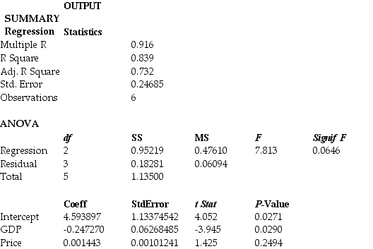 Note: Adj.R Square = Adjusted R Square;Std.Error = Standard Error
Referring to Instruction 13-14,the net regression coefficient of X2 is ________.
The Head of the Accounting Department wanted to see if she could predict the average grade of students using the number of course units (credits)and total university entrance exam scores of each.She takes a sample of students and generates the following Microsoft Excel output:
Note: Adj.R Square = Adjusted R Square;Std.Error = Standard ErrorReferring to Instruction 13-14,the net regression coefficient of X2 is ________.
سؤال
سؤال
Instruction 13-8
You worked as an intern at We Always Win Car Insurance Company last summer.You notice that individual car insurance premium depends very much on the age of the individual,the number of traffic tickets received by the individual,and the population density of the city in which the individual lives.You performed a regression analysis in Microsoft Excel and obtained the following information:
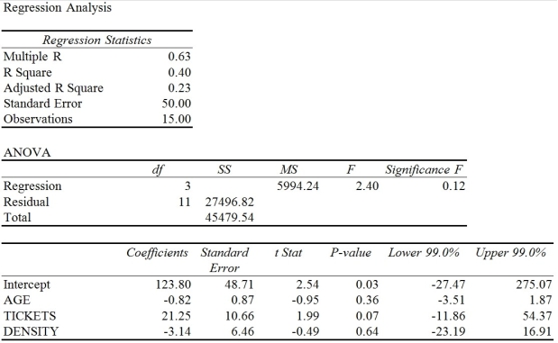
Referring to Instruction 13-8,the estimated mean change in insurance premiums for every two additional tickets received is ________.
You worked as an intern at We Always Win Car Insurance Company last summer.You notice that individual car insurance premium depends very much on the age of the individual,the number of traffic tickets received by the individual,and the population density of the city in which the individual lives.You performed a regression analysis in Microsoft Excel and obtained the following information:
Referring to Instruction 13-8,the estimated mean change in insurance premiums for every two additional tickets received is ________.
سؤال
Instruction 13-8
You worked as an intern at We Always Win Car Insurance Company last summer.You notice that individual car insurance premium depends very much on the age of the individual,the number of traffic tickets received by the individual,and the population density of the city in which the individual lives.You performed a regression analysis in Microsoft Excel and obtained the following information:
Referring to Instruction 13-8,the standard error of the estimate is ________.
سؤال
Instruction 13-8
You worked as an intern at We Always Win Car Insurance Company last summer.You notice that individual car insurance premium depends very much on the age of the individual,the number of traffic tickets received by the individual,and the population density of the city in which the individual lives.You performed a regression analysis in Microsoft Excel and obtained the following information:
Referring to Instruction 13-8,to test the significance of the multiple regression model,the value of the test statistic is ________.
سؤال
سؤال
Instruction 13-8
You worked as an intern at We Always Win Car Insurance Company last summer.You notice that individual car insurance premium depends very much on the age of the individual,the number of traffic tickets received by the individual,and the population density of the city in which the individual lives.You performed a regression analysis in Microsoft Excel and obtained the following information:
Referring to Instruction 13-8,the total degrees of freedom that are missing in the ANOVA table should be ________.
سؤال
Instruction 13-8
You worked as an intern at We Always Win Car Insurance Company last summer.You notice that individual car insurance premium depends very much on the age of the individual,the number of traffic tickets received by the individual,and the population density of the city in which the individual lives.You performed a regression analysis in Microsoft Excel and obtained the following information:
Referring to Instruction 13-8,to test the significance of the multiple regression model,the p-value of the test statistic in the sample is ________.
سؤال
Instruction 13-8
You worked as an intern at We Always Win Car Insurance Company last summer.You notice that individual car insurance premium depends very much on the age of the individual,the number of traffic tickets received by the individual,and the population density of the city in which the individual lives.You performed a regression analysis in Microsoft Excel and obtained the following information:
Referring to Instruction 13-8,the regression sum of squares that is missing in the ANOVA table should be ________.
سؤال
Instruction 13-8
You worked as an intern at We Always Win Car Insurance Company last summer.You notice that individual car insurance premium depends very much on the age of the individual,the number of traffic tickets received by the individual,and the population density of the city in which the individual lives.You performed a regression analysis in Microsoft Excel and obtained the following information:
Referring to Instruction 13-8,the adjusted r2 is ________.
سؤال
سؤال
Instruction 13-13
The education department's regional executive officer wanted to predict the percentage of students passing a Grade 6 proficiency test.She obtained the data on percentage of students passing the proficiency test (% Passing),daily average of the percentage of students attending class (% Attendance),average teacher salary in dollars (Salaries),and instructional spending per pupil in dollars (Spending)of 47 schools in the state.
Following is the multiple regression output with Y = % Passing as the dependent variable,
X1 = % Attendance,X2 = Salaries and X3 = Spending:
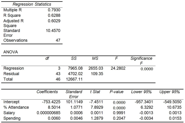
Referring to Instruction 13-13,predict the percentage of students passing the proficiency test for a school which has a daily mean of 95% of students attending class,an average teacher salary of 40,000 dollars,and an instructional spending per pupil of 2000 dollars.
The education department's regional executive officer wanted to predict the percentage of students passing a Grade 6 proficiency test.She obtained the data on percentage of students passing the proficiency test (% Passing),daily average of the percentage of students attending class (% Attendance),average teacher salary in dollars (Salaries),and instructional spending per pupil in dollars (Spending)of 47 schools in the state.
Following is the multiple regression output with Y = % Passing as the dependent variable,
X1 = % Attendance,X2 = Salaries and X3 = Spending:
Referring to Instruction 13-13,predict the percentage of students passing the proficiency test for a school which has a daily mean of 95% of students attending class,an average teacher salary of 40,000 dollars,and an instructional spending per pupil of 2000 dollars.
سؤال
سؤال
Instruction 13-8
You worked as an intern at We Always Win Car Insurance Company last summer.You notice that individual car insurance premium depends very much on the age of the individual,the number of traffic tickets received by the individual,and the population density of the city in which the individual lives.You performed a regression analysis in Microsoft Excel and obtained the following information:
Referring to Instruction 13-8,the proportion of the total variability in insurance premiums that can be explained by AGE,TICKETS,and DENSITY is ________.
سؤال
سؤال
Instruction 13-14
The Head of the Accounting Department wanted to see if she could predict the average grade of students using the number of course units (credits)and total university entrance exam scores of each.She takes a sample of students and generates the following Microsoft Excel output:
Note: Adj.R Square = Adjusted R Square;Std.Error = Standard Error
Referring to Instruction 13-14,the predicted mean grade for a student carrying 15 course units and who has a total university entrance exam score of 1,100 is ________.
The Head of the Accounting Department wanted to see if she could predict the average grade of students using the number of course units (credits)and total university entrance exam scores of each.She takes a sample of students and generates the following Microsoft Excel output:
Note: Adj.R Square = Adjusted R Square;Std.Error = Standard ErrorReferring to Instruction 13-14,the predicted mean grade for a student carrying 15 course units and who has a total university entrance exam score of 1,100 is ________.
سؤال
سؤال
Instruction 13-13
The education department's regional executive officer wanted to predict the percentage of students passing a Grade 6 proficiency test.She obtained the data on percentage of students passing the proficiency test (% Passing),daily average of the percentage of students attending class (% Attendance),average teacher salary in dollars (Salaries),and instructional spending per pupil in dollars (Spending)of 47 schools in the state.
Following is the multiple regression output with Y = % Passing as the dependent variable,
X1 = % Attendance,X2 = Salaries and X3 = Spending:
Referring to Instruction 13-13,estimate the mean percentage of students passing the proficiency test for all the schools that have a daily mean of 95% of students attending class,a mean teacher salary of 40,000 dollars,and an instructional spending per pupil of 2000 dollars.
سؤال
Instruction 13-14
The Head of the Accounting Department wanted to see if she could predict the average grade of students using the number of course units (credits)and total university entrance exam scores of each.She takes a sample of students and generates the following Microsoft Excel output:
Note: Adj.R Square = Adjusted R Square;Std.Error = Standard Error
Referring to Instruction 13-14,the estimate of the unit change in the mean of Y per unit change in X1,holding X2 constant,is ________.
The Head of the Accounting Department wanted to see if she could predict the average grade of students using the number of course units (credits)and total university entrance exam scores of each.She takes a sample of students and generates the following Microsoft Excel output:
Note: Adj.R Square = Adjusted R Square;Std.Error = Standard ErrorReferring to Instruction 13-14,the estimate of the unit change in the mean of Y per unit change in X1,holding X2 constant,is ________.
سؤال
سؤال
Instruction 13-15
A financial analyst wanted to examine the relationship between salary (in $1,000)and 4 variables: age (X1 = Age),experience in the field (X2 = Exper),number of degrees (X3 = Degrees),and number of previous jobs in the field (X4 = Prevjobs).He took a sample of 20 employees and obtained the following Microsoft Excel output:
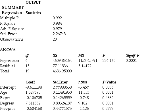 Note: Adj.R Square = Adjusted R Square;Std.Error = Standard Error
Referring to Instruction 13-15,the critical value of an F test on the entire regression for a level of significance of 0.01 is ________.
A financial analyst wanted to examine the relationship between salary (in $1,000)and 4 variables: age (X1 = Age),experience in the field (X2 = Exper),number of degrees (X3 = Degrees),and number of previous jobs in the field (X4 = Prevjobs).He took a sample of 20 employees and obtained the following Microsoft Excel output:
Note: Adj.R Square = Adjusted R Square;Std.Error = Standard ErrorReferring to Instruction 13-15,the critical value of an F test on the entire regression for a level of significance of 0.01 is ________.
سؤال
Instruction 13-14
The Head of the Accounting Department wanted to see if she could predict the average grade of students using the number of course units (credits)and total university entrance exam scores of each.She takes a sample of students and generates the following Microsoft Excel output:
Note: Adj.R Square = Adjusted R Square;Std.Error = Standard Error
Referring to Instruction 13-14,the Head of Department wants to test H0: β1 = β2 = 0.The appropriate alternative hypothesis is ________.
The Head of the Accounting Department wanted to see if she could predict the average grade of students using the number of course units (credits)and total university entrance exam scores of each.She takes a sample of students and generates the following Microsoft Excel output:
Note: Adj.R Square = Adjusted R Square;Std.Error = Standard ErrorReferring to Instruction 13-14,the Head of Department wants to test H0: β1 = β2 = 0.The appropriate alternative hypothesis is ________.
سؤال
Instruction 13-15
A financial analyst wanted to examine the relationship between salary (in $1,000)and 4 variables: age (X1 = Age),experience in the field (X2 = Exper),number of degrees (X3 = Degrees),and number of previous jobs in the field (X4 = Prevjobs).He took a sample of 20 employees and obtained the following Microsoft Excel output:
Note: Adj.R Square = Adjusted R Square;Std.Error = Standard Error
Referring to Instruction 13-15,the estimate of the unit change in the mean of Y per unit change in X4,taking into account the effects of the other three variables,is ________.
A financial analyst wanted to examine the relationship between salary (in $1,000)and 4 variables: age (X1 = Age),experience in the field (X2 = Exper),number of degrees (X3 = Degrees),and number of previous jobs in the field (X4 = Prevjobs).He took a sample of 20 employees and obtained the following Microsoft Excel output:
Note: Adj.R Square = Adjusted R Square;Std.Error = Standard ErrorReferring to Instruction 13-15,the estimate of the unit change in the mean of Y per unit change in X4,taking into account the effects of the other three variables,is ________.
سؤال
Instruction 13-14
The Head of the Accounting Department wanted to see if she could predict the average grade of students using the number of course units (credits)and total university entrance exam scores of each.She takes a sample of students and generates the following Microsoft Excel output:
Note: Adj.R Square = Adjusted R Square;Std.Error = Standard Error
Referring to Instruction 13-14,the value of the adjusted coefficient of multiple determination,r2adj,is ________.
The Head of the Accounting Department wanted to see if she could predict the average grade of students using the number of course units (credits)and total university entrance exam scores of each.She takes a sample of students and generates the following Microsoft Excel output:
Note: Adj.R Square = Adjusted R Square;Std.Error = Standard ErrorReferring to Instruction 13-14,the value of the adjusted coefficient of multiple determination,r2adj,is ________.
سؤال
Instruction 13-15
A financial analyst wanted to examine the relationship between salary (in $1,000)and 4 variables: age (X1 = Age),experience in the field (X2 = Exper),number of degrees (X3 = Degrees),and number of previous jobs in the field (X4 = Prevjobs).He took a sample of 20 employees and obtained the following Microsoft Excel output:
Note: Adj.R Square = Adjusted R Square;Std.Error = Standard Error
Referring to Instruction 13-15,the analyst wants to use an F test to test H0: β1 = β2 = β3 = β4 = 0.The appropriate alternative hypothesis is ________.
A financial analyst wanted to examine the relationship between salary (in $1,000)and 4 variables: age (X1 = Age),experience in the field (X2 = Exper),number of degrees (X3 = Degrees),and number of previous jobs in the field (X4 = Prevjobs).He took a sample of 20 employees and obtained the following Microsoft Excel output:
Note: Adj.R Square = Adjusted R Square;Std.Error = Standard ErrorReferring to Instruction 13-15,the analyst wants to use an F test to test H0: β1 = β2 = β3 = β4 = 0.The appropriate alternative hypothesis is ________.
سؤال
Instruction 13-16
Given below are results from the regression analysis where the dependent variable is the number of weeks a worker is unemployed due to a layoff (Unemploy)and the independent variables are the age of the worker (Age),the number of years of education received (Edu),the number of years at the previous job (Job Yr),a dummy variable for marital status (Married: 1 = married,0 = otherwise),a dummy variable for head of household (Head: 1 = yes,0 = no)and a dummy variable for management position (Manager: 1 = yes,0 = no).We shall call this Model 1.
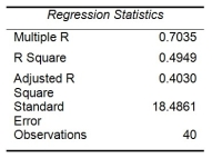
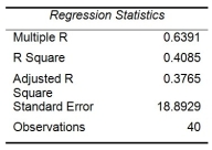
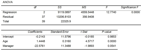
 Model 2 is the regression analysis where the dependent variable is Unemploy and the independent variables are Age and Manager.The results of the regression analysis are given below:
Referring to Instruction 13-16 Model 1,estimate the mean number of weeks being unemployed due to a layoff for a worker who is a 30 year old,has 10 years of education,has 15 years of experience at the previous job,is married,is the head of household,and is a manager.
Given below are results from the regression analysis where the dependent variable is the number of weeks a worker is unemployed due to a layoff (Unemploy)and the independent variables are the age of the worker (Age),the number of years of education received (Edu),the number of years at the previous job (Job Yr),a dummy variable for marital status (Married: 1 = married,0 = otherwise),a dummy variable for head of household (Head: 1 = yes,0 = no)and a dummy variable for management position (Manager: 1 = yes,0 = no).We shall call this Model 1.
Model 2 is the regression analysis where the dependent variable is Unemploy and the independent variables are Age and Manager.The results of the regression analysis are given below: Referring to Instruction 13-16 Model 1,estimate the mean number of weeks being unemployed due to a layoff for a worker who is a 30 year old,has 10 years of education,has 15 years of experience at the previous job,is married,is the head of household,and is a manager.
سؤال
Instruction 13-16
Given below are results from the regression analysis where the dependent variable is the number of weeks a worker is unemployed due to a layoff (Unemploy)and the independent variables are the age of the worker (Age),the number of years of education received (Edu),the number of years at the previous job (Job Yr),a dummy variable for marital status (Married: 1 = married,0 = otherwise),a dummy variable for head of household (Head: 1 = yes,0 = no)and a dummy variable for management position (Manager: 1 = yes,0 = no).We shall call this Model 1.
Model 2 is the regression analysis where the dependent variable is Unemploy and the independent variables are Age and Manager.The results of the regression analysis are given below:
Referring to Instruction 13-16 Model 1,predict the number of weeks being unemployed due to a layoff for a worker who is a 30 year old,has 10 years of education,has 15 years of experience at the previous job,is married,is the head of household,and is a manager.
Given below are results from the regression analysis where the dependent variable is the number of weeks a worker is unemployed due to a layoff (Unemploy)and the independent variables are the age of the worker (Age),the number of years of education received (Edu),the number of years at the previous job (Job Yr),a dummy variable for marital status (Married: 1 = married,0 = otherwise),a dummy variable for head of household (Head: 1 = yes,0 = no)and a dummy variable for management position (Manager: 1 = yes,0 = no).We shall call this Model 1.
Model 2 is the regression analysis where the dependent variable is Unemploy and the independent variables are Age and Manager.The results of the regression analysis are given below: Referring to Instruction 13-16 Model 1,predict the number of weeks being unemployed due to a layoff for a worker who is a 30 year old,has 10 years of education,has 15 years of experience at the previous job,is married,is the head of household,and is a manager.
سؤال
Instruction 13-15
A financial analyst wanted to examine the relationship between salary (in $1,000)and 4 variables: age (X1 = Age),experience in the field (X2 = Exper),number of degrees (X3 = Degrees),and number of previous jobs in the field (X4 = Prevjobs).He took a sample of 20 employees and obtained the following Microsoft Excel output:
Note: Adj.R Square = Adjusted R Square;Std.Error = Standard Error
Referring to Instruction 13-15,the predicted salary for a 35 year-old person with 10 years of experience,3 degrees,and 1 previous job is ________.
A financial analyst wanted to examine the relationship between salary (in $1,000)and 4 variables: age (X1 = Age),experience in the field (X2 = Exper),number of degrees (X3 = Degrees),and number of previous jobs in the field (X4 = Prevjobs).He took a sample of 20 employees and obtained the following Microsoft Excel output:
Note: Adj.R Square = Adjusted R Square;Std.Error = Standard ErrorReferring to Instruction 13-15,the predicted salary for a 35 year-old person with 10 years of experience,3 degrees,and 1 previous job is ________.
سؤال
Instruction 13-14
The Head of the Accounting Department wanted to see if she could predict the average grade of students using the number of course units (credits)and total university entrance exam scores of each.She takes a sample of students and generates the following Microsoft Excel output:
Note: Adj.R Square = Adjusted R Square;Std.Error = Standard Error
Referring to Instruction 13-14,the Head of Department wants to test H0: β1 = β2 = 0.The critical value of the F test for a level of significance of 0.05 is ________.
The Head of the Accounting Department wanted to see if she could predict the average grade of students using the number of course units (credits)and total university entrance exam scores of each.She takes a sample of students and generates the following Microsoft Excel output:
Note: Adj.R Square = Adjusted R Square;Std.Error = Standard ErrorReferring to Instruction 13-14,the Head of Department wants to test H0: β1 = β2 = 0.The critical value of the F test for a level of significance of 0.05 is ________.
سؤال
Instruction 13-14
The Head of the Accounting Department wanted to see if she could predict the average grade of students using the number of course units (credits)and total university entrance exam scores of each.She takes a sample of students and generates the following Microsoft Excel output:
Note: Adj.R Square = Adjusted R Square;Std.Error = Standard Error
Referring to Instruction 13-14,the Head of Department wants to test H0: β1 = β2 = 0.The p-value of the test is ________.
The Head of the Accounting Department wanted to see if she could predict the average grade of students using the number of course units (credits)and total university entrance exam scores of each.She takes a sample of students and generates the following Microsoft Excel output:
Note: Adj.R Square = Adjusted R Square;Std.Error = Standard ErrorReferring to Instruction 13-14,the Head of Department wants to test H0: β1 = β2 = 0.The p-value of the test is ________.
سؤال
Instruction 13-15
A financial analyst wanted to examine the relationship between salary (in $1,000)and 4 variables: age (X1 = Age),experience in the field (X2 = Exper),number of degrees (X3 = Degrees),and number of previous jobs in the field (X4 = Prevjobs).He took a sample of 20 employees and obtained the following Microsoft Excel output:
Note: Adj.R Square = Adjusted R Square;Std.Error = Standard Error
Referring to Instruction 13-15,the value of the coefficient of multiple determination,r2Y.1234,is ________.
A financial analyst wanted to examine the relationship between salary (in $1,000)and 4 variables: age (X1 = Age),experience in the field (X2 = Exper),number of degrees (X3 = Degrees),and number of previous jobs in the field (X4 = Prevjobs).He took a sample of 20 employees and obtained the following Microsoft Excel output:
Note: Adj.R Square = Adjusted R Square;Std.Error = Standard ErrorReferring to Instruction 13-15,the value of the coefficient of multiple determination,r2Y.1234,is ________.
سؤال
Instruction 13-14
The Head of the Accounting Department wanted to see if she could predict the average grade of students using the number of course units (credits)and total university entrance exam scores of each.She takes a sample of students and generates the following Microsoft Excel output:
Note: Adj.R Square = Adjusted R Square;Std.Error = Standard Error
Referring to Instruction 13-14,the Head of Department wants to test H0: β1 = β2 = 0.The value of the F test statistic is ________.
The Head of the Accounting Department wanted to see if she could predict the average grade of students using the number of course units (credits)and total university entrance exam scores of each.She takes a sample of students and generates the following Microsoft Excel output:
Note: Adj.R Square = Adjusted R Square;Std.Error = Standard ErrorReferring to Instruction 13-14,the Head of Department wants to test H0: β1 = β2 = 0.The value of the F test statistic is ________.
سؤال
سؤال
Instruction 13-14
The Head of the Accounting Department wanted to see if she could predict the average grade of students using the number of course units (credits)and total university entrance exam scores of each.She takes a sample of students and generates the following Microsoft Excel output:
Note: Adj.R Square = Adjusted R Square;Std.Error = Standard Error
Referring to Instruction 13-14,the value of the coefficient of multiple determination,r2Y.12,is ________.
The Head of the Accounting Department wanted to see if she could predict the average grade of students using the number of course units (credits)and total university entrance exam scores of each.She takes a sample of students and generates the following Microsoft Excel output:
Note: Adj.R Square = Adjusted R Square;Std.Error = Standard ErrorReferring to Instruction 13-14,the value of the coefficient of multiple determination,r2Y.12,is ________.
سؤال
Instruction 13-15
A financial analyst wanted to examine the relationship between salary (in $1,000)and 4 variables: age (X1 = Age),experience in the field (X2 = Exper),number of degrees (X3 = Degrees),and number of previous jobs in the field (X4 = Prevjobs).He took a sample of 20 employees and obtained the following Microsoft Excel output:
Note: Adj.R Square = Adjusted R Square;Std.Error = Standard Error
Referring to Instruction 13-15,the value of the F statistic for testing the significance of the entire regression is ________.
A financial analyst wanted to examine the relationship between salary (in $1,000)and 4 variables: age (X1 = Age),experience in the field (X2 = Exper),number of degrees (X3 = Degrees),and number of previous jobs in the field (X4 = Prevjobs).He took a sample of 20 employees and obtained the following Microsoft Excel output:
Note: Adj.R Square = Adjusted R Square;Std.Error = Standard ErrorReferring to Instruction 13-15,the value of the F statistic for testing the significance of the entire regression is ________.
سؤال
Instruction 13-15
A financial analyst wanted to examine the relationship between salary (in $1,000)and 4 variables: age (X1 = Age),experience in the field (X2 = Exper),number of degrees (X3 = Degrees),and number of previous jobs in the field (X4 = Prevjobs).He took a sample of 20 employees and obtained the following Microsoft Excel output:
Note: Adj.R Square = Adjusted R Square;Std.Error = Standard Error
Referring to Instruction 13-15,the p-value of the F test for the significance of the entire regression is ________.
A financial analyst wanted to examine the relationship between salary (in $1,000)and 4 variables: age (X1 = Age),experience in the field (X2 = Exper),number of degrees (X3 = Degrees),and number of previous jobs in the field (X4 = Prevjobs).He took a sample of 20 employees and obtained the following Microsoft Excel output:
Note: Adj.R Square = Adjusted R Square;Std.Error = Standard ErrorReferring to Instruction 13-15,the p-value of the F test for the significance of the entire regression is ________.
سؤال
سؤال
سؤال
Instruction 13-15
A financial analyst wanted to examine the relationship between salary (in $1,000)and 4 variables: age (X1 = Age),experience in the field (X2 = Exper),number of degrees (X3 = Degrees),and number of previous jobs in the field (X4 = Prevjobs).He took a sample of 20 employees and obtained the following Microsoft Excel output:
Note: Adj.R Square = Adjusted R Square;Std.Error = Standard Error
Referring to Instruction 13-15,the net regression coefficient of X2 is ________.
A financial analyst wanted to examine the relationship between salary (in $1,000)and 4 variables: age (X1 = Age),experience in the field (X2 = Exper),number of degrees (X3 = Degrees),and number of previous jobs in the field (X4 = Prevjobs).He took a sample of 20 employees and obtained the following Microsoft Excel output:
Note: Adj.R Square = Adjusted R Square;Std.Error = Standard ErrorReferring to Instruction 13-15,the net regression coefficient of X2 is ________.
سؤال
Instruction 13-15
A financial analyst wanted to examine the relationship between salary (in $1,000)and 4 variables: age (X1 = Age),experience in the field (X2 = Exper),number of degrees (X3 = Degrees),and number of previous jobs in the field (X4 = Prevjobs).He took a sample of 20 employees and obtained the following Microsoft Excel output:
Note: Adj.R Square = Adjusted R Square;Std.Error = Standard Error
Referring to Instruction 13-15,the value of the adjusted coefficient of multiple determination,adjusted r2,is ________.
A financial analyst wanted to examine the relationship between salary (in $1,000)and 4 variables: age (X1 = Age),experience in the field (X2 = Exper),number of degrees (X3 = Degrees),and number of previous jobs in the field (X4 = Prevjobs).He took a sample of 20 employees and obtained the following Microsoft Excel output:
Note: Adj.R Square = Adjusted R Square;Std.Error = Standard ErrorReferring to Instruction 13-15,the value of the adjusted coefficient of multiple determination,adjusted r2,is ________.
سؤال
سؤال
سؤال
سؤال
سؤال
سؤال
سؤال
سؤال
سؤال
سؤال
سؤال
سؤال
سؤال
سؤال
سؤال
سؤال
سؤال
سؤال
سؤال
سؤال

فتح الحزمة
قم بالتسجيل لفتح البطاقات في هذه المجموعة!
Unlock Deck
Unlock Deck
1/256
العب
ملء الشاشة (f)
Deck 13: Introduction to Multiple Regression
1
Instruction 13-3
An economist is interested to see how consumption for an economy (in $ billions)is influenced by gross domestic product ($ billions)and aggregate price (consumer price index).The Microsoft Excel output of this regression is partially reproduced below.
OUTPUT
SUMMARY
Regression Statistics
ANOVA
Note: Adj.R Square = Adjusted R Square;Std.Error = Standard Error
-Referring to Instruction 13-3,what is the estimated average consumption level for an economy with GDP equal to $4 billion and an aggregate price index of 150?
A)$1.39 billion.
B)$2.89 billion.
C)$4.75 billion.
D)$9.45 billion.
$2.89 billion.
2
A multiple regression is called "multiple" because it has several explanatory variables.
True
3
Instruction 13-3
An economist is interested to see how consumption for an economy (in $ billions)is influenced by gross domestic product ($ billions)and aggregate price (consumer price index).The Microsoft Excel output of this regression is partially reproduced below.
OUTPUT
SUMMARY
Regression Statistics
ANOVA
Note: Adj.R Square = Adjusted R Square;Std.Error = Standard Error
-Referring to Instruction 13-3,what is the estimated average consumption level for an economy with GDP equal to $2 billion and an aggregate price index of 90?
A)$1.39 billion.
B)$2.89 billion.
C)$4.75 billion.
D)$9.45 billion.
$1.39 billion.
4
Instruction 13-1
A manager of a product sales group believes the number of sales made by an employee (Y)depends on how many years that employee has been with the company (X1)and how he/she scored on a business aptitude test (X2).A random sample of 8 employees provides the following:
-Referring to Instruction 13-1,for these data,what is the estimated coefficient for the variable representing years an employee has been with the company,b1?
A)3.103
B)4.698
C)21.293
D)0.998
فتح الحزمة
افتح القفل للوصول البطاقات البالغ عددها 256 في هذه المجموعة.
فتح الحزمة
k this deck
5
Instruction 13-3
An economist is interested to see how consumption for an economy (in $ billions)is influenced by gross domestic product ($ billions)and aggregate price (consumer price index).The Microsoft Excel output of this regression is partially reproduced below.
OUTPUT
SUMMARY
Regression Statistics
ANOVA
Note: Adj.R Square = Adjusted R Square;Std.Error = Standard Error
-Referring to Instruction 13-3,the p-value for the regression model as a whole is
A)0.01.
B)0.001.
C)0.05.
D)None of the above.
فتح الحزمة
افتح القفل للوصول البطاقات البالغ عددها 256 في هذه المجموعة.
فتح الحزمة
k this deck
6
Instruction 13-1
A manager of a product sales group believes the number of sales made by an employee (Y)depends on how many years that employee has been with the company (X1)and how he/she scored on a business aptitude test (X2).A random sample of 8 employees provides the following:
-Referring to Instruction 13-1,for these data,what is the value for the regression constant,b0?
A)0.998
B)21.293
C)3.103
D)4.698
فتح الحزمة
افتح القفل للوصول البطاقات البالغ عددها 256 في هذه المجموعة.
فتح الحزمة
k this deck
7
Instruction 13-1
A manager of a product sales group believes the number of sales made by an employee (Y)depends on how many years that employee has been with the company (X1)and how he/she scored on a business aptitude test (X2).A random sample of 8 employees provides the following:
-Referring to Instruction 13-1,for these data,what is the estimated coefficient for the variable representing scores on the aptitude test,b2?
A)21.293
B)0.998
C)3.103
D)4.698
فتح الحزمة
افتح القفل للوصول البطاقات البالغ عددها 256 في هذه المجموعة.
فتح الحزمة
k this deck
8
Instruction 13-2
A lecturer in industrial relations believes that an individual's wage rate at a factory (Y)depends on his performance rating (X1)and the number of economics courses the employee successfully completed at university (X2).The lecturer randomly selects six workers and collects the following information:
-Referring to Instruction 13-2,an employee who took 12 economics courses scores 10 on the performance rating.What is her estimated expected wage rate?
A)$25.70
B)$10.90
C)$24.87
D)$12.20
فتح الحزمة
افتح القفل للوصول البطاقات البالغ عددها 256 في هذه المجموعة.
فتح الحزمة
k this deck
9
Instruction 13-2
A lecturer in industrial relations believes that an individual's wage rate at a factory (Y)depends on his performance rating (X1)and the number of economics courses the employee successfully completed at university (X2).The lecturer randomly selects six workers and collects the following information:
-Referring to Instruction 13-2,for these data,what is the value for the regression constant,b0?
A)9.103
B)6.932
C)1.054
D)0.616
فتح الحزمة
افتح القفل للوصول البطاقات البالغ عددها 256 في هذه المجموعة.
فتح الحزمة
k this deck
10
Instruction 13-1
A manager of a product sales group believes the number of sales made by an employee (Y)depends on how many years that employee has been with the company (X1)and how he/she scored on a business aptitude test (X2).A random sample of 8 employees provides the following:
-Referring to Instruction 13-1,if an employee who had been with the company five years scored a 9 on the aptitude test,what would his estimated expected sales be?
A)60.88
B)17.98
C)55.62
D)79.09
فتح الحزمة
افتح القفل للوصول البطاقات البالغ عددها 256 في هذه المجموعة.
فتح الحزمة
k this deck
11
Multiple regression is the process of using several independent variables to predict a number of dependent variables.
فتح الحزمة
افتح القفل للوصول البطاقات البالغ عددها 256 في هذه المجموعة.
فتح الحزمة
k this deck
12
The interpretation of the slope is different in a multiple linear regression model as compared to a simple linear regression model.
فتح الحزمة
افتح القفل للوصول البطاقات البالغ عددها 256 في هذه المجموعة.
فتح الحزمة
k this deck
13
Instruction 13-4
A real estate builder wishes to determine how house size (House)is influenced by family income (Income),family size (Size),and education of the head of household (School).House size is measured in hundreds of square metres,income is measured in thousands of dollars,and education is in years.The builder randomly selected 50 families and ran the multiple regression.Microsoft Excel output is provided below:
SUMMARY
Regression Statistics
ANOVA
Note: Adj.R Square = Adjusted R Square;Std.Error = Standard Error
-Referring to Instruction 13-4,what minimum annual income would an individual with a family size of 9 and 10 years of education need to attain a predicted 5,000 square metre home (House = 50)?
A)$56.75 thousand.
B)$211.85 thousand.
C)$178.33 thousand.
D)$44.14 thousand.
فتح الحزمة
افتح القفل للوصول البطاقات البالغ عددها 256 في هذه المجموعة.
فتح الحزمة
k this deck
14
Instruction 13-3
An economist is interested to see how consumption for an economy (in $ billions)is influenced by gross domestic product ($ billions)and aggregate price (consumer price index).The Microsoft Excel output of this regression is partially reproduced below.
OUTPUT
SUMMARY
Regression Statistics
ANOVA
Note: Adj.R Square = Adjusted R Square;Std.Error = Standard Error
-Referring to Instruction 13-3,what is the predicted consumption level for an economy with GDP equal to $4 billion and an aggregate price index of 150?
A)$1.39 billion.
B)$2.89 billion.
C)$4.75 billion.
D)$9.45 billion.
فتح الحزمة
افتح القفل للوصول البطاقات البالغ عددها 256 في هذه المجموعة.
فتح الحزمة
k this deck
15
Instruction 13-4
A real estate builder wishes to determine how house size (House)is influenced by family income (Income),family size (Size),and education of the head of household (School).House size is measured in hundreds of square metres,income is measured in thousands of dollars,and education is in years.The builder randomly selected 50 families and ran the multiple regression.Microsoft Excel output is provided below:
SUMMARY
Regression Statistics
ANOVA
Note: Adj.R Square = Adjusted R Square;Std.Error = Standard Error
-Referring to Instruction 13-4,what minimum annual income would an individual with a family size of 4 and 16 years of education need to attain a predicted 10,000 square metre home (House = 100)?
A)$178.33 thousand.
B)$211.85 thousand.
C)$44.14 thousand.
D)$56.75 thousand.
فتح الحزمة
افتح القفل للوصول البطاقات البالغ عددها 256 في هذه المجموعة.
فتح الحزمة
k this deck
16
A multiple regression is called "multiple" because it has several data points.
فتح الحزمة
افتح القفل للوصول البطاقات البالغ عددها 256 في هذه المجموعة.
فتح الحزمة
k this deck
17
Instruction 13-2
A lecturer in industrial relations believes that an individual's wage rate at a factory (Y)depends on his performance rating (X1)and the number of economics courses the employee successfully completed at university (X2).The lecturer randomly selects six workers and collects the following information:
-Referring to Instruction 13-2,for these data,what is the estimated coefficient for the number of economics courses taken,b2?
A)6.932
B)1.054
C)9.103
D)0.616
فتح الحزمة
افتح القفل للوصول البطاقات البالغ عددها 256 في هذه المجموعة.
فتح الحزمة
k this deck
18
Instruction 13-2
A lecturer in industrial relations believes that an individual's wage rate at a factory (Y)depends on his performance rating (X1)and the number of economics courses the employee successfully completed at university (X2).The lecturer randomly selects six workers and collects the following information:
-Referring to Instruction 13-2,suppose an employee had never taken an economics course and managed to score a 5 on his performance rating.What is his estimated expected wage rate?
A)$12.20
B)$25.11
C)$10.90
D)$17.23
فتح الحزمة
افتح القفل للوصول البطاقات البالغ عددها 256 في هذه المجموعة.
فتح الحزمة
k this deck
19
In a multiple regression problem involving two independent variables,if b1 is computed to be +2.0,it means that
A)the estimated mean of Y increases by 2 units for each increase of 1 unit of X1,without regard to X2.
B)the estimated mean of Y increases by 2 units for each increase of 1 unit of X1,holding X2 constant.
C)the estimated mean of Y is 2 when X1 equals zero.
D)the relationship between X1 and Y is significant.
فتح الحزمة
افتح القفل للوصول البطاقات البالغ عددها 256 في هذه المجموعة.
فتح الحزمة
k this deck
20
Instruction 13-2
A lecturer in industrial relations believes that an individual's wage rate at a factory (Y)depends on his performance rating (X1)and the number of economics courses the employee successfully completed at university (X2).The lecturer randomly selects six workers and collects the following information:
-Referring to Instruction 13-2,for these data,what is the estimated coefficient for performance rating,b1?
A)9.103
B)0.616
C)6.932
D)1.054
فتح الحزمة
افتح القفل للوصول البطاقات البالغ عددها 256 في هذه المجموعة.
فتح الحزمة
k this deck
21
Instruction 13-14
The Head of the Accounting Department wanted to see if she could predict the average grade of students using the number of course units (credits)and total university entrance exam scores of each.She takes a sample of students and generates the following Microsoft Excel output:
Note: Adj.R Square = Adjusted R Square;Std.Error = Standard Error
Referring to Instruction 13-14,the net regression coefficient of X2 is ________.
The Head of the Accounting Department wanted to see if she could predict the average grade of students using the number of course units (credits)and total university entrance exam scores of each.She takes a sample of students and generates the following Microsoft Excel output:
Note: Adj.R Square = Adjusted R Square;Std.Error = Standard ErrorReferring to Instruction 13-14,the net regression coefficient of X2 is ________.
فتح الحزمة
افتح القفل للوصول البطاقات البالغ عددها 256 في هذه المجموعة.
فتح الحزمة
k this deck
22
Instruction 13-4
A real estate builder wishes to determine how house size (House)is influenced by family income (Income),family size (Size),and education of the head of household (School).House size is measured in hundreds of square metres,income is measured in thousands of dollars,and education is in years.The builder randomly selected 50 families and ran the multiple regression.Microsoft Excel output is provided below:
SUMMARY
Regression Statistics
ANOVA
Note: Adj.R Square = Adjusted R Square;Std.Error = Standard Error
-Referring to Instruction 13-4,what is the predicted house size (in hundreds of square metres)for an individual earning an annual income of $40,000,having a family size of 4,and going to school a total of 13 years?
A)15.15
B)53.87
C)11.43
D)24.88
فتح الحزمة
افتح القفل للوصول البطاقات البالغ عددها 256 في هذه المجموعة.
فتح الحزمة
k this deck
23
Instruction 13-8
You worked as an intern at We Always Win Car Insurance Company last summer.You notice that individual car insurance premium depends very much on the age of the individual,the number of traffic tickets received by the individual,and the population density of the city in which the individual lives.You performed a regression analysis in Microsoft Excel and obtained the following information:
Referring to Instruction 13-8,the estimated mean change in insurance premiums for every two additional tickets received is ________.
فتح الحزمة
افتح القفل للوصول البطاقات البالغ عددها 256 في هذه المجموعة.
فتح الحزمة
k this deck
24
Instruction 13-8
You worked as an intern at We Always Win Car Insurance Company last summer.You notice that individual car insurance premium depends very much on the age of the individual,the number of traffic tickets received by the individual,and the population density of the city in which the individual lives.You performed a regression analysis in Microsoft Excel and obtained the following information:
Referring to Instruction 13-8,the standard error of the estimate is ________.
فتح الحزمة
افتح القفل للوصول البطاقات البالغ عددها 256 في هذه المجموعة.
فتح الحزمة
k this deck
25
Instruction 13-8
You worked as an intern at We Always Win Car Insurance Company last summer.You notice that individual car insurance premium depends very much on the age of the individual,the number of traffic tickets received by the individual,and the population density of the city in which the individual lives.You performed a regression analysis in Microsoft Excel and obtained the following information:
Referring to Instruction 13-8,to test the significance of the multiple regression model,the value of the test statistic is ________.
فتح الحزمة
افتح القفل للوصول البطاقات البالغ عددها 256 في هذه المجموعة.
فتح الحزمة
k this deck
26
Instruction 13-10
As a project for his business statistics class,a student examined the factors that determined parking meter rates throughout the campus area.Data were collected for the price per hour of parking,number of city blocks to the centre of the university,and one of the three jurisdictions: on campus,in the CBD and off campus,or outside of the CBD and off campus.The population regression model hypothesised is:
Yi = ? + ?1x1i + ?2x2i + ?3x2i + ?i
Where
Y is the meter price
x1 is the number of blocks to the centre of the university
x2 is a dummy variable that takes the value 1 if the meter is located in the CBD and off campus and the value 0 otherwise
x3 is a dummy variable that takes the value 1 if the meter is located outside of the CBD and off campus,and the value 0 otherwise
The following Excel results are obtained.
ANOVA
-Referring to Instruction 13-10,predict the meter rate per hour if one parks outside of the CBD and off campus three blocks from the centre of the university.
A)$0.4981
B)$0.2589
C)$0.0139
D)$0.2604
فتح الحزمة
افتح القفل للوصول البطاقات البالغ عددها 256 في هذه المجموعة.
فتح الحزمة
k this deck
27
Instruction 13-8
You worked as an intern at We Always Win Car Insurance Company last summer.You notice that individual car insurance premium depends very much on the age of the individual,the number of traffic tickets received by the individual,and the population density of the city in which the individual lives.You performed a regression analysis in Microsoft Excel and obtained the following information:
Referring to Instruction 13-8,the total degrees of freedom that are missing in the ANOVA table should be ________.
فتح الحزمة
افتح القفل للوصول البطاقات البالغ عددها 256 في هذه المجموعة.
فتح الحزمة
k this deck
28
Instruction 13-8
You worked as an intern at We Always Win Car Insurance Company last summer.You notice that individual car insurance premium depends very much on the age of the individual,the number of traffic tickets received by the individual,and the population density of the city in which the individual lives.You performed a regression analysis in Microsoft Excel and obtained the following information:
Referring to Instruction 13-8,to test the significance of the multiple regression model,the p-value of the test statistic in the sample is ________.
فتح الحزمة
افتح القفل للوصول البطاقات البالغ عددها 256 في هذه المجموعة.
فتح الحزمة
k this deck
29
Instruction 13-8
You worked as an intern at We Always Win Car Insurance Company last summer.You notice that individual car insurance premium depends very much on the age of the individual,the number of traffic tickets received by the individual,and the population density of the city in which the individual lives.You performed a regression analysis in Microsoft Excel and obtained the following information:
Referring to Instruction 13-8,the regression sum of squares that is missing in the ANOVA table should be ________.
فتح الحزمة
افتح القفل للوصول البطاقات البالغ عددها 256 في هذه المجموعة.
فتح الحزمة
k this deck
30
Instruction 13-8
You worked as an intern at We Always Win Car Insurance Company last summer.You notice that individual car insurance premium depends very much on the age of the individual,the number of traffic tickets received by the individual,and the population density of the city in which the individual lives.You performed a regression analysis in Microsoft Excel and obtained the following information:
Referring to Instruction 13-8,the adjusted r2 is ________.
فتح الحزمة
افتح القفل للوصول البطاقات البالغ عددها 256 في هذه المجموعة.
فتح الحزمة
k this deck
31
Instruction 13-5
A microeconomist wants to determine how corporate sales are influenced by capital and wage spending by companies.She proceeds to randomly select 26 large corporations and record information in millions of dollars.The Microsoft Excel output below shows results of this multiple regression.
SUMMARY
Regression Statistics
Multiple R
R Square
Adj. R Square
Std. Error
Observations
ANOVA
Note: Adj.R Square = Adjusted R Square;Std.Error = Standard Error
-Referring to Instruction 13-5,what are the predicted sales (in millions of dollars)for a company spending $500 million on capital and $200 million on wages?
A)17,277.49
B)15,800.00
C)16,520.07
D)20,455.98
فتح الحزمة
افتح القفل للوصول البطاقات البالغ عددها 256 في هذه المجموعة.
فتح الحزمة
k this deck
32
Instruction 13-13
The education department's regional executive officer wanted to predict the percentage of students passing a Grade 6 proficiency test.She obtained the data on percentage of students passing the proficiency test (% Passing),daily average of the percentage of students attending class (% Attendance),average teacher salary in dollars (Salaries),and instructional spending per pupil in dollars (Spending)of 47 schools in the state.
Following is the multiple regression output with Y = % Passing as the dependent variable,
X1 = % Attendance,X2 = Salaries and X3 = Spending:
Referring to Instruction 13-13,predict the percentage of students passing the proficiency test for a school which has a daily mean of 95% of students attending class,an average teacher salary of 40,000 dollars,and an instructional spending per pupil of 2000 dollars.
فتح الحزمة
افتح القفل للوصول البطاقات البالغ عددها 256 في هذه المجموعة.
فتح الحزمة
k this deck
33
Instruction 13-6
One of the most common questions of prospective house buyers pertains to the average cost of heating in dollars (Y).
To provide its customers with information on that matter,a large real estate firm used the following 4 variables to predict heating costs: the daily minimum outside temperature in degrees of Celsius (X1),the amount of insulation in cm (X2),the number of windows in the house (X3),and the age of the furnace in years (X4).Given below are the Microsoft Excel outputs of two regression models.
ANOVA
ANOVA
-Referring to Instruction 13-6,the estimated value of the partial regression parameter ?1 in Model 1 means that
A)holding the effect of the other independent variables constant,an estimated expected $1 increase in heating costs is associated with a decrease in the daily minimum outside temperature by 4.51 degrees.
B)holding the effect of the other independent variables constant,a 1% increase in the daily minimum outside temperature results in an estimated expected decrease in heating costs by 4.51%.
C)holding the effect of the other independent variables constant,a 1 degree increase in the daily minimum outside temperature results in a decrease in heating costs by $4.51.
D)holding the effect of the other independent variables constant,a 1 degree increase in the daily minimum outside temperature results in an estimated expected decrease in heating costs by $4.51.
فتح الحزمة
افتح القفل للوصول البطاقات البالغ عددها 256 في هذه المجموعة.
فتح الحزمة
k this deck
34
Instruction 13-8
You worked as an intern at We Always Win Car Insurance Company last summer.You notice that individual car insurance premium depends very much on the age of the individual,the number of traffic tickets received by the individual,and the population density of the city in which the individual lives.You performed a regression analysis in Microsoft Excel and obtained the following information:
Referring to Instruction 13-8,the proportion of the total variability in insurance premiums that can be explained by AGE,TICKETS,and DENSITY is ________.
فتح الحزمة
افتح القفل للوصول البطاقات البالغ عددها 256 في هذه المجموعة.
فتح الحزمة
k this deck
35
Instruction 13-5
A microeconomist wants to determine how corporate sales are influenced by capital and wage spending by companies.She proceeds to randomly select 26 large corporations and record information in millions of dollars.The Microsoft Excel output below shows results of this multiple regression.
SUMMARY
Regression Statistics
Multiple R
R Square
Adj. R Square
Std. Error
Observations
ANOVA
Note: Adj.R Square = Adjusted R Square;Std.Error = Standard Error
-Referring to Instruction 13-5,what are the predicted sales (in millions of dollars)for a company spending $100 million on capital and $100 million on wages?
A)20,455.98
B)17,277.49
C)16,520.07
D)15,800.00
فتح الحزمة
افتح القفل للوصول البطاقات البالغ عددها 256 في هذه المجموعة.
فتح الحزمة
k this deck
36
Instruction 13-14
The Head of the Accounting Department wanted to see if she could predict the average grade of students using the number of course units (credits)and total university entrance exam scores of each.She takes a sample of students and generates the following Microsoft Excel output:
Note: Adj.R Square = Adjusted R Square;Std.Error = Standard Error
Referring to Instruction 13-14,the predicted mean grade for a student carrying 15 course units and who has a total university entrance exam score of 1,100 is ________.
The Head of the Accounting Department wanted to see if she could predict the average grade of students using the number of course units (credits)and total university entrance exam scores of each.She takes a sample of students and generates the following Microsoft Excel output:
Note: Adj.R Square = Adjusted R Square;Std.Error = Standard ErrorReferring to Instruction 13-14,the predicted mean grade for a student carrying 15 course units and who has a total university entrance exam score of 1,100 is ________.
فتح الحزمة
افتح القفل للوصول البطاقات البالغ عددها 256 في هذه المجموعة.
فتح الحزمة
k this deck
37
Instruction 13-13
The education department's regional executive officer wanted to predict the percentage of students passing a Grade 6 proficiency test.She obtained the data on percentage of students passing the proficiency test (% Passing),daily average of the percentage of students attending class (% Attendance),average teacher salary in dollars (Salaries),and instructional spending per pupil in dollars (Spending)of 47 schools in the state.
Following is the multiple regression output with Y = % Passing as the dependent variable,
X1 = % Attendance,X2 = Salaries and X3 = Spending:
ANOVA
-Referring to Instruction 13-13,which of the following is a correct statement?
A)The daily mean of the percentage of students attending class is expected to go up by an estimated 8.50% when the percentage of students passing the proficiency test increases by 1% holding constant the effects of all the remaining independent variables.
B)The mean percentage of students passing the proficiency test is estimated to go up by 8.50% when daily mean of percentage of students attending class increases by 1%.
C)The daily mean of the percentage of students attending class is expected to go up by an estimated 8.50% when the percentage of students passing the proficiency test increases by 1%.
D)The mean percentage of students passing the proficiency test is estimated to go up by 8.50% when daily mean of the percentage of students attending class increases by 1% holding constant the effects of all the remaining independent variables.
فتح الحزمة
افتح القفل للوصول البطاقات البالغ عددها 256 في هذه المجموعة.
فتح الحزمة
k this deck
38
Instruction 13-13
The education department's regional executive officer wanted to predict the percentage of students passing a Grade 6 proficiency test.She obtained the data on percentage of students passing the proficiency test (% Passing),daily average of the percentage of students attending class (% Attendance),average teacher salary in dollars (Salaries),and instructional spending per pupil in dollars (Spending)of 47 schools in the state.
Following is the multiple regression output with Y = % Passing as the dependent variable,
X1 = % Attendance,X2 = Salaries and X3 = Spending:
Referring to Instruction 13-13,estimate the mean percentage of students passing the proficiency test for all the schools that have a daily mean of 95% of students attending class,a mean teacher salary of 40,000 dollars,and an instructional spending per pupil of 2000 dollars.
فتح الحزمة
افتح القفل للوصول البطاقات البالغ عددها 256 في هذه المجموعة.
فتح الحزمة
k this deck
39
Instruction 13-14
The Head of the Accounting Department wanted to see if she could predict the average grade of students using the number of course units (credits)and total university entrance exam scores of each.She takes a sample of students and generates the following Microsoft Excel output:
Note: Adj.R Square = Adjusted R Square;Std.Error = Standard Error
Referring to Instruction 13-14,the estimate of the unit change in the mean of Y per unit change in X1,holding X2 constant,is ________.
The Head of the Accounting Department wanted to see if she could predict the average grade of students using the number of course units (credits)and total university entrance exam scores of each.She takes a sample of students and generates the following Microsoft Excel output:
Note: Adj.R Square = Adjusted R Square;Std.Error = Standard ErrorReferring to Instruction 13-14,the estimate of the unit change in the mean of Y per unit change in X1,holding X2 constant,is ________.
فتح الحزمة
افتح القفل للوصول البطاقات البالغ عددها 256 في هذه المجموعة.
فتح الحزمة
k this deck
40
Instruction 13-9
A weight-loss clinic wants to use regression analysis to build a model for weight-loss of a client (measured in kilograms).Two variables thought to effect weight-loss are client's length of time on the weight loss program and time of session.These variables are described below:
Y = Weight-loss (in kilograms)
X1 = Length of time in weight-loss program (in months)
X2 = 1 if morning session,0 if not
X3 = 1 if afternoon session,0 if not (Base level = evening session)
Data for 12 clients on a weight-loss program at the clinic were collected and used to fit the interaction model:
Y = ?0 + ?1X1 + ?2X2 + ?3X3 + ?4X1X2 + ?5X1X3 + ?
Partial output from Microsoft Excel follows:
Regression Statistics
ANOVA
-Referring to Instruction 13-9,what is the experimental unit for this analysis?
A)A client on a weight-loss program.
B)A month.
C)A morning,afternoon,or evening session.
D)A clinic.
فتح الحزمة
افتح القفل للوصول البطاقات البالغ عددها 256 في هذه المجموعة.
فتح الحزمة
k this deck
41
Instruction 13-15
A financial analyst wanted to examine the relationship between salary (in $1,000)and 4 variables: age (X1 = Age),experience in the field (X2 = Exper),number of degrees (X3 = Degrees),and number of previous jobs in the field (X4 = Prevjobs).He took a sample of 20 employees and obtained the following Microsoft Excel output:
Note: Adj.R Square = Adjusted R Square;Std.Error = Standard Error
Referring to Instruction 13-15,the critical value of an F test on the entire regression for a level of significance of 0.01 is ________.
A financial analyst wanted to examine the relationship between salary (in $1,000)and 4 variables: age (X1 = Age),experience in the field (X2 = Exper),number of degrees (X3 = Degrees),and number of previous jobs in the field (X4 = Prevjobs).He took a sample of 20 employees and obtained the following Microsoft Excel output:
Note: Adj.R Square = Adjusted R Square;Std.Error = Standard ErrorReferring to Instruction 13-15,the critical value of an F test on the entire regression for a level of significance of 0.01 is ________.
فتح الحزمة
افتح القفل للوصول البطاقات البالغ عددها 256 في هذه المجموعة.
فتح الحزمة
k this deck
42
Instruction 13-14
The Head of the Accounting Department wanted to see if she could predict the average grade of students using the number of course units (credits)and total university entrance exam scores of each.She takes a sample of students and generates the following Microsoft Excel output:
Note: Adj.R Square = Adjusted R Square;Std.Error = Standard Error
Referring to Instruction 13-14,the Head of Department wants to test H0: β1 = β2 = 0.The appropriate alternative hypothesis is ________.
The Head of the Accounting Department wanted to see if she could predict the average grade of students using the number of course units (credits)and total university entrance exam scores of each.She takes a sample of students and generates the following Microsoft Excel output:
Note: Adj.R Square = Adjusted R Square;Std.Error = Standard ErrorReferring to Instruction 13-14,the Head of Department wants to test H0: β1 = β2 = 0.The appropriate alternative hypothesis is ________.
فتح الحزمة
افتح القفل للوصول البطاقات البالغ عددها 256 في هذه المجموعة.
فتح الحزمة
k this deck
43
Instruction 13-15
A financial analyst wanted to examine the relationship between salary (in $1,000)and 4 variables: age (X1 = Age),experience in the field (X2 = Exper),number of degrees (X3 = Degrees),and number of previous jobs in the field (X4 = Prevjobs).He took a sample of 20 employees and obtained the following Microsoft Excel output:
Note: Adj.R Square = Adjusted R Square;Std.Error = Standard Error
Referring to Instruction 13-15,the estimate of the unit change in the mean of Y per unit change in X4,taking into account the effects of the other three variables,is ________.
A financial analyst wanted to examine the relationship between salary (in $1,000)and 4 variables: age (X1 = Age),experience in the field (X2 = Exper),number of degrees (X3 = Degrees),and number of previous jobs in the field (X4 = Prevjobs).He took a sample of 20 employees and obtained the following Microsoft Excel output:
Note: Adj.R Square = Adjusted R Square;Std.Error = Standard ErrorReferring to Instruction 13-15,the estimate of the unit change in the mean of Y per unit change in X4,taking into account the effects of the other three variables,is ________.
فتح الحزمة
افتح القفل للوصول البطاقات البالغ عددها 256 في هذه المجموعة.
فتح الحزمة
k this deck
44
Instruction 13-14
The Head of the Accounting Department wanted to see if she could predict the average grade of students using the number of course units (credits)and total university entrance exam scores of each.She takes a sample of students and generates the following Microsoft Excel output:
Note: Adj.R Square = Adjusted R Square;Std.Error = Standard Error
Referring to Instruction 13-14,the value of the adjusted coefficient of multiple determination,r2adj,is ________.
The Head of the Accounting Department wanted to see if she could predict the average grade of students using the number of course units (credits)and total university entrance exam scores of each.She takes a sample of students and generates the following Microsoft Excel output:
Note: Adj.R Square = Adjusted R Square;Std.Error = Standard ErrorReferring to Instruction 13-14,the value of the adjusted coefficient of multiple determination,r2adj,is ________.
فتح الحزمة
افتح القفل للوصول البطاقات البالغ عددها 256 في هذه المجموعة.
فتح الحزمة
k this deck
45
Instruction 13-15
A financial analyst wanted to examine the relationship between salary (in $1,000)and 4 variables: age (X1 = Age),experience in the field (X2 = Exper),number of degrees (X3 = Degrees),and number of previous jobs in the field (X4 = Prevjobs).He took a sample of 20 employees and obtained the following Microsoft Excel output:
Note: Adj.R Square = Adjusted R Square;Std.Error = Standard Error
Referring to Instruction 13-15,the analyst wants to use an F test to test H0: β1 = β2 = β3 = β4 = 0.The appropriate alternative hypothesis is ________.
A financial analyst wanted to examine the relationship between salary (in $1,000)and 4 variables: age (X1 = Age),experience in the field (X2 = Exper),number of degrees (X3 = Degrees),and number of previous jobs in the field (X4 = Prevjobs).He took a sample of 20 employees and obtained the following Microsoft Excel output:
Note: Adj.R Square = Adjusted R Square;Std.Error = Standard ErrorReferring to Instruction 13-15,the analyst wants to use an F test to test H0: β1 = β2 = β3 = β4 = 0.The appropriate alternative hypothesis is ________.
فتح الحزمة
افتح القفل للوصول البطاقات البالغ عددها 256 في هذه المجموعة.
فتح الحزمة
k this deck
46
Instruction 13-16
Given below are results from the regression analysis where the dependent variable is the number of weeks a worker is unemployed due to a layoff (Unemploy)and the independent variables are the age of the worker (Age),the number of years of education received (Edu),the number of years at the previous job (Job Yr),a dummy variable for marital status (Married: 1 = married,0 = otherwise),a dummy variable for head of household (Head: 1 = yes,0 = no)and a dummy variable for management position (Manager: 1 = yes,0 = no).We shall call this Model 1.
Model 2 is the regression analysis where the dependent variable is Unemploy and the independent variables are Age and Manager.The results of the regression analysis are given below:
Referring to Instruction 13-16 Model 1,estimate the mean number of weeks being unemployed due to a layoff for a worker who is a 30 year old,has 10 years of education,has 15 years of experience at the previous job,is married,is the head of household,and is a manager.
Given below are results from the regression analysis where the dependent variable is the number of weeks a worker is unemployed due to a layoff (Unemploy)and the independent variables are the age of the worker (Age),the number of years of education received (Edu),the number of years at the previous job (Job Yr),a dummy variable for marital status (Married: 1 = married,0 = otherwise),a dummy variable for head of household (Head: 1 = yes,0 = no)and a dummy variable for management position (Manager: 1 = yes,0 = no).We shall call this Model 1.
Model 2 is the regression analysis where the dependent variable is Unemploy and the independent variables are Age and Manager.The results of the regression analysis are given below: Referring to Instruction 13-16 Model 1,estimate the mean number of weeks being unemployed due to a layoff for a worker who is a 30 year old,has 10 years of education,has 15 years of experience at the previous job,is married,is the head of household,and is a manager.
فتح الحزمة
افتح القفل للوصول البطاقات البالغ عددها 256 في هذه المجموعة.
فتح الحزمة
k this deck
47
Instruction 13-16
Given below are results from the regression analysis where the dependent variable is the number of weeks a worker is unemployed due to a layoff (Unemploy)and the independent variables are the age of the worker (Age),the number of years of education received (Edu),the number of years at the previous job (Job Yr),a dummy variable for marital status (Married: 1 = married,0 = otherwise),a dummy variable for head of household (Head: 1 = yes,0 = no)and a dummy variable for management position (Manager: 1 = yes,0 = no).We shall call this Model 1.
Model 2 is the regression analysis where the dependent variable is Unemploy and the independent variables are Age and Manager.The results of the regression analysis are given below:
Referring to Instruction 13-16 Model 1,predict the number of weeks being unemployed due to a layoff for a worker who is a 30 year old,has 10 years of education,has 15 years of experience at the previous job,is married,is the head of household,and is a manager.
Given below are results from the regression analysis where the dependent variable is the number of weeks a worker is unemployed due to a layoff (Unemploy)and the independent variables are the age of the worker (Age),the number of years of education received (Edu),the number of years at the previous job (Job Yr),a dummy variable for marital status (Married: 1 = married,0 = otherwise),a dummy variable for head of household (Head: 1 = yes,0 = no)and a dummy variable for management position (Manager: 1 = yes,0 = no).We shall call this Model 1.
Model 2 is the regression analysis where the dependent variable is Unemploy and the independent variables are Age and Manager.The results of the regression analysis are given below: Referring to Instruction 13-16 Model 1,predict the number of weeks being unemployed due to a layoff for a worker who is a 30 year old,has 10 years of education,has 15 years of experience at the previous job,is married,is the head of household,and is a manager.
فتح الحزمة
افتح القفل للوصول البطاقات البالغ عددها 256 في هذه المجموعة.
فتح الحزمة
k this deck
48
Instruction 13-15
A financial analyst wanted to examine the relationship between salary (in $1,000)and 4 variables: age (X1 = Age),experience in the field (X2 = Exper),number of degrees (X3 = Degrees),and number of previous jobs in the field (X4 = Prevjobs).He took a sample of 20 employees and obtained the following Microsoft Excel output:
Note: Adj.R Square = Adjusted R Square;Std.Error = Standard Error
Referring to Instruction 13-15,the predicted salary for a 35 year-old person with 10 years of experience,3 degrees,and 1 previous job is ________.
A financial analyst wanted to examine the relationship between salary (in $1,000)and 4 variables: age (X1 = Age),experience in the field (X2 = Exper),number of degrees (X3 = Degrees),and number of previous jobs in the field (X4 = Prevjobs).He took a sample of 20 employees and obtained the following Microsoft Excel output:
Note: Adj.R Square = Adjusted R Square;Std.Error = Standard ErrorReferring to Instruction 13-15,the predicted salary for a 35 year-old person with 10 years of experience,3 degrees,and 1 previous job is ________.
فتح الحزمة
افتح القفل للوصول البطاقات البالغ عددها 256 في هذه المجموعة.
فتح الحزمة
k this deck
49
Instruction 13-14
The Head of the Accounting Department wanted to see if she could predict the average grade of students using the number of course units (credits)and total university entrance exam scores of each.She takes a sample of students and generates the following Microsoft Excel output:
Note: Adj.R Square = Adjusted R Square;Std.Error = Standard Error
Referring to Instruction 13-14,the Head of Department wants to test H0: β1 = β2 = 0.The critical value of the F test for a level of significance of 0.05 is ________.
The Head of the Accounting Department wanted to see if she could predict the average grade of students using the number of course units (credits)and total university entrance exam scores of each.She takes a sample of students and generates the following Microsoft Excel output:
Note: Adj.R Square = Adjusted R Square;Std.Error = Standard ErrorReferring to Instruction 13-14,the Head of Department wants to test H0: β1 = β2 = 0.The critical value of the F test for a level of significance of 0.05 is ________.
فتح الحزمة
افتح القفل للوصول البطاقات البالغ عددها 256 في هذه المجموعة.
فتح الحزمة
k this deck
50
Instruction 13-14
The Head of the Accounting Department wanted to see if she could predict the average grade of students using the number of course units (credits)and total university entrance exam scores of each.She takes a sample of students and generates the following Microsoft Excel output:
Note: Adj.R Square = Adjusted R Square;Std.Error = Standard Error
Referring to Instruction 13-14,the Head of Department wants to test H0: β1 = β2 = 0.The p-value of the test is ________.
The Head of the Accounting Department wanted to see if she could predict the average grade of students using the number of course units (credits)and total university entrance exam scores of each.She takes a sample of students and generates the following Microsoft Excel output:
Note: Adj.R Square = Adjusted R Square;Std.Error = Standard ErrorReferring to Instruction 13-14,the Head of Department wants to test H0: β1 = β2 = 0.The p-value of the test is ________.
فتح الحزمة
افتح القفل للوصول البطاقات البالغ عددها 256 في هذه المجموعة.
فتح الحزمة
k this deck
51
Instruction 13-15
A financial analyst wanted to examine the relationship between salary (in $1,000)and 4 variables: age (X1 = Age),experience in the field (X2 = Exper),number of degrees (X3 = Degrees),and number of previous jobs in the field (X4 = Prevjobs).He took a sample of 20 employees and obtained the following Microsoft Excel output:
Note: Adj.R Square = Adjusted R Square;Std.Error = Standard Error
Referring to Instruction 13-15,the value of the coefficient of multiple determination,r2Y.1234,is ________.
A financial analyst wanted to examine the relationship between salary (in $1,000)and 4 variables: age (X1 = Age),experience in the field (X2 = Exper),number of degrees (X3 = Degrees),and number of previous jobs in the field (X4 = Prevjobs).He took a sample of 20 employees and obtained the following Microsoft Excel output:
Note: Adj.R Square = Adjusted R Square;Std.Error = Standard ErrorReferring to Instruction 13-15,the value of the coefficient of multiple determination,r2Y.1234,is ________.
فتح الحزمة
افتح القفل للوصول البطاقات البالغ عددها 256 في هذه المجموعة.
فتح الحزمة
k this deck
52
Instruction 13-14
The Head of the Accounting Department wanted to see if she could predict the average grade of students using the number of course units (credits)and total university entrance exam scores of each.She takes a sample of students and generates the following Microsoft Excel output:
Note: Adj.R Square = Adjusted R Square;Std.Error = Standard Error
Referring to Instruction 13-14,the Head of Department wants to test H0: β1 = β2 = 0.The value of the F test statistic is ________.
The Head of the Accounting Department wanted to see if she could predict the average grade of students using the number of course units (credits)and total university entrance exam scores of each.She takes a sample of students and generates the following Microsoft Excel output:
Note: Adj.R Square = Adjusted R Square;Std.Error = Standard ErrorReferring to Instruction 13-14,the Head of Department wants to test H0: β1 = β2 = 0.The value of the F test statistic is ________.
فتح الحزمة
افتح القفل للوصول البطاقات البالغ عددها 256 في هذه المجموعة.
فتح الحزمة
k this deck
53
Instruction 13-16
Given below are results from the regression analysis where the dependent variable is the number of weeks a worker is unemployed due to a layoff (Unemploy)and the independent variables are the age of the worker (Age),the number of years of education received (Edu),the number of years at the previous job (Job Yr),a dummy variable for marital status (Married: 1 = married,0 = otherwise),a dummy variable for head of household (Head: 1 = yes,0 = no)and a dummy variable for management position (Manager: 1 = yes,0 = no).We shall call this Model 1.
ANOVA
Model 2 is the regression analysis where the dependent variable is Unemploy and the independent variables are Age and Manager.The results of the regression analysis are given below:
-Referring to Instruction 13-16 Model 1,which of the following is a correct statement?
A)On average,a worker who is a year older is estimated to stay jobless shorter by approximately 1.35 weeks,while holding constant the effects of all the remaining independent variables.
B)On average,a worker who is a year older is estimated to stay jobless longer by approximately 0.62 weeks,while holding constant the effects of all the remaining independent variables.
C)On average,a worker who is a year older is estimated to stay jobless longer by approximately 1.29 weeks,while holding constant the effects of all the remaining independent variables.
D)On average,a worker who is a year older is estimated to stay jobless longer by approximately 32.66 weeks,while holding constant the effects of all the remaining independent variables.
فتح الحزمة
افتح القفل للوصول البطاقات البالغ عددها 256 في هذه المجموعة.
فتح الحزمة
k this deck
54
Instruction 13-14
The Head of the Accounting Department wanted to see if she could predict the average grade of students using the number of course units (credits)and total university entrance exam scores of each.She takes a sample of students and generates the following Microsoft Excel output:
Note: Adj.R Square = Adjusted R Square;Std.Error = Standard Error
Referring to Instruction 13-14,the value of the coefficient of multiple determination,r2Y.12,is ________.
The Head of the Accounting Department wanted to see if she could predict the average grade of students using the number of course units (credits)and total university entrance exam scores of each.She takes a sample of students and generates the following Microsoft Excel output:
Note: Adj.R Square = Adjusted R Square;Std.Error = Standard ErrorReferring to Instruction 13-14,the value of the coefficient of multiple determination,r2Y.12,is ________.
فتح الحزمة
افتح القفل للوصول البطاقات البالغ عددها 256 في هذه المجموعة.
فتح الحزمة
k this deck
55
Instruction 13-15
A financial analyst wanted to examine the relationship between salary (in $1,000)and 4 variables: age (X1 = Age),experience in the field (X2 = Exper),number of degrees (X3 = Degrees),and number of previous jobs in the field (X4 = Prevjobs).He took a sample of 20 employees and obtained the following Microsoft Excel output:
Note: Adj.R Square = Adjusted R Square;Std.Error = Standard Error
Referring to Instruction 13-15,the value of the F statistic for testing the significance of the entire regression is ________.
A financial analyst wanted to examine the relationship between salary (in $1,000)and 4 variables: age (X1 = Age),experience in the field (X2 = Exper),number of degrees (X3 = Degrees),and number of previous jobs in the field (X4 = Prevjobs).He took a sample of 20 employees and obtained the following Microsoft Excel output:
Note: Adj.R Square = Adjusted R Square;Std.Error = Standard ErrorReferring to Instruction 13-15,the value of the F statistic for testing the significance of the entire regression is ________.
فتح الحزمة
افتح القفل للوصول البطاقات البالغ عددها 256 في هذه المجموعة.
فتح الحزمة
k this deck
56
Instruction 13-15
A financial analyst wanted to examine the relationship between salary (in $1,000)and 4 variables: age (X1 = Age),experience in the field (X2 = Exper),number of degrees (X3 = Degrees),and number of previous jobs in the field (X4 = Prevjobs).He took a sample of 20 employees and obtained the following Microsoft Excel output:
Note: Adj.R Square = Adjusted R Square;Std.Error = Standard Error
Referring to Instruction 13-15,the p-value of the F test for the significance of the entire regression is ________.
A financial analyst wanted to examine the relationship between salary (in $1,000)and 4 variables: age (X1 = Age),experience in the field (X2 = Exper),number of degrees (X3 = Degrees),and number of previous jobs in the field (X4 = Prevjobs).He took a sample of 20 employees and obtained the following Microsoft Excel output:
Note: Adj.R Square = Adjusted R Square;Std.Error = Standard ErrorReferring to Instruction 13-15,the p-value of the F test for the significance of the entire regression is ________.
فتح الحزمة
افتح القفل للوصول البطاقات البالغ عددها 256 في هذه المجموعة.
فتح الحزمة
k this deck
57
When an additional explanatory variable is introduced into a multiple regression model,the coefficient of multiple determination will never decrease.
فتح الحزمة
افتح القفل للوصول البطاقات البالغ عددها 256 في هذه المجموعة.
فتح الحزمة
k this deck
58
The coefficient of multiple determination r2 measures the proportion of variation in Y that is explained by X1 and X2.
فتح الحزمة
افتح القفل للوصول البطاقات البالغ عددها 256 في هذه المجموعة.
فتح الحزمة
k this deck
59
Instruction 13-15
A financial analyst wanted to examine the relationship between salary (in $1,000)and 4 variables: age (X1 = Age),experience in the field (X2 = Exper),number of degrees (X3 = Degrees),and number of previous jobs in the field (X4 = Prevjobs).He took a sample of 20 employees and obtained the following Microsoft Excel output:
Note: Adj.R Square = Adjusted R Square;Std.Error = Standard Error
Referring to Instruction 13-15,the net regression coefficient of X2 is ________.
A financial analyst wanted to examine the relationship between salary (in $1,000)and 4 variables: age (X1 = Age),experience in the field (X2 = Exper),number of degrees (X3 = Degrees),and number of previous jobs in the field (X4 = Prevjobs).He took a sample of 20 employees and obtained the following Microsoft Excel output:
Note: Adj.R Square = Adjusted R Square;Std.Error = Standard ErrorReferring to Instruction 13-15,the net regression coefficient of X2 is ________.
فتح الحزمة
افتح القفل للوصول البطاقات البالغ عددها 256 في هذه المجموعة.
فتح الحزمة
k this deck
60
Instruction 13-15
A financial analyst wanted to examine the relationship between salary (in $1,000)and 4 variables: age (X1 = Age),experience in the field (X2 = Exper),number of degrees (X3 = Degrees),and number of previous jobs in the field (X4 = Prevjobs).He took a sample of 20 employees and obtained the following Microsoft Excel output:
Note: Adj.R Square = Adjusted R Square;Std.Error = Standard Error
Referring to Instruction 13-15,the value of the adjusted coefficient of multiple determination,adjusted r2,is ________.
A financial analyst wanted to examine the relationship between salary (in $1,000)and 4 variables: age (X1 = Age),experience in the field (X2 = Exper),number of degrees (X3 = Degrees),and number of previous jobs in the field (X4 = Prevjobs).He took a sample of 20 employees and obtained the following Microsoft Excel output:
Note: Adj.R Square = Adjusted R Square;Std.Error = Standard ErrorReferring to Instruction 13-15,the value of the adjusted coefficient of multiple determination,adjusted r2,is ________.
فتح الحزمة
افتح القفل للوصول البطاقات البالغ عددها 256 في هذه المجموعة.
فتح الحزمة
k this deck
61
In a multiple regression model,the value of the coefficient of multiple determination
A)can fall between any pair of real numbers.
B)has to fall between -1 and +1.
C)has to fall between -1 and 0.
D)has to fall between 0 and +1.
A)can fall between any pair of real numbers.
B)has to fall between -1 and +1.
C)has to fall between -1 and 0.
D)has to fall between 0 and +1.
فتح الحزمة
افتح القفل للوصول البطاقات البالغ عددها 256 في هذه المجموعة.
فتح الحزمة
k this deck
62
The variation attribuInstruction to factors other than the relationship between the independent variables and the explained variable in a regression analysis is represented by
A)regression mean squares.
B)total sum of squares.
C)regression sum of squares.
D)error sum of squares.
A)regression mean squares.
B)total sum of squares.
C)regression sum of squares.
D)error sum of squares.
فتح الحزمة
افتح القفل للوصول البطاقات البالغ عددها 256 في هذه المجموعة.
فتح الحزمة
k this deck
63
A regression had the following results: SST = 102.55,SSE = 82.04.It can be said that 20.0% of the variation in the dependent variable is explained by the independent variables in the regression.
فتح الحزمة
افتح القفل للوصول البطاقات البالغ عددها 256 في هذه المجموعة.
فتح الحزمة
k this deck
64
The total sum of squares (SST)in a regression model will never exceed the regression sum of squares (SSR).
فتح الحزمة
افتح القفل للوصول البطاقات البالغ عددها 256 في هذه المجموعة.
فتح الحزمة
k this deck
65
You have just computed a regression in which the value of coefficient of multiple determination is 0.57.To determine if this indicates that the independent variables explain a significant portion of the variation in the dependent variable,you would perform an F test.
فتح الحزمة
افتح القفل للوصول البطاقات البالغ عددها 256 في هذه المجموعة.
فتح الحزمة
k this deck
66
A regression had the following results: SST = 82.55,SSE = 29.85.It can be said that 63.84% of the variation in the dependent variable is explained by the independent variables in the regression.
فتح الحزمة
افتح القفل للوصول البطاقات البالغ عددها 256 في هذه المجموعة.
فتح الحزمة
k this deck
67
When an explanatory variable is dropped from a multiple regression model,the adjusted r2 can increase.
فتح الحزمة
افتح القفل للوصول البطاقات البالغ عددها 256 في هذه المجموعة.
فتح الحزمة
k this deck
68
Instruction 13-4
A real estate builder wishes to determine how house size (House)is influenced by family income (Income),family size (Size),and education of the head of household (School).House size is measured in hundreds of square metres,income is measured in thousands of dollars,and education is in years.The builder randomly selected 50 families and ran the multiple regression.Microsoft Excel output is provided below:
OUTPUT
SUMMARY
Regression Statistics
ANOVA
Note: Adj.R Square = Adjusted R Square;Std.Error = Standard Error
-Referring to Instruction 13-4,when the builder used a simple linear regression model with house size (House)as the dependent variable and education (School)as the independent variable,he obtained an r2 value of 23.0%.What additional percentage of the total variation in house size has been explained by including family size and income in the multiple regression?
A)74.8%
B)2.8%
C)51.8%
D)72.6%
فتح الحزمة
افتح القفل للوصول البطاقات البالغ عددها 256 في هذه المجموعة.
فتح الحزمة
k this deck
69
The coefficient of multiple determination is calculated by taking the ratio of the regression sum of squares over the total sum of squares (SSR/SST)and subtracting that value from 1.
فتح الحزمة
افتح القفل للوصول البطاقات البالغ عددها 256 في هذه المجموعة.
فتح الحزمة
k this deck
70
When an explanatory variable is dropped from a multiple regression model,the coefficient of multiple determination can increase.
فتح الحزمة
افتح القفل للوصول البطاقات البالغ عددها 256 في هذه المجموعة.
فتح الحزمة
k this deck
71
The coefficient of multiple determination measures the proportion of the total variation in the dependent variable that is explained by a set of independent variables.
فتح الحزمة
افتح القفل للوصول البطاقات البالغ عددها 256 في هذه المجموعة.
فتح الحزمة
k this deck
72
The coefficient of multiple determination r2Y.12
A)measures the proportion of variation in Y that is explained by X1 and X2.
B)measures the proportion of variation in Y that is explained by X1 holding X2 constant.
C)will have the same sign as b1.
D)measures the variation around the predicted regression equation.
A)measures the proportion of variation in Y that is explained by X1 and X2.
B)measures the proportion of variation in Y that is explained by X1 holding X2 constant.
C)will have the same sign as b1.
D)measures the variation around the predicted regression equation.
فتح الحزمة
افتح القفل للوصول البطاقات البالغ عددها 256 في هذه المجموعة.
فتح الحزمة
k this deck
73
From the coefficient of multiple determination,you cannot detect the strength of the relationship between Y and any individual independent variable.
فتح الحزمة
افتح القفل للوصول البطاقات البالغ عددها 256 في هذه المجموعة.
فتح الحزمة
k this deck
74
Instruction 13-3
An economist is interested to see how consumption for an economy (in $ billions)is influenced by gross domestic product ($ billions)and aggregate price (consumer price index).The Microsoft Excel output of this regression is partially reproduced below.
SUMMARY
Regression Statistics
ANOVA
Note: Adj.R Square = Adjusted R Square;Std.Error = Standard Error
-Referring to Instruction 13-3,the p-value for the aggregated price index is
A)0.001.
B)0.05.
C)0.01.
D)None of the above.
فتح الحزمة
افتح القفل للوصول البطاقات البالغ عددها 256 في هذه المجموعة.
فتح الحزمة
k this deck
75
Instruction 13-3
An economist is interested to see how consumption for an economy (in $ billions)is influenced by gross domestic product ($ billions)and aggregate price (consumer price index).The Microsoft Excel output of this regression is partially reproduced below.
SUMMARY
Regression Statistics
ANOVA
Note: Adj.R Square = Adjusted R Square;Std.Error = Standard Error
-Referring to Instruction 13-3,the p-value for GDP is
A)0.01.
B)0.05.
C)0.001.
D)None of the above.
فتح الحزمة
افتح القفل للوصول البطاقات البالغ عددها 256 في هذه المجموعة.
فتح الحزمة
k this deck
76
Instruction 13-4
A real estate builder wishes to determine how house size (House)is influenced by family income (Income),family size (Size),and education of the head of household (School).House size is measured in hundreds of square metres,income is measured in thousands of dollars,and education is in years.The builder randomly selected 50 families and ran the multiple regression.Microsoft Excel output is provided below:
OUTPUT
SUMMARY
Regression Statistics
ANOVA
Note: Adj.R Square = Adjusted R Square;Std.Error = Standard Error
-Referring to Instruction 13-4,what fraction of the variability in house size is explained by income,size of family,and education?
A)74.8%
B)33.4%
C)27.0%
D)86.5%
فتح الحزمة
افتح القفل للوصول البطاقات البالغ عددها 256 في هذه المجموعة.
فتح الحزمة
k this deck
77
In a multiple regression model,which of the following is correct regarding the value of the adjusted r2?
A)It has to be larger than the coefficient of multiple determination.
B)It can be larger than 1.
C)It can be negative.
D)It has to be positive.
A)It has to be larger than the coefficient of multiple determination.
B)It can be larger than 1.
C)It can be negative.
D)It has to be positive.
فتح الحزمة
افتح القفل للوصول البطاقات البالغ عددها 256 في هذه المجموعة.
فتح الحزمة
k this deck
78
When an additional explanatory variable is introduced into a multiple regression model,the adjusted r2 can never decrease.
فتح الحزمة
افتح القفل للوصول البطاقات البالغ عددها 256 في هذه المجموعة.
فتح الحزمة
k this deck
79
Instruction 13-3
An economist is interested to see how consumption for an economy (in $ billions)is influenced by gross domestic product ($ billions)and aggregate price (consumer price index).The Microsoft Excel output of this regression is partially reproduced below.
SUMMARY
Regression Statistics
ANOVA
Note: Adj.R Square = Adjusted R Square;Std.Error = Standard Error
-Referring to Instruction 13-3,when the economist used a simple linear regression model with consumption as the dependent variable and GDP as the independent variable,he obtained an r2 value of 0.971.What additional percentage of the total variation of consumption has been explained by including aggregate prices in the multiple regression?
A)98.2
B)1.1
C)11.1
D)2.8
فتح الحزمة
افتح القفل للوصول البطاقات البالغ عددها 256 في هذه المجموعة.
فتح الحزمة
k this deck
80
A regression had the following results: SST = 102.55,SSE = 82.04.It can be said that 90.0% of the variation in the dependent variable is explained by the independent variables in the regression.
فتح الحزمة
افتح القفل للوصول البطاقات البالغ عددها 256 في هذه المجموعة.
فتح الحزمة
k this deck
فتح الحزمة
افتح القفل للوصول البطاقات البالغ عددها 256 في هذه المجموعة.


