Deck 28: Graphs of Other Trigonometric Functions
ملء الشاشة (f)
سؤال
سؤال
Consider the function given by Use a graphing utility to select the graph of the function.
A)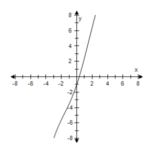
B)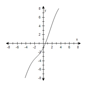
C)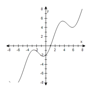
D)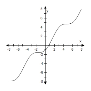
E)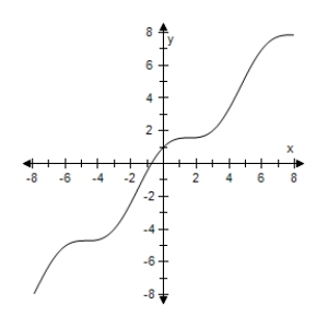
A)
B)
C)
D)
E)
سؤال
Select the graph of the function below.Include two full periods.
A)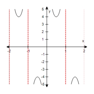
B)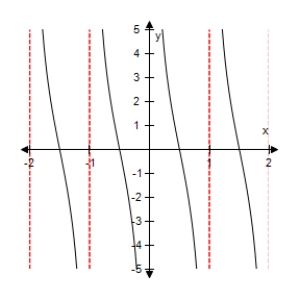
C)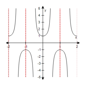
D)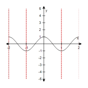
E)
A)
B)
C)
D)
E)
سؤال
Use a graphing utility to select the graph of the two equations in the same viewing window.Use the graphs to determine whether the expressions are equivalent.
A)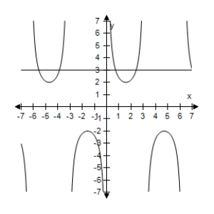 The expressions are equivalent except
Sinx = 0,y1 is undefined.
B) The expressions are equivalent except when sinx = 0,y1 is undefined.
C)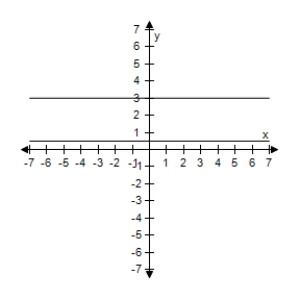 The expressions are equivalent except when
Sinx = 0,y1 is undefined.
D)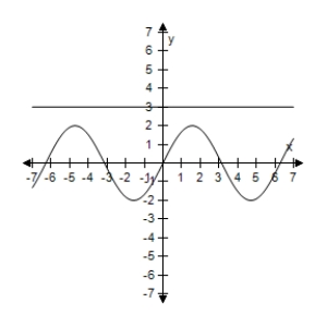 The expressions are equivalent except when sinx = 0,y1 is undefined.
E) The expressions are equivalent except when sinx = 0,y1 is undefined.
A)
The expressions are equivalent exceptSinx = 0,y1 is undefined.
B)
The expressions are equivalent except when sinx = 0,y1 is undefined.C)
The expressions are equivalent except whenSinx = 0,y1 is undefined.
D)
The expressions are equivalent except when sinx = 0,y1 is undefined.E)
The expressions are equivalent except when sinx = 0,y1 is undefined. سؤال
سؤال
سؤال
A plane flying at an altitude of a miles above a radar antenna will pass directly over the radar antenna (see figure).Let d be the ground distance from the antenna to the point directly under the plane and let x be the angle of elevation to the plane from the antenna. .
(d is positive as the plane approaches the antenna. )
Write d as a function of x.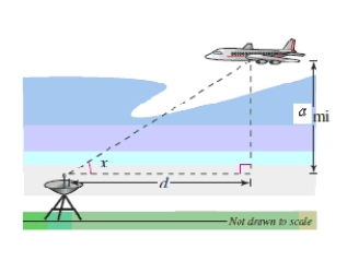
A)d = 8 csc x
B)d = 8 cot x
C)d = 8 cos x
D)d = 8 tan x
E)d = 8 sin x
(d is positive as the plane approaches the antenna. )
Write d as a function of x.
A)d = 8 csc x
B)d = 8 cot x
C)d = 8 cos x
D)d = 8 tan x
E)d = 8 sin x
سؤال
Select the graph of the function below.Include two full periods.
A)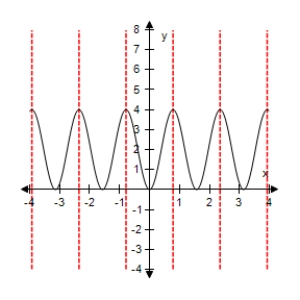
B)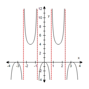
C)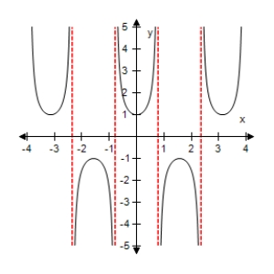
D)
E)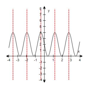
A)
B)
C)
D)
E)
سؤال
سؤال
سؤال
Select the graph of the function below.Include two full periods.
A)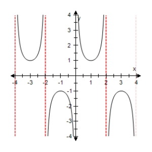
B)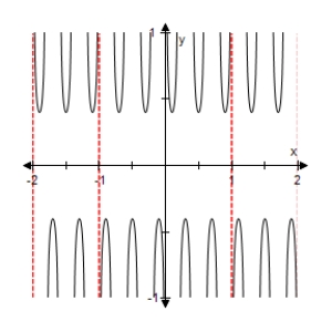
C)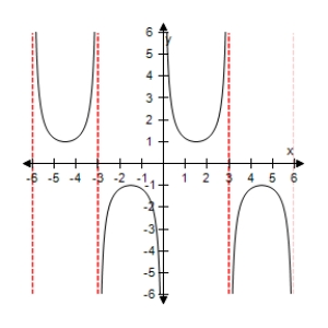
D)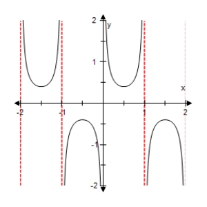
E)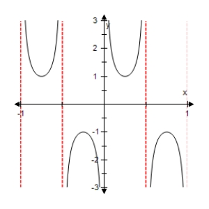
A)
B)
C)
D)
E)
سؤال
سؤال
سؤال
سؤال
Select the graph of the function below.Include two full periods.
A)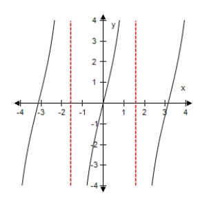
B)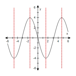
C)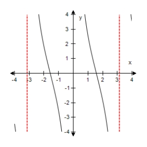
D)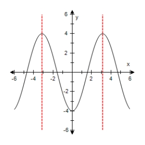
E)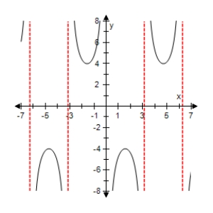
A)
B)
C)
D)
E)
سؤال
سؤال
Use a graphing utility to select the graph of the function:
A)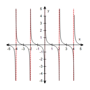
B)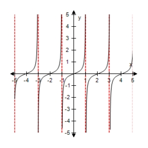
C)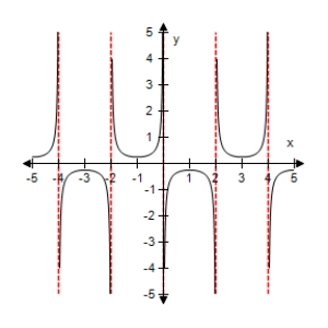
D)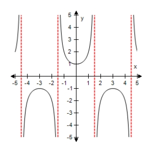
E)
A)
B)
C)
D)
E)
سؤال
Select the graph of the function below.Include two full periods.
A)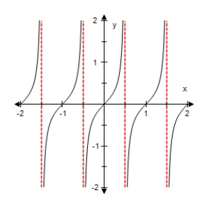
B)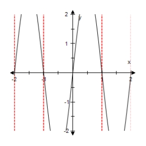
C)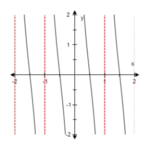
D)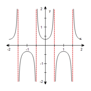
E)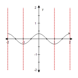
A)
B)
C)
D)
E)
سؤال
Use a graphing utility to select the graph of the function:
A)
B)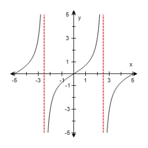
C)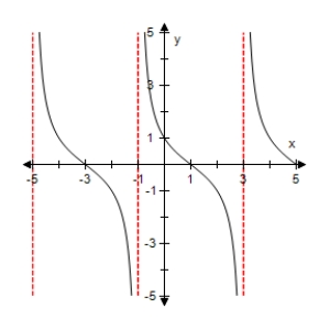
D)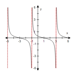
E)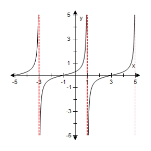
A)
B)
C)
D)
E)
سؤال
Select the graph of the function below.Include two full periods.
A)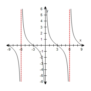
B)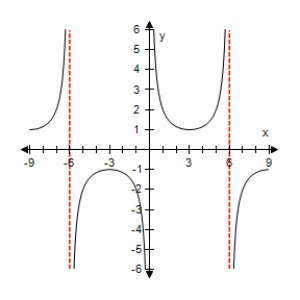
C)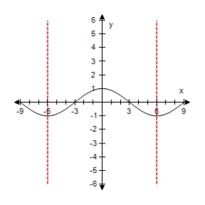
D)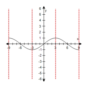
E)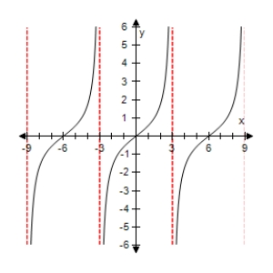
A)
B)
C)
D)
E)
سؤال
Use a graphing utility to select the graph of the function below and the damping factor of the function in the same viewing window.
A)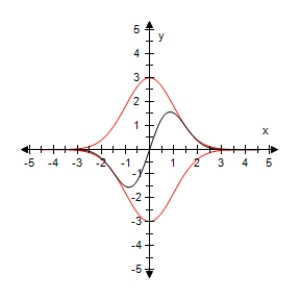
B)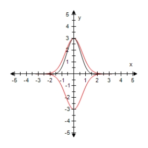
C)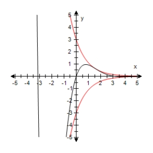
D)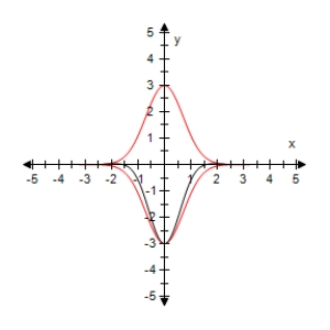
E)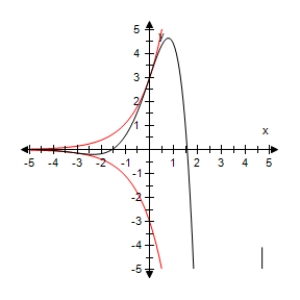
A)
B)
C)
D)
E)
سؤال
سؤال
سؤال
Use a graphing utility to select the graph of the function below and the damping factor of the function in the same viewing window.
A)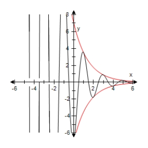
B)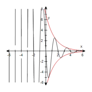
C)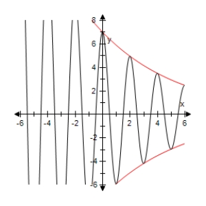
D)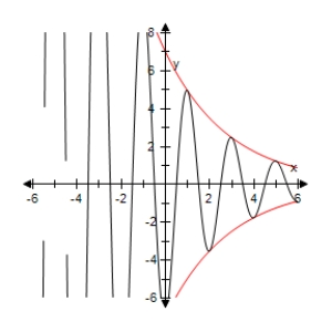
E)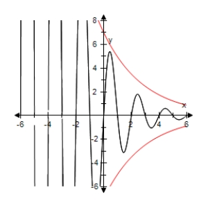
A)
B)
C)
D)
E)
سؤال
The projected monthly sales (in thousands of units)of lawn mowers (a seasonal product)are modeled by where t is the time (in months),with t = 1 corresponding to January.Select the graph of the sales function over 1 year.
A)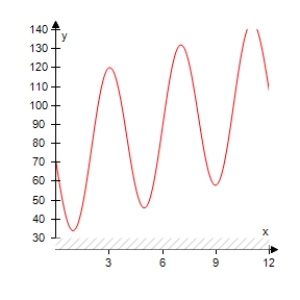
B)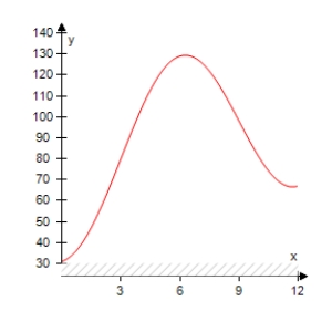
C)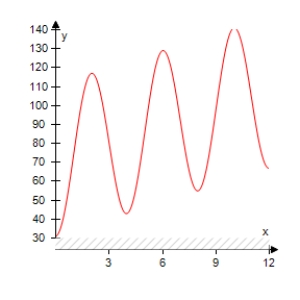
D)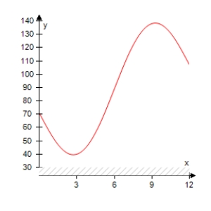
E)
A)
B)
C)
D)
E)
سؤال
سؤال
Use a graphing utility to select the graph of the function
A)
B)
C)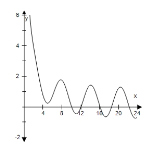
D)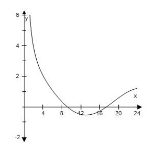
E)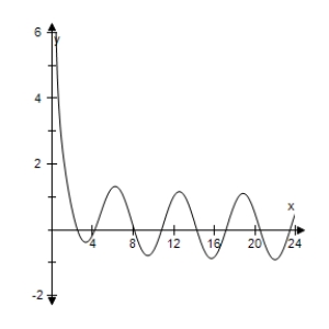
A)
B)
C)
D)
E)
سؤال
سؤال
سؤال
سؤال
Use a graphing utility to select the graph of the function below and the damping factor of the function in the same viewing window.
A)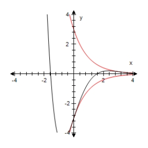
B)
C)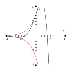
D)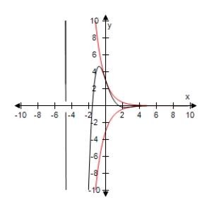
E)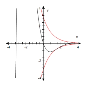
A)
B)
C)
D)
E)
سؤال
سؤال
A television camera is on a reviewing platform a meters from the street on which a parade will be passing from left to right (see figure).Write the distance d from the camera to a particular unit in the parade as a function of the angle x. a = 26. 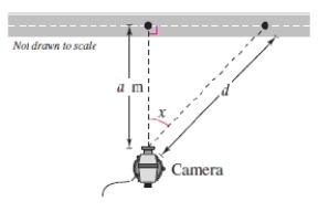
A)d = 26tan x
B)d = 26sec x
C)d = 26cos x
D)d = 26cot x
E)d = 26sin x
A)d = 26tan x
B)d = 26sec x
C)d = 26cos x
D)d = 26cot x
E)d = 26sin x
سؤال
سؤال
سؤال
سؤال
سؤال
سؤال
سؤال
سؤال
Use a graphing utility to select the graph the damping factor and the function below in the same viewing window.Describe the behavior of the function as x increases without bound.
A)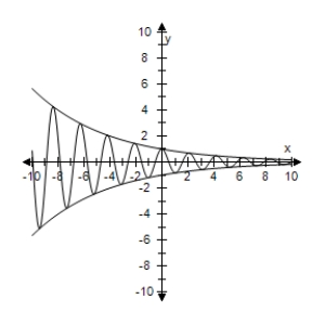 As x → ∞,f(x)→ 0.
B)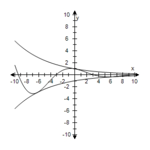 As x → ∞,f(x)→ 0.
C)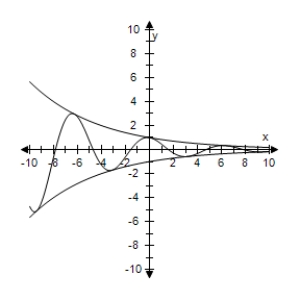 As x → ∞,f(x)→ 0.
D)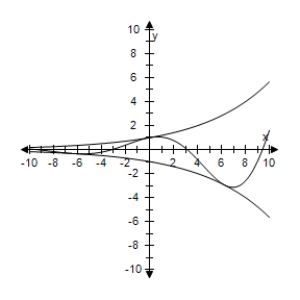 The function f(x)is unbounded as x → ∞.
E)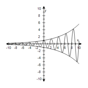 The function f(x)is unbounded as x → ∞.
A)
As x → ∞,f(x)→ 0.B)
As x → ∞,f(x)→ 0.C)
As x → ∞,f(x)→ 0.D)
The function f(x)is unbounded as x → ∞.E)
The function f(x)is unbounded as x → ∞. سؤال
Select the graph of the given function.Make sure to include at least two periods.
A)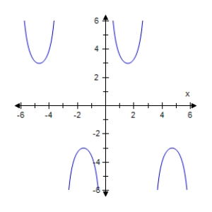
B)
C)
D)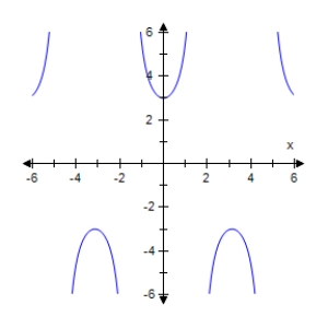
E)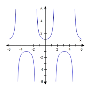
A)
B)
C)
D)
E)
سؤال
Use a graphing utility to select the graph the damping factor and the function below in the same viewing window.Describe the behavior of the function as x increases without bound.
A)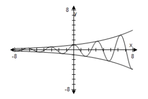 As x → ∞,f(x)→ ∞.
B)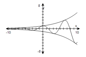 As x → ∞,f(x)→ ∞.
C)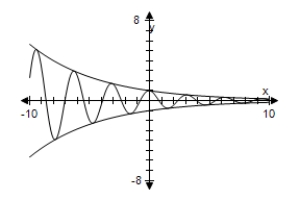 As x → ∞,f(x)→ 0.
D)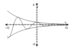 As x → ∞,f(x)→ 0.
E)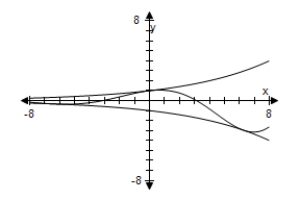 As x → ∞,f(x)→ ∞.
A)
As x → ∞,f(x)→ ∞.B)
As x → ∞,f(x)→ ∞.C)
As x → ∞,f(x)→ 0.D)
As x → ∞,f(x)→ 0.E)
As x → ∞,f(x)→ ∞. سؤال
Select the graph of the given function.Make sure to include at least two periods.
A)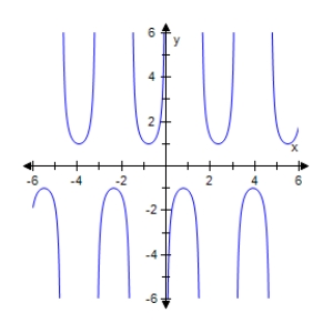
B)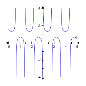
C)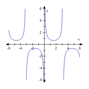
D)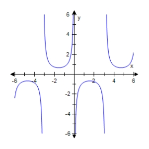
E)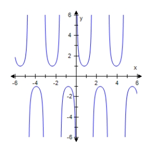
A)
B)
C)
D)
E)
سؤال
Use a graphing utility to select the graph of the function below,making sure to show at least two periods. 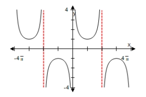
Xscl = 
Xscl =
Xscl =
Xscl =
A)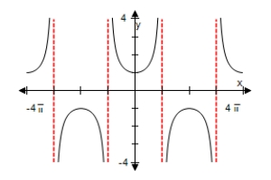
B)
C) 
D) 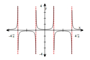
E) 
Xscl =
Xscl =
Xscl =
Xscl =
A)
B)
C)
D)
E)
سؤال
Use a graphing utility to select the graph of the expression below,making sure to show at least two periods.
A)
B)
C)
D)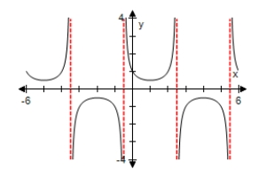
E)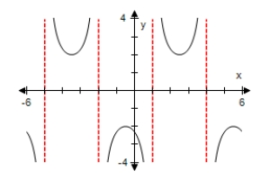
A)
B)
C)
D)
E)
سؤال
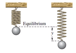
An object weighing W pounds is suspended from the ceiling by a steel spring (see figure).The weight is pulled downward (positive direction)from its equilibrium position and released.The resulting motion of the weight is described by the function where y is the distance (in feet)and t is the time (in seconds).
Use a graphing utility to select the graph of the function.
A)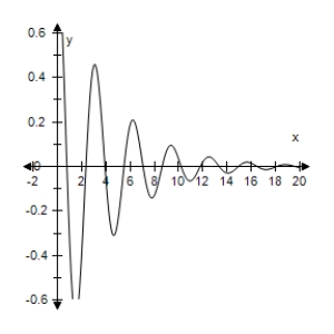
B)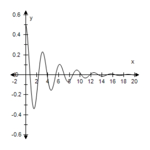
C)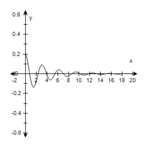
D)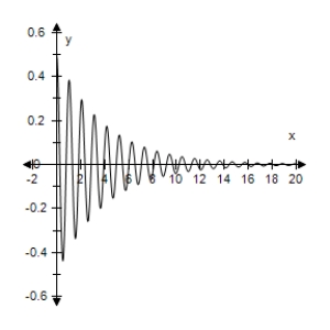
E)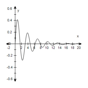
Use a graphing utility to select the graph of the function.
A)
B)
C)
D)
E)
سؤال
Use the graph shown below to determine if the function is even,odd,or neither. 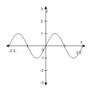
A)Even
B)Odd
C)Neither
A)Even
B)Odd
C)Neither
سؤال
Determine which of the graphs below represents
A)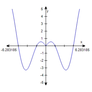
B)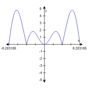
C)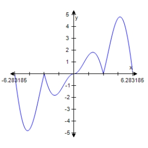
D)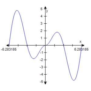
E)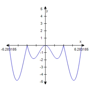
A)
B)
C)
D)
E)
سؤال
Use a graphing utility to select the graph of the function below.Describe the behavior of the function as x approaches 0.
A)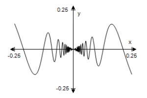 As x → 0,f(x)→ 0.
B)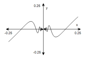 As x → 0,f(x)→ 0.
C)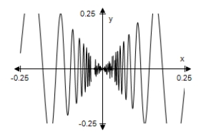 As x → 0,f(x)→ 0.
D)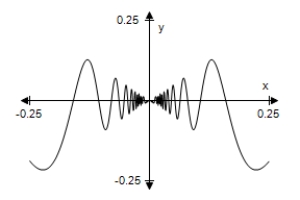 As x → 0,f(x)→ 0.
E)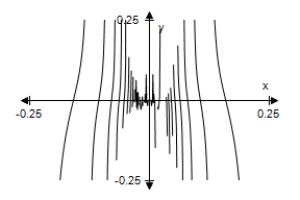 As x → 0,f(x)→ 0.
A)
As x → 0,f(x)→ 0.B)
As x → 0,f(x)→ 0.C)
As x → 0,f(x)→ 0.D)
As x → 0,f(x)→ 0.E)
As x → 0,f(x)→ 0. سؤال
Which of the following functions is represented by the graph below? 
A)
B)
C)
D)
E)
A)
B)
C)
D)
E)

فتح الحزمة
قم بالتسجيل لفتح البطاقات في هذه المجموعة!
Unlock Deck
Unlock Deck
1/51
العب
ملء الشاشة (f)
Deck 28: Graphs of Other Trigonometric Functions
1
Determine whether the function below is even,odd,or neither.
A)Even
B)Odd
C)Neither
A)Even
B)Odd
C)Neither
Odd
2
Consider the function given by Use a graphing utility to select the graph of the function.
A)
B)
C)
D)
E)
A)
B)
C)
D)
E)
3
Select the graph of the function below.Include two full periods.
A)
B)
C)
D)
E)
A)
B)
C)
D)
E)
4
Use a graphing utility to select the graph of the two equations in the same viewing window.Use the graphs to determine whether the expressions are equivalent.
A) The expressions are equivalent except
Sinx = 0,y1 is undefined.
B) The expressions are equivalent except when sinx = 0,y1 is undefined.
C) The expressions are equivalent except when
Sinx = 0,y1 is undefined.
D) The expressions are equivalent except when sinx = 0,y1 is undefined.
E) The expressions are equivalent except when sinx = 0,y1 is undefined.
A)
The expressions are equivalent exceptSinx = 0,y1 is undefined.
B)
The expressions are equivalent except when sinx = 0,y1 is undefined.C)
The expressions are equivalent except whenSinx = 0,y1 is undefined.
D)
The expressions are equivalent except when sinx = 0,y1 is undefined.E)
The expressions are equivalent except when sinx = 0,y1 is undefined. فتح الحزمة
افتح القفل للوصول البطاقات البالغ عددها 51 في هذه المجموعة.
فتح الحزمة
k this deck
5
State the period of the function:
A)
B)
C)
D)
E)1
A)
B)
C)
D)
E)1
فتح الحزمة
افتح القفل للوصول البطاقات البالغ عددها 51 في هذه المجموعة.
فتح الحزمة
k this deck
6
Determine whether the function below is even,odd,or neither.
A)Neither
B)Odd
C)Even
A)Neither
B)Odd
C)Even
فتح الحزمة
افتح القفل للوصول البطاقات البالغ عددها 51 في هذه المجموعة.
فتح الحزمة
k this deck
7
A plane flying at an altitude of a miles above a radar antenna will pass directly over the radar antenna (see figure).Let d be the ground distance from the antenna to the point directly under the plane and let x be the angle of elevation to the plane from the antenna. .
(d is positive as the plane approaches the antenna. )
Write d as a function of x.
A)d = 8 csc x
B)d = 8 cot x
C)d = 8 cos x
D)d = 8 tan x
E)d = 8 sin x
(d is positive as the plane approaches the antenna. )
Write d as a function of x.
A)d = 8 csc x
B)d = 8 cot x
C)d = 8 cos x
D)d = 8 tan x
E)d = 8 sin x
فتح الحزمة
افتح القفل للوصول البطاقات البالغ عددها 51 في هذه المجموعة.
فتح الحزمة
k this deck
8
Select the graph of the function below.Include two full periods.
A)
B)
C)
D)
E)
A)
B)
C)
D)
E)
فتح الحزمة
افتح القفل للوصول البطاقات البالغ عددها 51 في هذه المجموعة.
فتح الحزمة
k this deck
9
State the period of the function:
A)14
B)10
C)
D)
E)12
A)14
B)10
C)
D)
E)12
فتح الحزمة
افتح القفل للوصول البطاقات البالغ عددها 51 في هذه المجموعة.
فتح الحزمة
k this deck
10
State the period of the function:
A)
B)
C)
D)
E)
A)
B)
C)
D)
E)
فتح الحزمة
افتح القفل للوصول البطاقات البالغ عددها 51 في هذه المجموعة.
فتح الحزمة
k this deck
11
Select the graph of the function below.Include two full periods.
A)
B)
C)
D)
E)
A)
B)
C)
D)
E)
فتح الحزمة
افتح القفل للوصول البطاقات البالغ عددها 51 في هذه المجموعة.
فتح الحزمة
k this deck
12
Consider the functions given by
on the interval (0,π). Describe the behavior of each of the functions as x approaches π.
A)f approaches 2 and g approaches +∞.
B)f approaches 0 and g approaches +∞.
C)f approaches +∞ and g approaches 0.
D)f approaches 0 and g approaches .
E)f approaches 2 and g approaches .
on the interval (0,π). Describe the behavior of each of the functions as x approaches π.
A)f approaches 2 and g approaches +∞.
B)f approaches 0 and g approaches +∞.
C)f approaches +∞ and g approaches 0.
D)f approaches 0 and g approaches .
E)f approaches 2 and g approaches .
فتح الحزمة
افتح القفل للوصول البطاقات البالغ عددها 51 في هذه المجموعة.
فتح الحزمة
k this deck
13
State the period of the function:
A)
B)6
C)8
D)
E)12
A)
B)6
C)8
D)
E)12
فتح الحزمة
افتح القفل للوصول البطاقات البالغ عددها 51 في هذه المجموعة.
فتح الحزمة
k this deck
14
State the period of the function:
A)
B)
C)
D)
E)
A)
B)
C)
D)
E)
فتح الحزمة
افتح القفل للوصول البطاقات البالغ عددها 51 في هذه المجموعة.
فتح الحزمة
k this deck
15
Select the graph of the function below.Include two full periods.
A)
B)
C)
D)
E)
A)
B)
C)
D)
E)
فتح الحزمة
افتح القفل للوصول البطاقات البالغ عددها 51 في هذه المجموعة.
فتح الحزمة
k this deck
16
State the period of the function:
A)
B)
C)
D)
E)
A)
B)
C)
D)
E)
فتح الحزمة
افتح القفل للوصول البطاقات البالغ عددها 51 في هذه المجموعة.
فتح الحزمة
k this deck
17
Use a graphing utility to select the graph of the function:
A)
B)
C)
D)
E)
A)
B)
C)
D)
E)
فتح الحزمة
افتح القفل للوصول البطاقات البالغ عددها 51 في هذه المجموعة.
فتح الحزمة
k this deck
18
Select the graph of the function below.Include two full periods.
A)
B)
C)
D)
E)
A)
B)
C)
D)
E)
فتح الحزمة
افتح القفل للوصول البطاقات البالغ عددها 51 في هذه المجموعة.
فتح الحزمة
k this deck
19
Use a graphing utility to select the graph of the function:
A)
B)
C)
D)
E)
A)
B)
C)
D)
E)
فتح الحزمة
افتح القفل للوصول البطاقات البالغ عددها 51 في هذه المجموعة.
فتح الحزمة
k this deck
20
Select the graph of the function below.Include two full periods.
A)
B)
C)
D)
E)
A)
B)
C)
D)
E)
فتح الحزمة
افتح القفل للوصول البطاقات البالغ عددها 51 في هذه المجموعة.
فتح الحزمة
k this deck
21
Use a graphing utility to select the graph of the function below and the damping factor of the function in the same viewing window.
A)
B)
C)
D)
E)
A)
B)
C)
D)
E)
فتح الحزمة
افتح القفل للوصول البطاقات البالغ عددها 51 في هذه المجموعة.
فتح الحزمة
k this deck
22
Describe the behavior of the function below as x approaches .
A)f → +∞ as x → .
B)f → 0 as x → .
C)f → -∞ as x → .
D)f → 1 as x → .
E)f → -1 as x → .
A)f → +∞ as x → .
B)f → 0 as x → .
C)f → -∞ as x → .
D)f → 1 as x → .
E)f → -1 as x → .
فتح الحزمة
افتح القفل للوصول البطاقات البالغ عددها 51 في هذه المجموعة.
فتح الحزمة
k this deck
23
Describe the behavior of the function below as x approaches zero.
A)f → -∞ as x → 0.
B)f → -1 as x → 0.
C)f → 1 as x → 0.
D)f → +∞ as x → 0.
E)f → 0 as x → 0.
A)f → -∞ as x → 0.
B)f → -1 as x → 0.
C)f → 1 as x → 0.
D)f → +∞ as x → 0.
E)f → 0 as x → 0.
فتح الحزمة
افتح القفل للوصول البطاقات البالغ عددها 51 في هذه المجموعة.
فتح الحزمة
k this deck
24
Use a graphing utility to select the graph of the function below and the damping factor of the function in the same viewing window.
A)
B)
C)
D)
E)
A)
B)
C)
D)
E)
فتح الحزمة
افتح القفل للوصول البطاقات البالغ عددها 51 في هذه المجموعة.
فتح الحزمة
k this deck
25
The projected monthly sales (in thousands of units)of lawn mowers (a seasonal product)are modeled by where t is the time (in months),with t = 1 corresponding to January.Select the graph of the sales function over 1 year.
A)
B)
C)
D)
E)
A)
B)
C)
D)
E)
فتح الحزمة
افتح القفل للوصول البطاقات البالغ عددها 51 في هذه المجموعة.
فتح الحزمة
k this deck
26
Describe the behavior of the function below as x approaches zero.
A)f → 0 as x → 0.
B)f → -1 as x → 0.
C)f → 1 as x → 0.
D)f → -∞ as x → 0.
E)f → +∞ as x → 0.
A)f → 0 as x → 0.
B)f → -1 as x → 0.
C)f → 1 as x → 0.
D)f → -∞ as x → 0.
E)f → +∞ as x → 0.
فتح الحزمة
افتح القفل للوصول البطاقات البالغ عددها 51 في هذه المجموعة.
فتح الحزمة
k this deck
27
Use a graphing utility to select the graph of the function
A)
B)
C)
D)
E)
A)
B)
C)
D)
E)
فتح الحزمة
افتح القفل للوصول البطاقات البالغ عددها 51 في هذه المجموعة.
فتح الحزمة
k this deck
28
Determine whether the function below is even,odd,or neither.
A)Neither
B)Even
C)Odd
A)Neither
B)Even
C)Odd
فتح الحزمة
افتح القفل للوصول البطاقات البالغ عددها 51 في هذه المجموعة.
فتح الحزمة
k this deck
29
Describe the behavior of the function below as x approaches π-.
A)f → -∞ as x → π-.
B)f → +∞ as x → π-.
C)f → 1 as x → π-.
D)f → 0 as x → π-.
E)f → -1 as x → π-.
A)f → -∞ as x → π-.
B)f → +∞ as x → π-.
C)f → 1 as x → π-.
D)f → 0 as x → π-.
E)f → -1 as x → π-.
فتح الحزمة
افتح القفل للوصول البطاقات البالغ عددها 51 في هذه المجموعة.
فتح الحزمة
k this deck
30
Determine whether the function below is even,odd,or neither.
A)Even
B)Odd
C)Neither
A)Even
B)Odd
C)Neither
فتح الحزمة
افتح القفل للوصول البطاقات البالغ عددها 51 في هذه المجموعة.
فتح الحزمة
k this deck
31
Use a graphing utility to select the graph of the function below and the damping factor of the function in the same viewing window.
A)
B)
C)
D)
E)
A)
B)
C)
D)
E)
فتح الحزمة
افتح القفل للوصول البطاقات البالغ عددها 51 في هذه المجموعة.
فتح الحزمة
k this deck
32
Describe the behavior of the function below as x approaches zero.
A)f → +∞ as x → 0.
B)f → 1 as x → 0.
C)f → 0 as x → 0.
D)f → -1 as x → 0.
E)f → -∞ as x → 0.
A)f → +∞ as x → 0.
B)f → 1 as x → 0.
C)f → 0 as x → 0.
D)f → -1 as x → 0.
E)f → -∞ as x → 0.
فتح الحزمة
افتح القفل للوصول البطاقات البالغ عددها 51 في هذه المجموعة.
فتح الحزمة
k this deck
33
A television camera is on a reviewing platform a meters from the street on which a parade will be passing from left to right (see figure).Write the distance d from the camera to a particular unit in the parade as a function of the angle x. a = 26.
A)d = 26tan x
B)d = 26sec x
C)d = 26cos x
D)d = 26cot x
E)d = 26sin x
A)d = 26tan x
B)d = 26sec x
C)d = 26cos x
D)d = 26cot x
E)d = 26sin x
فتح الحزمة
افتح القفل للوصول البطاقات البالغ عددها 51 في هذه المجموعة.
فتح الحزمة
k this deck
34
Describe the behavior of the function below as x approaches 0+.
A)f → +∞ as x → 0+.
B)f → 0 as x → 0+.
C)f → -1 as x → 0+.
D)f → -∞ as x → 0+.
E)f → 1 as x → 0+.
A)f → +∞ as x → 0+.
B)f → 0 as x → 0+.
C)f → -1 as x → 0+.
D)f → -∞ as x → 0+.
E)f → 1 as x → 0+.
فتح الحزمة
افتح القفل للوصول البطاقات البالغ عددها 51 في هذه المجموعة.
فتح الحزمة
k this deck
35
Describe the behavior of the function below as x approaches zero.
A)f → +∞ as x → 0.
B)f → 1 as x → 0.
C)f → 0 as x → 0.
D)f → -1 as x → 0.
E)f → -∞ as x → 0.
A)f → +∞ as x → 0.
B)f → 1 as x → 0.
C)f → 0 as x → 0.
D)f → -1 as x → 0.
E)f → -∞ as x → 0.
فتح الحزمة
افتح القفل للوصول البطاقات البالغ عددها 51 في هذه المجموعة.
فتح الحزمة
k this deck
36
Determine whether the function below is even,odd,or neither.
A)Neither
B)Odd
C)Even
A)Neither
B)Odd
C)Even
فتح الحزمة
افتح القفل للوصول البطاقات البالغ عددها 51 في هذه المجموعة.
فتح الحزمة
k this deck
37
Determine whether the function below is even,odd,or neither.
F(x)= 0.8 cot x
A)Neither
B)Even
C)Odd
F(x)= 0.8 cot x
A)Neither
B)Even
C)Odd
فتح الحزمة
افتح القفل للوصول البطاقات البالغ عددها 51 في هذه المجموعة.
فتح الحزمة
k this deck
38
Determine whether the function below is even,odd,or neither.
A)Even
B)Odd
C)Neither
A)Even
B)Odd
C)Neither
فتح الحزمة
افتح القفل للوصول البطاقات البالغ عددها 51 في هذه المجموعة.
فتح الحزمة
k this deck
39
Describe the behavior of the function below as x approaches .
A)f → +∞ as x → .
B)f → 0 as x → .
C)f → 1 as x → .
D)f → -∞ as x → .
E)f → -1 as x → .
A)f → +∞ as x → .
B)f → 0 as x → .
C)f → 1 as x → .
D)f → -∞ as x → .
E)f → -1 as x → .
فتح الحزمة
افتح القفل للوصول البطاقات البالغ عددها 51 في هذه المجموعة.
فتح الحزمة
k this deck
40
Determine whether the function below is even,odd,or neither.
A)Neither
B)Odd
C)Even
A)Neither
B)Odd
C)Even
فتح الحزمة
افتح القفل للوصول البطاقات البالغ عددها 51 في هذه المجموعة.
فتح الحزمة
k this deck
41
Use a graphing utility to select the graph the damping factor and the function below in the same viewing window.Describe the behavior of the function as x increases without bound.
A) As x → ∞,f(x)→ 0.
B) As x → ∞,f(x)→ 0.
C) As x → ∞,f(x)→ 0.
D) The function f(x)is unbounded as x → ∞.
E) The function f(x)is unbounded as x → ∞.
A)
As x → ∞,f(x)→ 0.B)
As x → ∞,f(x)→ 0.C)
As x → ∞,f(x)→ 0.D)
The function f(x)is unbounded as x → ∞.E)
The function f(x)is unbounded as x → ∞. فتح الحزمة
افتح القفل للوصول البطاقات البالغ عددها 51 في هذه المجموعة.
فتح الحزمة
k this deck
42
Select the graph of the given function.Make sure to include at least two periods.
A)
B)
C)
D)
E)
A)
B)
C)
D)
E)
فتح الحزمة
افتح القفل للوصول البطاقات البالغ عددها 51 في هذه المجموعة.
فتح الحزمة
k this deck
43
Use a graphing utility to select the graph the damping factor and the function below in the same viewing window.Describe the behavior of the function as x increases without bound.
A) As x → ∞,f(x)→ ∞.
B) As x → ∞,f(x)→ ∞.
C) As x → ∞,f(x)→ 0.
D) As x → ∞,f(x)→ 0.
E) As x → ∞,f(x)→ ∞.
A)
As x → ∞,f(x)→ ∞.B)
As x → ∞,f(x)→ ∞.C)
As x → ∞,f(x)→ 0.D)
As x → ∞,f(x)→ 0.E)
As x → ∞,f(x)→ ∞. فتح الحزمة
افتح القفل للوصول البطاقات البالغ عددها 51 في هذه المجموعة.
فتح الحزمة
k this deck
44
Select the graph of the given function.Make sure to include at least two periods.
A)
B)
C)
D)
E)
A)
B)
C)
D)
E)
فتح الحزمة
افتح القفل للوصول البطاقات البالغ عددها 51 في هذه المجموعة.
فتح الحزمة
k this deck
45
Use a graphing utility to select the graph of the function below,making sure to show at least two periods.
Xscl =
Xscl =
Xscl =
Xscl =
A)
B)
C)
D)
E)
Xscl =
Xscl =
Xscl =
Xscl =
A)
B)
C)
D)
E)
فتح الحزمة
افتح القفل للوصول البطاقات البالغ عددها 51 في هذه المجموعة.
فتح الحزمة
k this deck
46
Use a graphing utility to select the graph of the expression below,making sure to show at least two periods.
A)
B)
C)
D)
E)
A)
B)
C)
D)
E)
فتح الحزمة
افتح القفل للوصول البطاقات البالغ عددها 51 في هذه المجموعة.
فتح الحزمة
k this deck
47
An object weighing W pounds is suspended from the ceiling by a steel spring (see figure).The weight is pulled downward (positive direction)from its equilibrium position and released.The resulting motion of the weight is described by the function where y is the distance (in feet)and t is the time (in seconds).
Use a graphing utility to select the graph of the function.
A)
B)
C)
D)
E)
Use a graphing utility to select the graph of the function.
A)
B)
C)
D)
E)
فتح الحزمة
افتح القفل للوصول البطاقات البالغ عددها 51 في هذه المجموعة.
فتح الحزمة
k this deck
48
Use the graph shown below to determine if the function is even,odd,or neither.
A)Even
B)Odd
C)Neither
A)Even
B)Odd
C)Neither
فتح الحزمة
افتح القفل للوصول البطاقات البالغ عددها 51 في هذه المجموعة.
فتح الحزمة
k this deck
49
Determine which of the graphs below represents
A)
B)
C)
D)
E)
A)
B)
C)
D)
E)
فتح الحزمة
افتح القفل للوصول البطاقات البالغ عددها 51 في هذه المجموعة.
فتح الحزمة
k this deck
50
Use a graphing utility to select the graph of the function below.Describe the behavior of the function as x approaches 0.
A) As x → 0,f(x)→ 0.
B) As x → 0,f(x)→ 0.
C) As x → 0,f(x)→ 0.
D) As x → 0,f(x)→ 0.
E) As x → 0,f(x)→ 0.
A)
As x → 0,f(x)→ 0.B)
As x → 0,f(x)→ 0.C)
As x → 0,f(x)→ 0.D)
As x → 0,f(x)→ 0.E)
As x → 0,f(x)→ 0. فتح الحزمة
افتح القفل للوصول البطاقات البالغ عددها 51 في هذه المجموعة.
فتح الحزمة
k this deck
51
Which of the following functions is represented by the graph below?
A)
B)
C)
D)
E)
A)
B)
C)
D)
E)
فتح الحزمة
افتح القفل للوصول البطاقات البالغ عددها 51 في هذه المجموعة.
فتح الحزمة
k this deck
فتح الحزمة
افتح القفل للوصول البطاقات البالغ عددها 51 في هذه المجموعة.


