Deck 13: Analysis of Variance
ملء الشاشة (f)
سؤال
Fisher's 100(1 - α)% confidence interval for the difference between two population means μi - μj is:
A)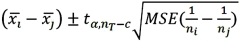
B)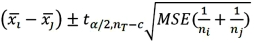
C)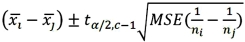
D)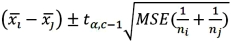
A)
B)
C)
D)
سؤال
سؤال
سؤال
سؤال
سؤال
سؤال
سؤال
سؤال
سؤال
سؤال
سؤال
سؤال
سؤال
سؤال
سؤال
سؤال
سؤال
سؤال
سؤال
سؤال
Exhibit 13.2 A researcher with Ministry of Transportation is commissioned to study the drive times to work (one-way)for U.S.cities.The underlying hypothesis is that average commute times are different across cities.To test the hypothesis,the researcher randomly selects six people from each of the four cities and records their one-way commute times to work.Refer to the below data on one-way commute time (in minutes)to work.Note that the grand mean is 36.625. 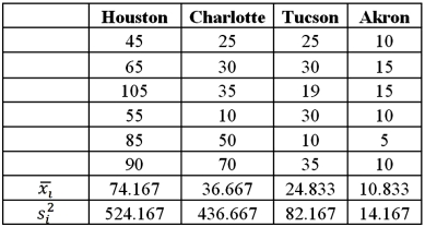 Refer to Exhibit 13.2.Which of the following is the sum of squared errors?
A)264.29
B)5,285.83
C)18,567.63
D)13,281.79
Refer to Exhibit 13.2.Which of the following is the sum of squared errors?A)264.29
B)5,285.83
C)18,567.63
D)13,281.79
سؤال
سؤال
Tukey's 100(1 - α)% confidence interval for the difference between two population means μi - μj for balanced data is given by ____.
A)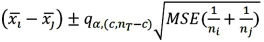
B)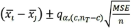
C)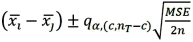
D)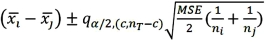
A)
B)
C)
D)
سؤال
Exhibit 13.2 A researcher with Ministry of Transportation is commissioned to study the drive times to work (one-way)for U.S.cities.The underlying hypothesis is that average commute times are different across cities.To test the hypothesis,the researcher randomly selects six people from each of the four cities and records their one-way commute times to work.Refer to the below data on one-way commute time (in minutes)to work.Note that the grand mean is 36.625.  Refer to Exhibit 13.2.At the 5% significance level,the critical value is:
A)2.38
B)3.10
C)3.86
D)4.94
Refer to Exhibit 13.2.At the 5% significance level,the critical value is:A)2.38
B)3.10
C)3.86
D)4.94
سؤال
سؤال
سؤال
سؤال
Exhibit 13.2 A researcher with Ministry of Transportation is commissioned to study the drive times to work (one-way)for U.S.cities.The underlying hypothesis is that average commute times are different across cities.To test the hypothesis,the researcher randomly selects six people from each of the four cities and records their one-way commute times to work.Refer to the below data on one-way commute time (in minutes)to work.Note that the grand mean is 36.625.  Refer to Exhibit 13.2.The conclusion for the hypothesis test is:
A)Reject the null hypothesis,cannot conclude that not all mean commute times are equal
B)Do not reject the null hypothesis,cannot conclude that not all mean commute times are equal
C)Reject the null hypothesis,not all mean commute times are equal
D)Do not reject the null hypothesis,not all mean commute times are equal
Refer to Exhibit 13.2.The conclusion for the hypothesis test is:A)Reject the null hypothesis,cannot conclude that not all mean commute times are equal
B)Do not reject the null hypothesis,cannot conclude that not all mean commute times are equal
C)Reject the null hypothesis,not all mean commute times are equal
D)Do not reject the null hypothesis,not all mean commute times are equal
سؤال
Exhibit 13.2 A researcher with Ministry of Transportation is commissioned to study the drive times to work (one-way)for U.S.cities.The underlying hypothesis is that average commute times are different across cities.To test the hypothesis,the researcher randomly selects six people from each of the four cities and records their one-way commute times to work.Refer to the below data on one-way commute time (in minutes)to work.Note that the grand mean is 36.625.  Refer to Exhibit 13.2.Which of the following is the sum of squares due to treatments?
A)5,285.83
B)13,281.79
C)18,567.63
D)4,427.26
Refer to Exhibit 13.2.Which of the following is the sum of squares due to treatments?A)5,285.83
B)13,281.79
C)18,567.63
D)4,427.26
سؤال
Exhibit 13.2 A researcher with Ministry of Transportation is commissioned to study the drive times to work (one-way)for U.S.cities.The underlying hypothesis is that average commute times are different across cities.To test the hypothesis,the researcher randomly selects six people from each of the four cities and records their one-way commute times to work.Refer to the below data on one-way commute time (in minutes)to work.Note that the grand mean is 36.625. 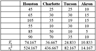 Refer to Exhibit 13.2.The value of the test statistic is:
A)0.06
B)0.40
C)2.51
D)16.75
Refer to Exhibit 13.2.The value of the test statistic is:A)0.06
B)0.40
C)2.51
D)16.75
سؤال
Exhibit 13.2 A researcher with Ministry of Transportation is commissioned to study the drive times to work (one-way)for U.S.cities.The underlying hypothesis is that average commute times are different across cities.To test the hypothesis,the researcher randomly selects six people from each of the four cities and records their one-way commute times to work.Refer to the below data on one-way commute time (in minutes)to work.Note that the grand mean is 36.625.  Refer to Exhibit 13.2.Based on the sample standard deviation,the one-way ANOVA assumption which is likely not met is:
A)The populations are normally distributed
B)The population standard deviations are assumed to be equal
C)The samples are independent
D)None of the above
Refer to Exhibit 13.2.Based on the sample standard deviation,the one-way ANOVA assumption which is likely not met is:A)The populations are normally distributed
B)The population standard deviations are assumed to be equal
C)The samples are independent
D)None of the above
سؤال
Exhibit 13.2 A researcher with Ministry of Transportation is commissioned to study the drive times to work (one-way)for U.S.cities.The underlying hypothesis is that average commute times are different across cities.To test the hypothesis,the researcher randomly selects six people from each of the four cities and records their one-way commute times to work.Refer to the below data on one-way commute time (in minutes)to work.Note that the grand mean is 36.625.  Refer to Exhibit 13.2.The competing hypotheses about the mean commute times are:
A)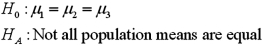
B)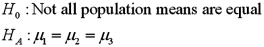
C)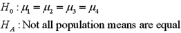
D)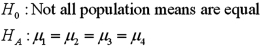
Refer to Exhibit 13.2.The competing hypotheses about the mean commute times are:A)
B)
C)
D)
سؤال
Exhibit 13.1 The following is an incomplete ANOVA table.  Refer to Exhibit 13.1.The value of the test statistic is:
A)1.333
B)9.375
C)12.5
D)100
Refer to Exhibit 13.1.The value of the test statistic is:A)1.333
B)9.375
C)12.5
D)100
سؤال
سؤال
سؤال
Exhibit 13.1 The following is an incomplete ANOVA table.  Refer to Exhibit 13.1.The mean square error is:
A)1.333
B)9.375
C)25
D)75
Refer to Exhibit 13.1.The mean square error is:A)1.333
B)9.375
C)25
D)75
سؤال
Exhibit 13.2 A researcher with Ministry of Transportation is commissioned to study the drive times to work (one-way)for U.S.cities.The underlying hypothesis is that average commute times are different across cities.To test the hypothesis,the researcher randomly selects six people from each of the four cities and records their one-way commute times to work.Refer to the below data on one-way commute time (in minutes)to work.Note that the grand mean is 36.625.  Refer to Exhibit 13.2.Which of the following is the mean square for treatments?
A)18,567.63
B)13,281.79
C)5,285.83
D)4,427.26
Refer to Exhibit 13.2.Which of the following is the mean square for treatments?A)18,567.63
B)13,281.79
C)5,285.83
D)4,427.26
سؤال
Exhibit 13.1 The following is an incomplete ANOVA table.  Refer to exhibit 13.1.The sum of squares due to treatments is:
A)10
B)25
C)75
D)100
Refer to exhibit 13.1.The sum of squares due to treatments is:A)10
B)25
C)75
D)100
سؤال
Exhibit 13.1 The following is an incomplete ANOVA table.  Refer to Exhibit 13.1.For the within groups,the degrees of freedom are:
A)6
B)7
C)8
D)9
Refer to Exhibit 13.1.For the within groups,the degrees of freedom are:A)6
B)7
C)8
D)9
سؤال
Exhibit 13.1 The following is an incomplete ANOVA table. 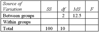 Refer to Exhibit 13.1.At the 5% significance level,the critical value is:
A)3.11
B)4.46
C)6.06
D)8.65
Refer to Exhibit 13.1.At the 5% significance level,the critical value is:A)3.11
B)4.46
C)6.06
D)8.65
سؤال
Exhibit 13.4 The ANOVA test performed for Exhibit 13.2 determined that not all mean commute times across the four cities are equal.However,it did not indicate which means differed.To find out which population means differ requires further analysis of the direction and the statistical significance of the difference between paired population means.Tukey 95% confidence intervals are shown below. 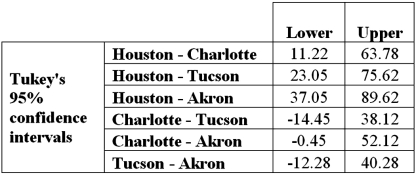 Refer to Exhibit 13.4.How many pairs of cities show a significant difference in average commute times to work?
A)2
B)3
C)4
D)6
Refer to Exhibit 13.4.How many pairs of cities show a significant difference in average commute times to work?A)2
B)3
C)4
D)6
سؤال
Exhibit 13.3 The ANOVA test performed for Exhibit 13.2 determined that not all mean commute times across the four cities are equal.However,it did not indicate which means differed.To find out which population means differ requires further analysis of the direction and the statistical significance of the difference between paired population means.Fisher 95% confidence intervals are shown below.  Refer to Exhibit 13.3.How many pairs of cities show a significant difference in average commute times to work?
A)2
B)3
C)4
D)6
Refer to Exhibit 13.3.How many pairs of cities show a significant difference in average commute times to work?A)2
B)3
C)4
D)6
سؤال
Exhibit 13.6 A researcher wants to understand how annual mortgage payment (in dollars)depends on income level and zonal location using a two-way ANOVA without interaction.The data and an incomplete ANOVA table are shown below. 
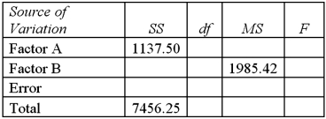 Refer to Exhibit 13.6.How many degrees of freedom are there for factors A and B?
A)2,3
B)3,4
C)3,6
D)2,4
Refer to Exhibit 13.6.How many degrees of freedom are there for factors A and B?A)2,3
B)3,4
C)3,6
D)2,4
سؤال
Exhibit 13.6 A researcher wants to understand how annual mortgage payment (in dollars)depends on income level and zonal location using a two-way ANOVA without interaction.The data and an incomplete ANOVA table are shown below. 
 Refer to Exhibit 13.6.At the 5% significance level,the conclusion for the hypothesis test about factor A is:
A)Do not reject the null hypothesis,the average mortgage payments differ by income level
B)Do not reject the null hypothesis,cannot conclude the average mortgage payments differ by income level
C)Reject the null hypothesis,the average mortgage payments differ by income level
D)Reject the null hypothesis,cannot conclude the average mortgage payments differ by income level
Refer to Exhibit 13.6.At the 5% significance level,the conclusion for the hypothesis test about factor A is:A)Do not reject the null hypothesis,the average mortgage payments differ by income level
B)Do not reject the null hypothesis,cannot conclude the average mortgage payments differ by income level
C)Reject the null hypothesis,the average mortgage payments differ by income level
D)Reject the null hypothesis,cannot conclude the average mortgage payments differ by income level
سؤال
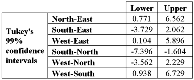
Exhibit 13.5 A police chief wants to determine if crime rates are different for four different areas of the city (East(1),West(2),North(3),and South(4)sides),and obtains data on the number of crimes per day in each area.The one-way ANOVA table and Tukey's confidence intervals are shown below. 
 Refer to Exhibit 13.5.At the 1% significance level,the conclusion for the hypothesis test is:
A)Reject the null hypothesis,not all mean number of crimes are equal
B)Do not reject the null hypothesis,not all mean number of crimes are equal
C)Reject the null hypothesis,cannot conclude that not all mean number of crimes are equal
D)Do not reject the null hypothesis,cannot conclude that not all mean number of crimes are equal
Refer to Exhibit 13.5.At the 1% significance level,the conclusion for the hypothesis test is:A)Reject the null hypothesis,not all mean number of crimes are equal
B)Do not reject the null hypothesis,not all mean number of crimes are equal
C)Reject the null hypothesis,cannot conclude that not all mean number of crimes are equal
D)Do not reject the null hypothesis,cannot conclude that not all mean number of crimes are equal
سؤال
Exhibit 13.5 A police chief wants to determine if crime rates are different for four different areas of the city (East(1),West(2),North(3),and South(4)sides),and obtains data on the number of crimes per day in each area.The one-way ANOVA table and Tukey's confidence intervals are shown below. 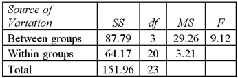
 Refer to Exhibit 13.5.The competing hypotheses about the mean crime rates are:
A)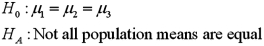
B)
C)
D)
Refer to Exhibit 13.5.The competing hypotheses about the mean crime rates are:A)
B)
C)
D)
سؤال
Exhibit 13.3 The ANOVA test performed for Exhibit 13.2 determined that not all mean commute times across the four cities are equal.However,it did not indicate which means differed.To find out which population means differ requires further analysis of the direction and the statistical significance of the difference between paired population means.Fisher 95% confidence intervals are shown below.  Refer to Exhibit 13.3.Which of the following is the
  value used to calculate the Fisher 95% confidence intervals?
A)1.725
B)2.086
C)2.080
D)2.090
Refer to Exhibit 13.3.Which of the following is the value used to calculate the Fisher 95% confidence intervals?A)1.725
B)2.086
C)2.080
D)2.090
سؤال
Exhibit 13.6 A researcher wants to understand how annual mortgage payment (in dollars)depends on income level and zonal location using a two-way ANOVA without interaction.The data and an incomplete ANOVA table are shown below. 
 Refer to Exhibit 13.6.At the 1% significance level,the conclusion for the hypothesis test about factor B is:
A)Do not reject the null hypothesis,the average mortgage payments differ by zonal location
B)Do not reject the null hypothesis,cannot conclude the average mortgage payments differ by zonal location
C)Reject the null hypothesis,the average mortgage payments differ by zonal location
D)Reject the null hypothesis,cannot conclude the average mortgage payments differ by zonal location
Refer to Exhibit 13.6.At the 1% significance level,the conclusion for the hypothesis test about factor B is:A)Do not reject the null hypothesis,the average mortgage payments differ by zonal location
B)Do not reject the null hypothesis,cannot conclude the average mortgage payments differ by zonal location
C)Reject the null hypothesis,the average mortgage payments differ by zonal location
D)Reject the null hypothesis,cannot conclude the average mortgage payments differ by zonal location
سؤال
Exhibit 13.6 A researcher wants to understand how annual mortgage payment (in dollars)depends on income level and zonal location using a two-way ANOVA without interaction.The data and an incomplete ANOVA table are shown below. 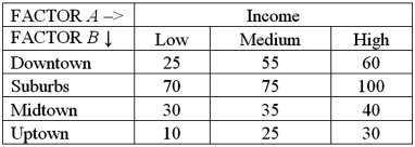
 Refer to Exhibit 13.6.Which of the following is the value of the test statistic for factor A?
A)4.76
B)5.14
C)9.41
D)32.86
Refer to Exhibit 13.6.Which of the following is the value of the test statistic for factor A?A)4.76
B)5.14
C)9.41
D)32.86
سؤال
Exhibit 13.5 A police chief wants to determine if crime rates are different for four different areas of the city (East(1),West(2),North(3),and South(4)sides),and obtains data on the number of crimes per day in each area.The one-way ANOVA table and Tukey's confidence intervals are shown below. 
 Refer to Exhibit 13.5.At the 1% significance level,the conclusion from Tukey's confidence intervals is:
A)Cannot conclude the mean number of crimes differs for West and East
B)Cannot conclude the mean number of crimes differs for West and South
C)Cannot conclude the mean number of crimes differs for South and North
D)Cannot conclude the mean number of crimes differs for West and North
Refer to Exhibit 13.5.At the 1% significance level,the conclusion from Tukey's confidence intervals is:A)Cannot conclude the mean number of crimes differs for West and East
B)Cannot conclude the mean number of crimes differs for West and South
C)Cannot conclude the mean number of crimes differs for South and North
D)Cannot conclude the mean number of crimes differs for West and North
سؤال
Exhibit 13.3 The ANOVA test performed for Exhibit 13.2 determined that not all mean commute times across the four cities are equal.However,it did not indicate which means differed.To find out which population means differ requires further analysis of the direction and the statistical significance of the difference between paired population means.Fisher 95% confidence intervals are shown below. 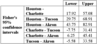 Refer to Exhibit 13.3.Which of these pair of cities shows no significant difference in average commute times to work?
A)Houston,Akron
B)Charlotte,Akron
C)Charlotte,Tucson
D)Houston,Tucson
Refer to Exhibit 13.3.Which of these pair of cities shows no significant difference in average commute times to work?A)Houston,Akron
B)Charlotte,Akron
C)Charlotte,Tucson
D)Houston,Tucson
سؤال
Exhibit 13.5 A police chief wants to determine if crime rates are different for four different areas of the city (East(1),West(2),North(3),and South(4)sides),and obtains data on the number of crimes per day in each area.The one-way ANOVA table and Tukey's confidence intervals are shown below. 
 Refer to Exhibit 13.5.At the 1% significance level,the critical value is:
A)2.38
B)3.10
C)3.86
D)4.94
Refer to Exhibit 13.5.At the 1% significance level,the critical value is:A)2.38
B)3.10
C)3.86
D)4.94
سؤال
Exhibit 13.6 A researcher wants to understand how annual mortgage payment (in dollars)depends on income level and zonal location using a two-way ANOVA without interaction.The data and an incomplete ANOVA table are shown below. 
 Refer to Exhibit 13.6.At the 1% significance level,the critical value for the hypothesis test about factor B is:
A)3.29
B)4.76
C)6.60
D)9.78
Refer to Exhibit 13.6.At the 1% significance level,the critical value for the hypothesis test about factor B is:A)3.29
B)4.76
C)6.60
D)9.78
سؤال
Exhibit 13.6 A researcher wants to understand how annual mortgage payment (in dollars)depends on income level and zonal location using a two-way ANOVA without interaction.The data and an incomplete ANOVA table are shown below. 
 Refer to Exhibit 13.6.Which of the following is the value of the test statistic for factor B?
A)4.76
B)5.14
C)9.41
D)32.86
Refer to Exhibit 13.6.Which of the following is the value of the test statistic for factor B?A)4.76
B)5.14
C)9.41
D)32.86
سؤال
Exhibit 13.4 The ANOVA test performed for Exhibit 13.2 determined that not all mean commute times across the four cities are equal.However,it did not indicate which means differed.To find out which population means differ requires further analysis of the direction and the statistical significance of the difference between paired population means.Tukey 95% confidence intervals are shown below.  Refer to Exhibit 13.4.Which of these pair of cities shows a significant difference in average commute times to work?
A)Houston,Akron
B)Charlotte,Akron
C)Charlotte,Tucson
D)Akron,Tucson
Refer to Exhibit 13.4.Which of these pair of cities shows a significant difference in average commute times to work?A)Houston,Akron
B)Charlotte,Akron
C)Charlotte,Tucson
D)Akron,Tucson
سؤال
Exhibit 13.5 A police chief wants to determine if crime rates are different for four different areas of the city (East(1),West(2),North(3),and South(4)sides),and obtains data on the number of crimes per day in each area.The one-way ANOVA table and Tukey's confidence intervals are shown below. 
 Refer to Exhibit 13.5.The degrees of freedom for the hypothesis test are:
A)4,20
B)3,23
C)3,20
D)4,23
Refer to Exhibit 13.5.The degrees of freedom for the hypothesis test are:A)4,20
B)3,23
C)3,20
D)4,23
سؤال
Exhibit 13.4 The ANOVA test performed for Exhibit 13.2 determined that not all mean commute times across the four cities are equal.However,it did not indicate which means differed.To find out which population means differ requires further analysis of the direction and the statistical significance of the difference between paired population means.Tukey 95% confidence intervals are shown below.  Refer to Exhibit 13.4.Which of the following is the studentized range value with α = 0.05 for Tukey's HSD method?
A)5.02
B)3.58
C)3.96
D)4.64
Refer to Exhibit 13.4.Which of the following is the studentized range value with α = 0.05 for Tukey's HSD method?A)5.02
B)3.58
C)3.96
D)4.64
سؤال
Exhibit 13.6 A researcher wants to understand how annual mortgage payment (in dollars)depends on income level and zonal location using a two-way ANOVA without interaction.The data and an incomplete ANOVA table are shown below. 
 Refer to Exhibit 13.6.At the 5% significance level,the critical value for the hypothesis test about factor A is:
A)3.46
B)5.14
C)7.26
D)10.92
Refer to Exhibit 13.6.At the 5% significance level,the critical value for the hypothesis test about factor A is:A)3.46
B)5.14
C)7.26
D)10.92
سؤال
Exhibit 13.4 The ANOVA test performed for Exhibit 13.2 determined that not all mean commute times across the four cities are equal.However,it did not indicate which means differed.To find out which population means differ requires further analysis of the direction and the statistical significance of the difference between paired population means.Tukey 95% confidence intervals are shown below.  Refer to Exhibit 13.4.The conclusion of the Tukey confidence intervals is:
A)The mean commute time in Houston is different from the mean commute time in Charlotte,Tucson,and Akron.
B)The mean commute time in Charlotte is different from the mean commute time in Houston,Tucson,and Akron.
C)The mean commute time in Tucson is different from the mean commute time in Houston,Charlotte,and Akron.
D)The mean commute time in Akron is different from the mean time in Houston,Charlotte,and Tucson.
Refer to Exhibit 13.4.The conclusion of the Tukey confidence intervals is:A)The mean commute time in Houston is different from the mean commute time in Charlotte,Tucson,and Akron.
B)The mean commute time in Charlotte is different from the mean commute time in Houston,Tucson,and Akron.
C)The mean commute time in Tucson is different from the mean commute time in Houston,Charlotte,and Akron.
D)The mean commute time in Akron is different from the mean time in Houston,Charlotte,and Tucson.
سؤال
Exhibit 13.6 A researcher wants to understand how annual mortgage payment (in dollars)depends on income level and zonal location using a two-way ANOVA without interaction.The data and an incomplete ANOVA table are shown below. 
 Refer to Exhibit 13.6.Which of the following are the total degrees of freedom?
A)10
B)11
C)12
D)6
Refer to Exhibit 13.6.Which of the following are the total degrees of freedom?A)10
B)11
C)12
D)6
سؤال
Exhibit 13.8 A market researcher is studying the spending habits of people across age groups.The amount of money spent by each individual is classified by spending category (Dining out,Shopping or Electronics)and generation (Gen-X,Gen-Y,Gen-Z or Baby Boomers).The data and an incomplete ANOVA table are shown below. 
 Refer to Exhibit 13.8.The value of SSE is:
A)46,869
B)159,860
C)116,767
D)1,321,831
Refer to Exhibit 13.8.The value of SSE is:A)46,869
B)159,860
C)116,767
D)1,321,831
سؤال
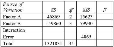
Exhibit 13.7 A market researcher is studying the spending habits of people across age groups.The amount of money spent by each individual is classified by spending category (Dining out,Shopping or Electronics)and generation (Gen-X,Gen-Y,Gen-Z or Baby Boomers).An incomplete ANOVA table are shown below.  Refer to Exhibit 13.7.Which of the following is the value of MSE?
A)15,623
B)79,930
C)37,170
D)1,321,831
Refer to Exhibit 13.7.Which of the following is the value of MSE?A)15,623
B)79,930
C)37,170
D)1,321,831
سؤال
Exhibit 13.8 A market researcher is studying the spending habits of people across age groups.The amount of money spent by each individual is classified by spending category (Dining out,Shopping or Electronics)and generation (Gen-X,Gen-Y,Gen-Z or Baby Boomers).The data and an incomplete ANOVA table are shown below. 
 Refer to Exhibit 13.8.The degrees of freedom for the interaction and the error are:
A)6,24
B)6,30
C)24,6
D)30,6
Refer to Exhibit 13.8.The degrees of freedom for the interaction and the error are:A)6,24
B)6,30
C)24,6
D)30,6
سؤال
A farmer plants tomato seeds into four different plots.In each plot,there is a different fertilizer treatment that is applied to the soil.After three weeks,he measures the height of each tomato plant from each of the four plots.The data he collects is given shown below. 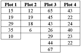
A)Construct an ANOVA table.
B)Set up the competing hypothesis to test whether there are some differences in the mean heights between the different plots/fertilizers.
C)At the 5% significance level,what is the conclusion to the test?
D)Consider the sample standard deviations for each plot.Which of the assumptions might be violated?
سؤال
Exhibit 13.7 A market researcher is studying the spending habits of people across age groups.The amount of money spent by each individual is classified by spending category (Dining out,Shopping or Electronics)and generation (Gen-X,Gen-Y,Gen-Z or Baby Boomers).An incomplete ANOVA table are shown below.  Refer to Exhibit 13.7.How many degrees of freedom are there for factors A and B?
A)2,3
B)3,4
C)3,6
D)2,4
Refer to Exhibit 13.7.How many degrees of freedom are there for factors A and B?A)2,3
B)3,4
C)3,6
D)2,4
سؤال
Exhibit 13.8 A market researcher is studying the spending habits of people across age groups.The amount of money spent by each individual is classified by spending category (Dining out,Shopping or Electronics)and generation (Gen-X,Gen-Y,Gen-Z or Baby Boomers).The data and an incomplete ANOVA table are shown below. 
 Refer to Exhibit 13.8.At the 5% significance level,the critical value for the test about the interaction is:
A)2.04
B)2.51
C)2.99
D)3.67
Refer to Exhibit 13.8.At the 5% significance level,the critical value for the test about the interaction is:A)2.04
B)2.51
C)2.99
D)3.67
سؤال
Exhibit 13.8 A market researcher is studying the spending habits of people across age groups.The amount of money spent by each individual is classified by spending category (Dining out,Shopping or Electronics)and generation (Gen-X,Gen-Y,Gen-Z or Baby Boomers).The data and an incomplete ANOVA table are shown below. 
 Refer to Exhibit 13.8.For the analysis with an interaction between spending category and generation,the first hypothesis test to conduct should be about the:
A)Average spending across spending
B)The interaction between spending and generation
C)Average spending across generation
D)Both the average spending across spending and generation
Refer to Exhibit 13.8.For the analysis with an interaction between spending category and generation,the first hypothesis test to conduct should be about the:A)Average spending across spending
B)The interaction between spending and generation
C)Average spending across generation
D)Both the average spending across spending and generation
سؤال
Exhibit 13.8 A market researcher is studying the spending habits of people across age groups.The amount of money spent by each individual is classified by spending category (Dining out,Shopping or Electronics)and generation (Gen-X,Gen-Y,Gen-Z or Baby Boomers).The data and an incomplete ANOVA table are shown below. 
 Refer to Exhibit 13.8.The value of MSAB is:
A)983,335
B)116,767
C)159,860
D)166,389
Refer to Exhibit 13.8.The value of MSAB is:A)983,335
B)116,767
C)159,860
D)166,389
سؤال
Exhibit 13.7 A market researcher is studying the spending habits of people across age groups.The amount of money spent by each individual is classified by spending category (Dining out,Shopping or Electronics)and generation (Gen-X,Gen-Y,Gen-Z or Baby Boomers).An incomplete ANOVA table are shown below.  Refer to Exhibit 13.7.At the 5% significance level,the conclusion of the hypothesis test for factor A is:
A)Do not reject the null hypothesis,cannot conclude the average amount spent differs by spending category
B)Do not reject the null hypothesis,the average amount spent differs by spending category
C)Reject the null hypothesis,cannot conclude the average amount spent differs by spending category
D)Reject the null hypothesis,the average amount spent differs by spending category
Refer to Exhibit 13.7.At the 5% significance level,the conclusion of the hypothesis test for factor A is:A)Do not reject the null hypothesis,cannot conclude the average amount spent differs by spending category
B)Do not reject the null hypothesis,the average amount spent differs by spending category
C)Reject the null hypothesis,cannot conclude the average amount spent differs by spending category
D)Reject the null hypothesis,the average amount spent differs by spending category
سؤال
Exhibit 13.7 A market researcher is studying the spending habits of people across age groups.The amount of money spent by each individual is classified by spending category (Dining out,Shopping or Electronics)and generation (Gen-X,Gen-Y,Gen-Z or Baby Boomers).An incomplete ANOVA table are shown below.  Refer to Exhibit 13.7.At the 5% significance level,the critical value for the hypothesis test about factor B is:
A)2.28
B)2.92
C)3.59
D)4.51
Refer to Exhibit 13.7.At the 5% significance level,the critical value for the hypothesis test about factor B is:A)2.28
B)2.92
C)3.59
D)4.51
سؤال
Exhibit 13.7 A market researcher is studying the spending habits of people across age groups.The amount of money spent by each individual is classified by spending category (Dining out,Shopping or Electronics)and generation (Gen-X,Gen-Y,Gen-Z or Baby Boomers).An incomplete ANOVA table are shown below.  Refer to Exhibit 13.7.At the 5% significance level,the critical value for the hypothesis test about factor A is:
A)2.49
B)3.32
C)4.18
D)5.39
Refer to Exhibit 13.7.At the 5% significance level,the critical value for the hypothesis test about factor A is:A)2.49
B)3.32
C)4.18
D)5.39
سؤال
Exhibit 13.8 A market researcher is studying the spending habits of people across age groups.The amount of money spent by each individual is classified by spending category (Dining out,Shopping or Electronics)and generation (Gen-X,Gen-Y,Gen-Z or Baby Boomers).The data and an incomplete ANOVA table are shown below. 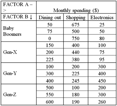
 Refer to Exhibit 13.8.For the interaction,the value of the test statistic is:
A)34.20
B)16.43
C)3.21
D)24
Refer to Exhibit 13.8.For the interaction,the value of the test statistic is:A)34.20
B)16.43
C)3.21
D)24
سؤال
Exhibit 13.7 A market researcher is studying the spending habits of people across age groups.The amount of money spent by each individual is classified by spending category (Dining out,Shopping or Electronics)and generation (Gen-X,Gen-Y,Gen-Z or Baby Boomers).An incomplete ANOVA table are shown below.  Refer to Exhibit 13.7.For factor A,the value of the test statistic is:
A)3.21
B)2
C)16.43
D)3
Refer to Exhibit 13.7.For factor A,the value of the test statistic is:A)3.21
B)2
C)16.43
D)3
سؤال
Exhibit 13.9 Psychology students want to determine if there are differences between the ability of business majors and science majors to solve various types of analytic problems.They conduct an experiment and record the amount of time it takes to complete each analytic problem.The following two-way ANOVA table summarizes their findings. 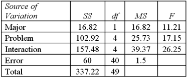 Refer to Exhibit 13.9.At the 5% significance level,the conclusion for the hypothesis test about the interaction term is:
A)Do not reject the null hypothesis,there is no evidence of an interaction effect between major and problem type
B)Reject the null hypothesis,there is no evidence of an interaction effect between major and problem type
C)Reject the null hypothesis,there is evidence of an interaction effect between major and problem type
D)Do not reject the null hypothesis,there is evidence of an interaction effect between major and problem type
Refer to Exhibit 13.9.At the 5% significance level,the conclusion for the hypothesis test about the interaction term is:A)Do not reject the null hypothesis,there is no evidence of an interaction effect between major and problem type
B)Reject the null hypothesis,there is no evidence of an interaction effect between major and problem type
C)Reject the null hypothesis,there is evidence of an interaction effect between major and problem type
D)Do not reject the null hypothesis,there is evidence of an interaction effect between major and problem type
سؤال
Exhibit 13.7 A market researcher is studying the spending habits of people across age groups.The amount of money spent by each individual is classified by spending category (Dining out,Shopping or Electronics)and generation (Gen-X,Gen-Y,Gen-Z or Baby Boomers).An incomplete ANOVA table are shown below.  Refer to Exhibit 13.7.Which of the following is the value of MSA?
A)15,623
B)79,930
C)37,170
D)1,321,831
Refer to Exhibit 13.7.Which of the following is the value of MSA?A)15,623
B)79,930
C)37,170
D)1,321,831
سؤال
Exhibit 13.8 A market researcher is studying the spending habits of people across age groups.The amount of money spent by each individual is classified by spending category (Dining out,Shopping or Electronics)and generation (Gen-X,Gen-Y,Gen-Z or Baby Boomers).The data and an incomplete ANOVA table are shown below. 
 Refer to Exhibit 13.8.At the 5% significance level,the conclusion for the hypothesis test about the interaction term is:
A)Do not reject the null hypothesis,there is evidence of an interaction effect between spending category and generation
B)Reject the null hypothesis,there is evidence of an interaction effect between spending category and generation
C)Reject the null hypothesis,there is no evidence of an interaction effect between spending category and generation
D)Do not reject the null hypothesis,there is no evidence of an interaction effect between spending category and generation
Refer to Exhibit 13.8.At the 5% significance level,the conclusion for the hypothesis test about the interaction term is:A)Do not reject the null hypothesis,there is evidence of an interaction effect between spending category and generation
B)Reject the null hypothesis,there is evidence of an interaction effect between spending category and generation
C)Reject the null hypothesis,there is no evidence of an interaction effect between spending category and generation
D)Do not reject the null hypothesis,there is no evidence of an interaction effect between spending category and generation
سؤال
Exhibit 13.9 Psychology students want to determine if there are differences between the ability of business majors and science majors to solve various types of analytic problems.They conduct an experiment and record the amount of time it takes to complete each analytic problem.The following two-way ANOVA table summarizes their findings.  Refer to Exhibit 13.9.The number of different analytic problems the students solved is:
A)1
B)2
C)4
D)5
Refer to Exhibit 13.9.The number of different analytic problems the students solved is:A)1
B)2
C)4
D)5
سؤال
Exhibit 13.8 A market researcher is studying the spending habits of people across age groups.The amount of money spent by each individual is classified by spending category (Dining out,Shopping or Electronics)and generation (Gen-X,Gen-Y,Gen-Z or Baby Boomers).The data and an incomplete ANOVA table are shown below. 
 Refer to Exhibit 13.8.The conclusion for the hypothesis test about the interaction term is:
A)
B)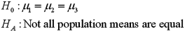
C)
D)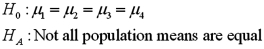
Refer to Exhibit 13.8.The conclusion for the hypothesis test about the interaction term is:A)
B)
C)
D)
سؤال
Exhibit 13.7 A market researcher is studying the spending habits of people across age groups.The amount of money spent by each individual is classified by spending category (Dining out,Shopping or Electronics)and generation (Gen-X,Gen-Y,Gen-Z or Baby Boomers).An incomplete ANOVA table are shown below. 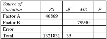 Refer to Exhibit 13.7.At the 5% significance level,the conclusion of the hypothesis test for Factor B is:
A)Do not reject the null hypothesis,cannot conclude the average amount spent differs by generation
B)Do not reject the null hypothesis,the average amount spent differs by generation
C)Reject the null hypothesis,cannot conclude the average amount spent differs by generation
D)Reject the null hypothesis,the average amount spent differs by generation
Refer to Exhibit 13.7.At the 5% significance level,the conclusion of the hypothesis test for Factor B is:A)Do not reject the null hypothesis,cannot conclude the average amount spent differs by generation
B)Do not reject the null hypothesis,the average amount spent differs by generation
C)Reject the null hypothesis,cannot conclude the average amount spent differs by generation
D)Reject the null hypothesis,the average amount spent differs by generation
سؤال
Exhibit 13.7 A market researcher is studying the spending habits of people across age groups.The amount of money spent by each individual is classified by spending category (Dining out,Shopping or Electronics)and generation (Gen-X,Gen-Y,Gen-Z or Baby Boomers).An incomplete ANOVA table are shown below.  Refer to Exhibit 13.7.Which of the following is the value of SSB?
A)46,869
B)159,860
C)1,115,101
D)1,321,831
Refer to Exhibit 13.7.Which of the following is the value of SSB?A)46,869
B)159,860
C)1,115,101
D)1,321,831

فتح الحزمة
قم بالتسجيل لفتح البطاقات في هذه المجموعة!
Unlock Deck
Unlock Deck
1/89
العب
ملء الشاشة (f)
Deck 13: Analysis of Variance
1
Fisher's 100(1 - α)% confidence interval for the difference between two population means μi - μj is:
A)
B)
C)
D)
A)
B)
C)
D)
2
If the amount of variability between treatments is significantly greater than the amount of variability within treatments,then:
A)reject the null hypothesis of equal population means
B)do not reject the null hypothesis of equal population means
C)conclude that the ratio of between-treatments variability to within-treatments variability is significantly less than 1
D)perform further analysis using the two-way ANOVA with interaction
reject the null hypothesis of equal population means
3
If units within each block are randomly assigned to each of the treatments,then the design of the experiment is referred to as a completely randomized design.
False
4
Identify the assumption that is not applicable for a one-way ANOVA test.
A)The populations are normally distributed
B)The population standard deviations are not all equal
C)The samples are selected independently
D)The sample is drawn at random from each population
A)The populations are normally distributed
B)The population standard deviations are not all equal
C)The samples are selected independently
D)The sample is drawn at random from each population
فتح الحزمة
افتح القفل للوصول البطاقات البالغ عددها 89 في هذه المجموعة.
فتح الحزمة
k this deck
5
When using Fisher's least significant difference (LSD)method at some stated significance level,the probability of committing a Type I error increases as the number of:
A)pairwise comparisons decreases
B)pairwise comparisons increases
C)sample size increases
D)treatments decreases
A)pairwise comparisons decreases
B)pairwise comparisons increases
C)sample size increases
D)treatments decreases
فتح الحزمة
افتح القفل للوصول البطاقات البالغ عددها 89 في هذه المجموعة.
فتح الحزمة
k this deck
6
The interaction test is performed before making any conclusions based on the tests for the main effects.
فتح الحزمة
افتح القفل للوصول البطاقات البالغ عددها 89 في هذه المجموعة.
فتح الحزمة
k this deck
7
The between-treatments variability is the estimate of σ2 which is based on the variability due to chance.
فتح الحزمة
افتح القفل للوصول البطاقات البالغ عددها 89 في هذه المجموعة.
فتح الحزمة
k this deck
8
In general,blocks are the levels at which we hold an integral factor fixed,so that we can measure its contribution to the variation within the samples.
فتح الحزمة
افتح القفل للوصول البطاقات البالغ عددها 89 في هذه المجموعة.
فتح الحزمة
k this deck
9
When the null hypothesis is rejected in an ANOVA test,Fisher's least significant difference method is superior to Tukey's honestly significant differences method to determine which population means differ.
فتح الحزمة
افتح القفل للوصول البطاقات البالغ عددها 89 في هذه المجموعة.
فتح الحزمة
k this deck
10
Fisher's least difference (LSD)method is applied when the:
A)ANOVA test has not rejected the null hypothesis of equal population means
B)ANOVA test has rejected the null hypothesis of equal population means
C)Two-sample t test is not applicable
D)None of the above
A)ANOVA test has not rejected the null hypothesis of equal population means
B)ANOVA test has rejected the null hypothesis of equal population means
C)Two-sample t test is not applicable
D)None of the above
فتح الحزمة
افتح القفل للوصول البطاقات البالغ عددها 89 في هذه المجموعة.
فتح الحزمة
k this deck
11
When two factors interact,the effect of one factor on the population mean depends upon the specific value or level present for the other factor.
فتح الحزمة
افتح القفل للوصول البطاقات البالغ عددها 89 في هذه المجموعة.
فتح الحزمة
k this deck
12
One-Way ANOVA analyzes the effect of one factor on the population mean.It is based on a:
A)randomized block design
B)completely randomized design
C)factorial design
D)balanced incomplete block design
A)randomized block design
B)completely randomized design
C)factorial design
D)balanced incomplete block design
فتح الحزمة
افتح القفل للوصول البطاقات البالغ عددها 89 في هذه المجموعة.
فتح الحزمة
k this deck
13
We use ANOVA to test for differences between population means by examining the amount of variability between the samples relative to the amount of variability within the samples.
فتح الحزمة
افتح القفل للوصول البطاقات البالغ عددها 89 في هذه المجموعة.
فتح الحزمة
k this deck
14
ANOVA is a statistical technique used to determine if differences exist between the means of two populations.
فتح الحزمة
افتح القفل للوصول البطاقات البالغ عددها 89 في هذه المجموعة.
فتح الحزمة
k this deck
15
One-way ANOVA analyzes the effect of one factor on the population mean and it is based on a completely randomized design.
فتح الحزمة
افتح القفل للوصول البطاقات البالغ عددها 89 في هذه المجموعة.
فتح الحزمة
k this deck
16
Which of the following is the correct interpretation of the Fisher's 100(1 - α)% confidence interval for μi - μj?
A)If the interval includes the value zero,the null hypothesis,that H0: μi - μj = 0,is rejected for at α level of significance
B)If the interval does not include the value zero,the null hypothesis,that H0: μi - μj = 0,is rejected at 100(1 - α)% level of significance
C)If the interval does not include the value zero,the null hypothesis,that H0: μi - μj = 0,is rejected at α level of significance
D)If the interval includes the value zero,the null hypothesis,that H0: μi - μj = 0,is rejected at 100(1 - α)% level of significance
فتح الحزمة
افتح القفل للوصول البطاقات البالغ عددها 89 في هذه المجموعة.
فتح الحزمة
k this deck
17
When using Fisher's LSD method at some stated significance level α,the probability of committing a Type I error increases as the number of pairwise comparisons increases.
فتح الحزمة
افتح القفل للوصول البطاقات البالغ عددها 89 في هذه المجموعة.
فتح الحزمة
k this deck
18
If there are five treatments under study,the number of pairwise comparisons is:
A)15
B)5
C)20
D)10
A)15
B)5
C)20
D)10
فتح الحزمة
افتح القفل للوصول البطاقات البالغ عددها 89 في هذه المجموعة.
فتح الحزمة
k this deck
19
The variability due to chance,also known as within-treatments variability,is the estimate of σ2 which is based on the:
A)variability of the data across different samples
B)consistency of the data within each sample
C)variability of the data within each sample
D)reliability of the data within each sample
A)variability of the data across different samples
B)consistency of the data within each sample
C)variability of the data within each sample
D)reliability of the data within each sample
فتح الحزمة
افتح القفل للوصول البطاقات البالغ عددها 89 في هذه المجموعة.
فتح الحزمة
k this deck
20
Between-treatments variability is based on a weighted sum of squared differences between the:
A)population variances and the overall mean of the data set
B)sample means and the overall mean of the data set
C)sample variances and the overall mean of the data set
D)population means and the overall mean of the data set
A)population variances and the overall mean of the data set
B)sample means and the overall mean of the data set
C)sample variances and the overall mean of the data set
D)population means and the overall mean of the data set
فتح الحزمة
افتح القفل للوصول البطاقات البالغ عددها 89 في هذه المجموعة.
فتح الحزمة
k this deck
21
Exhibit 13.2 A researcher with Ministry of Transportation is commissioned to study the drive times to work (one-way)for U.S.cities.The underlying hypothesis is that average commute times are different across cities.To test the hypothesis,the researcher randomly selects six people from each of the four cities and records their one-way commute times to work.Refer to the below data on one-way commute time (in minutes)to work.Note that the grand mean is 36.625. Refer to Exhibit 13.2.Which of the following is the sum of squared errors?
A)264.29
B)5,285.83
C)18,567.63
D)13,281.79
Refer to Exhibit 13.2.Which of the following is the sum of squared errors?A)264.29
B)5,285.83
C)18,567.63
D)13,281.79
فتح الحزمة
افتح القفل للوصول البطاقات البالغ عددها 89 في هذه المجموعة.
فتح الحزمة
k this deck
22
If units with each block are randomly assigned to each of the treatments,then the design of the experiment is referred to as a:
A)factorial design
B)completely randomized design
C)randomized block design
D)balanced incomplete block design
A)factorial design
B)completely randomized design
C)randomized block design
D)balanced incomplete block design
فتح الحزمة
افتح القفل للوصول البطاقات البالغ عددها 89 في هذه المجموعة.
فتح الحزمة
k this deck
23
Tukey's 100(1 - α)% confidence interval for the difference between two population means μi - μj for balanced data is given by ____.
A)
B)
C)
D)
A)
B)
C)
D)
فتح الحزمة
افتح القفل للوصول البطاقات البالغ عددها 89 في هذه المجموعة.
فتح الحزمة
k this deck
24
Exhibit 13.2 A researcher with Ministry of Transportation is commissioned to study the drive times to work (one-way)for U.S.cities.The underlying hypothesis is that average commute times are different across cities.To test the hypothesis,the researcher randomly selects six people from each of the four cities and records their one-way commute times to work.Refer to the below data on one-way commute time (in minutes)to work.Note that the grand mean is 36.625. Refer to Exhibit 13.2.At the 5% significance level,the critical value is:
A)2.38
B)3.10
C)3.86
D)4.94
Refer to Exhibit 13.2.At the 5% significance level,the critical value is:A)2.38
B)3.10
C)3.86
D)4.94
فتح الحزمة
افتح القفل للوصول البطاقات البالغ عددها 89 في هذه المجموعة.
فتح الحزمة
k this deck
25
One of the disadvantages of Fisher's least difference (LSD)method is that the probability of committing a:
A)Type II error increases as the number of pairwise comparisons increases.
B)Type I error increases as the number of pairwise comparisons decreases.
C)Type II error increases as the number of pairwise comparisons decreases.
D)Type I error increases as the number of pairwise comparisons increases.
A)Type II error increases as the number of pairwise comparisons increases.
B)Type I error increases as the number of pairwise comparisons decreases.
C)Type II error increases as the number of pairwise comparisons decreases.
D)Type I error increases as the number of pairwise comparisons increases.
فتح الحزمة
افتح القفل للوصول البطاقات البالغ عددها 89 في هذه المجموعة.
فتح الحزمة
k this deck
26
In a two-way ANOVA test,how many null hypotheses are tested?
A)1
B)1 or 2
C)2 or 3
D)More than 3
A)1
B)1 or 2
C)2 or 3
D)More than 3
فتح الحزمة
افتح القفل للوصول البطاقات البالغ عددها 89 في هذه المجموعة.
فتح الحزمة
k this deck
27
If the interaction between two factors is not significant,the next tests to be done are:
A)None,the analysis is complete.
B)None,gather more data.
C)Tests about the population means of factor A or factor B using two-way ANOVA without interaction.
D)Tukey's confidence intervals.
A)None,the analysis is complete.
B)None,gather more data.
C)Tests about the population means of factor A or factor B using two-way ANOVA without interaction.
D)Tukey's confidence intervals.
فتح الحزمة
افتح القفل للوصول البطاقات البالغ عددها 89 في هذه المجموعة.
فتح الحزمة
k this deck
28
Exhibit 13.2 A researcher with Ministry of Transportation is commissioned to study the drive times to work (one-way)for U.S.cities.The underlying hypothesis is that average commute times are different across cities.To test the hypothesis,the researcher randomly selects six people from each of the four cities and records their one-way commute times to work.Refer to the below data on one-way commute time (in minutes)to work.Note that the grand mean is 36.625. Refer to Exhibit 13.2.The conclusion for the hypothesis test is:
A)Reject the null hypothesis,cannot conclude that not all mean commute times are equal
B)Do not reject the null hypothesis,cannot conclude that not all mean commute times are equal
C)Reject the null hypothesis,not all mean commute times are equal
D)Do not reject the null hypothesis,not all mean commute times are equal
Refer to Exhibit 13.2.The conclusion for the hypothesis test is:A)Reject the null hypothesis,cannot conclude that not all mean commute times are equal
B)Do not reject the null hypothesis,cannot conclude that not all mean commute times are equal
C)Reject the null hypothesis,not all mean commute times are equal
D)Do not reject the null hypothesis,not all mean commute times are equal
فتح الحزمة
افتح القفل للوصول البطاقات البالغ عددها 89 في هذه المجموعة.
فتح الحزمة
k this deck
29
Exhibit 13.2 A researcher with Ministry of Transportation is commissioned to study the drive times to work (one-way)for U.S.cities.The underlying hypothesis is that average commute times are different across cities.To test the hypothesis,the researcher randomly selects six people from each of the four cities and records their one-way commute times to work.Refer to the below data on one-way commute time (in minutes)to work.Note that the grand mean is 36.625. Refer to Exhibit 13.2.Which of the following is the sum of squares due to treatments?
A)5,285.83
B)13,281.79
C)18,567.63
D)4,427.26
Refer to Exhibit 13.2.Which of the following is the sum of squares due to treatments?A)5,285.83
B)13,281.79
C)18,567.63
D)4,427.26
فتح الحزمة
افتح القفل للوصول البطاقات البالغ عددها 89 في هذه المجموعة.
فتح الحزمة
k this deck
30
Exhibit 13.2 A researcher with Ministry of Transportation is commissioned to study the drive times to work (one-way)for U.S.cities.The underlying hypothesis is that average commute times are different across cities.To test the hypothesis,the researcher randomly selects six people from each of the four cities and records their one-way commute times to work.Refer to the below data on one-way commute time (in minutes)to work.Note that the grand mean is 36.625. Refer to Exhibit 13.2.The value of the test statistic is:
A)0.06
B)0.40
C)2.51
D)16.75
Refer to Exhibit 13.2.The value of the test statistic is:A)0.06
B)0.40
C)2.51
D)16.75
فتح الحزمة
افتح القفل للوصول البطاقات البالغ عددها 89 في هذه المجموعة.
فتح الحزمة
k this deck
31
Exhibit 13.2 A researcher with Ministry of Transportation is commissioned to study the drive times to work (one-way)for U.S.cities.The underlying hypothesis is that average commute times are different across cities.To test the hypothesis,the researcher randomly selects six people from each of the four cities and records their one-way commute times to work.Refer to the below data on one-way commute time (in minutes)to work.Note that the grand mean is 36.625. Refer to Exhibit 13.2.Based on the sample standard deviation,the one-way ANOVA assumption which is likely not met is:
A)The populations are normally distributed
B)The population standard deviations are assumed to be equal
C)The samples are independent
D)None of the above
Refer to Exhibit 13.2.Based on the sample standard deviation,the one-way ANOVA assumption which is likely not met is:A)The populations are normally distributed
B)The population standard deviations are assumed to be equal
C)The samples are independent
D)None of the above
فتح الحزمة
افتح القفل للوصول البطاقات البالغ عددها 89 في هذه المجموعة.
فتح الحزمة
k this deck
32
Exhibit 13.2 A researcher with Ministry of Transportation is commissioned to study the drive times to work (one-way)for U.S.cities.The underlying hypothesis is that average commute times are different across cities.To test the hypothesis,the researcher randomly selects six people from each of the four cities and records their one-way commute times to work.Refer to the below data on one-way commute time (in minutes)to work.Note that the grand mean is 36.625. Refer to Exhibit 13.2.The competing hypotheses about the mean commute times are:
A)
B)
C)
D)
Refer to Exhibit 13.2.The competing hypotheses about the mean commute times are:A)
B)
C)
D)
فتح الحزمة
افتح القفل للوصول البطاقات البالغ عددها 89 في هذه المجموعة.
فتح الحزمة
k this deck
33
Exhibit 13.1 The following is an incomplete ANOVA table. Refer to Exhibit 13.1.The value of the test statistic is:
A)1.333
B)9.375
C)12.5
D)100
Refer to Exhibit 13.1.The value of the test statistic is:A)1.333
B)9.375
C)12.5
D)100
فتح الحزمة
افتح القفل للوصول البطاقات البالغ عددها 89 في هذه المجموعة.
فتح الحزمة
k this deck
34
Tukey's honestly significant differences (HSD)method ensures that the probability of a Type I error remains fixed irrespective of the number of:
A)pairwise comparisons
B)treatments
C)replications within each treatment
D)replications for each combination of factor A and factor B
A)pairwise comparisons
B)treatments
C)replications within each treatment
D)replications for each combination of factor A and factor B
فتح الحزمة
افتح القفل للوصول البطاقات البالغ عددها 89 في هذه المجموعة.
فتح الحزمة
k this deck
35
Tukey's honestly significant differences (HSD)method uses _____ instead of _____ when compared to Fishers least differences (LSD)method for pairwise comparisons.
A)t values;studentized range values
B)studentized range values;F values
C)F values;t values
D)studentized range values;t values
A)t values;studentized range values
B)studentized range values;F values
C)F values;t values
D)studentized range values;t values
فتح الحزمة
افتح القفل للوصول البطاقات البالغ عددها 89 في هذه المجموعة.
فتح الحزمة
k this deck
36
Exhibit 13.1 The following is an incomplete ANOVA table. Refer to Exhibit 13.1.The mean square error is:
A)1.333
B)9.375
C)25
D)75
Refer to Exhibit 13.1.The mean square error is:A)1.333
B)9.375
C)25
D)75
فتح الحزمة
افتح القفل للوصول البطاقات البالغ عددها 89 في هذه المجموعة.
فتح الحزمة
k this deck
37
Exhibit 13.2 A researcher with Ministry of Transportation is commissioned to study the drive times to work (one-way)for U.S.cities.The underlying hypothesis is that average commute times are different across cities.To test the hypothesis,the researcher randomly selects six people from each of the four cities and records their one-way commute times to work.Refer to the below data on one-way commute time (in minutes)to work.Note that the grand mean is 36.625. Refer to Exhibit 13.2.Which of the following is the mean square for treatments?
A)18,567.63
B)13,281.79
C)5,285.83
D)4,427.26
Refer to Exhibit 13.2.Which of the following is the mean square for treatments?A)18,567.63
B)13,281.79
C)5,285.83
D)4,427.26
فتح الحزمة
افتح القفل للوصول البطاقات البالغ عددها 89 في هذه المجموعة.
فتح الحزمة
k this deck
38
Exhibit 13.1 The following is an incomplete ANOVA table. Refer to exhibit 13.1.The sum of squares due to treatments is:
A)10
B)25
C)75
D)100
Refer to exhibit 13.1.The sum of squares due to treatments is:A)10
B)25
C)75
D)100
فتح الحزمة
افتح القفل للوصول البطاقات البالغ عددها 89 في هذه المجموعة.
فتح الحزمة
k this deck
39
Exhibit 13.1 The following is an incomplete ANOVA table. Refer to Exhibit 13.1.For the within groups,the degrees of freedom are:
A)6
B)7
C)8
D)9
Refer to Exhibit 13.1.For the within groups,the degrees of freedom are:A)6
B)7
C)8
D)9
فتح الحزمة
افتح القفل للوصول البطاقات البالغ عددها 89 في هذه المجموعة.
فتح الحزمة
k this deck
40
Exhibit 13.1 The following is an incomplete ANOVA table. Refer to Exhibit 13.1.At the 5% significance level,the critical value is:
A)3.11
B)4.46
C)6.06
D)8.65
Refer to Exhibit 13.1.At the 5% significance level,the critical value is:A)3.11
B)4.46
C)6.06
D)8.65
فتح الحزمة
افتح القفل للوصول البطاقات البالغ عددها 89 في هذه المجموعة.
فتح الحزمة
k this deck
41
Exhibit 13.4 The ANOVA test performed for Exhibit 13.2 determined that not all mean commute times across the four cities are equal.However,it did not indicate which means differed.To find out which population means differ requires further analysis of the direction and the statistical significance of the difference between paired population means.Tukey 95% confidence intervals are shown below. Refer to Exhibit 13.4.How many pairs of cities show a significant difference in average commute times to work?
A)2
B)3
C)4
D)6
Refer to Exhibit 13.4.How many pairs of cities show a significant difference in average commute times to work?A)2
B)3
C)4
D)6
فتح الحزمة
افتح القفل للوصول البطاقات البالغ عددها 89 في هذه المجموعة.
فتح الحزمة
k this deck
42
Exhibit 13.3 The ANOVA test performed for Exhibit 13.2 determined that not all mean commute times across the four cities are equal.However,it did not indicate which means differed.To find out which population means differ requires further analysis of the direction and the statistical significance of the difference between paired population means.Fisher 95% confidence intervals are shown below. Refer to Exhibit 13.3.How many pairs of cities show a significant difference in average commute times to work?
A)2
B)3
C)4
D)6
Refer to Exhibit 13.3.How many pairs of cities show a significant difference in average commute times to work?A)2
B)3
C)4
D)6
فتح الحزمة
افتح القفل للوصول البطاقات البالغ عددها 89 في هذه المجموعة.
فتح الحزمة
k this deck
43
Exhibit 13.6 A researcher wants to understand how annual mortgage payment (in dollars)depends on income level and zonal location using a two-way ANOVA without interaction.The data and an incomplete ANOVA table are shown below. Refer to Exhibit 13.6.How many degrees of freedom are there for factors A and B?
A)2,3
B)3,4
C)3,6
D)2,4
Refer to Exhibit 13.6.How many degrees of freedom are there for factors A and B?A)2,3
B)3,4
C)3,6
D)2,4
فتح الحزمة
افتح القفل للوصول البطاقات البالغ عددها 89 في هذه المجموعة.
فتح الحزمة
k this deck
44
Exhibit 13.6 A researcher wants to understand how annual mortgage payment (in dollars)depends on income level and zonal location using a two-way ANOVA without interaction.The data and an incomplete ANOVA table are shown below. Refer to Exhibit 13.6.At the 5% significance level,the conclusion for the hypothesis test about factor A is:
A)Do not reject the null hypothesis,the average mortgage payments differ by income level
B)Do not reject the null hypothesis,cannot conclude the average mortgage payments differ by income level
C)Reject the null hypothesis,the average mortgage payments differ by income level
D)Reject the null hypothesis,cannot conclude the average mortgage payments differ by income level
Refer to Exhibit 13.6.At the 5% significance level,the conclusion for the hypothesis test about factor A is:A)Do not reject the null hypothesis,the average mortgage payments differ by income level
B)Do not reject the null hypothesis,cannot conclude the average mortgage payments differ by income level
C)Reject the null hypothesis,the average mortgage payments differ by income level
D)Reject the null hypothesis,cannot conclude the average mortgage payments differ by income level
فتح الحزمة
افتح القفل للوصول البطاقات البالغ عددها 89 في هذه المجموعة.
فتح الحزمة
k this deck
45
Exhibit 13.5 A police chief wants to determine if crime rates are different for four different areas of the city (East(1),West(2),North(3),and South(4)sides),and obtains data on the number of crimes per day in each area.The one-way ANOVA table and Tukey's confidence intervals are shown below. Refer to Exhibit 13.5.At the 1% significance level,the conclusion for the hypothesis test is:
A)Reject the null hypothesis,not all mean number of crimes are equal
B)Do not reject the null hypothesis,not all mean number of crimes are equal
C)Reject the null hypothesis,cannot conclude that not all mean number of crimes are equal
D)Do not reject the null hypothesis,cannot conclude that not all mean number of crimes are equal
Refer to Exhibit 13.5.At the 1% significance level,the conclusion for the hypothesis test is:A)Reject the null hypothesis,not all mean number of crimes are equal
B)Do not reject the null hypothesis,not all mean number of crimes are equal
C)Reject the null hypothesis,cannot conclude that not all mean number of crimes are equal
D)Do not reject the null hypothesis,cannot conclude that not all mean number of crimes are equal
فتح الحزمة
افتح القفل للوصول البطاقات البالغ عددها 89 في هذه المجموعة.
فتح الحزمة
k this deck
46
Exhibit 13.5 A police chief wants to determine if crime rates are different for four different areas of the city (East(1),West(2),North(3),and South(4)sides),and obtains data on the number of crimes per day in each area.The one-way ANOVA table and Tukey's confidence intervals are shown below. Refer to Exhibit 13.5.The competing hypotheses about the mean crime rates are:
A)
B)
C)
D)
Refer to Exhibit 13.5.The competing hypotheses about the mean crime rates are:A)
B)
C)
D)
فتح الحزمة
افتح القفل للوصول البطاقات البالغ عددها 89 في هذه المجموعة.
فتح الحزمة
k this deck
47
Exhibit 13.3 The ANOVA test performed for Exhibit 13.2 determined that not all mean commute times across the four cities are equal.However,it did not indicate which means differed.To find out which population means differ requires further analysis of the direction and the statistical significance of the difference between paired population means.Fisher 95% confidence intervals are shown below. Refer to Exhibit 13.3.Which of the following is the value used to calculate the Fisher 95% confidence intervals?
A)1.725
B)2.086
C)2.080
D)2.090
Refer to Exhibit 13.3.Which of the following is the value used to calculate the Fisher 95% confidence intervals?A)1.725
B)2.086
C)2.080
D)2.090
فتح الحزمة
افتح القفل للوصول البطاقات البالغ عددها 89 في هذه المجموعة.
فتح الحزمة
k this deck
48
Exhibit 13.6 A researcher wants to understand how annual mortgage payment (in dollars)depends on income level and zonal location using a two-way ANOVA without interaction.The data and an incomplete ANOVA table are shown below. Refer to Exhibit 13.6.At the 1% significance level,the conclusion for the hypothesis test about factor B is:
A)Do not reject the null hypothesis,the average mortgage payments differ by zonal location
B)Do not reject the null hypothesis,cannot conclude the average mortgage payments differ by zonal location
C)Reject the null hypothesis,the average mortgage payments differ by zonal location
D)Reject the null hypothesis,cannot conclude the average mortgage payments differ by zonal location
Refer to Exhibit 13.6.At the 1% significance level,the conclusion for the hypothesis test about factor B is:A)Do not reject the null hypothesis,the average mortgage payments differ by zonal location
B)Do not reject the null hypothesis,cannot conclude the average mortgage payments differ by zonal location
C)Reject the null hypothesis,the average mortgage payments differ by zonal location
D)Reject the null hypothesis,cannot conclude the average mortgage payments differ by zonal location
فتح الحزمة
افتح القفل للوصول البطاقات البالغ عددها 89 في هذه المجموعة.
فتح الحزمة
k this deck
49
Exhibit 13.6 A researcher wants to understand how annual mortgage payment (in dollars)depends on income level and zonal location using a two-way ANOVA without interaction.The data and an incomplete ANOVA table are shown below. Refer to Exhibit 13.6.Which of the following is the value of the test statistic for factor A?
A)4.76
B)5.14
C)9.41
D)32.86
Refer to Exhibit 13.6.Which of the following is the value of the test statistic for factor A?A)4.76
B)5.14
C)9.41
D)32.86
فتح الحزمة
افتح القفل للوصول البطاقات البالغ عددها 89 في هذه المجموعة.
فتح الحزمة
k this deck
50
Exhibit 13.5 A police chief wants to determine if crime rates are different for four different areas of the city (East(1),West(2),North(3),and South(4)sides),and obtains data on the number of crimes per day in each area.The one-way ANOVA table and Tukey's confidence intervals are shown below. Refer to Exhibit 13.5.At the 1% significance level,the conclusion from Tukey's confidence intervals is:
A)Cannot conclude the mean number of crimes differs for West and East
B)Cannot conclude the mean number of crimes differs for West and South
C)Cannot conclude the mean number of crimes differs for South and North
D)Cannot conclude the mean number of crimes differs for West and North
Refer to Exhibit 13.5.At the 1% significance level,the conclusion from Tukey's confidence intervals is:A)Cannot conclude the mean number of crimes differs for West and East
B)Cannot conclude the mean number of crimes differs for West and South
C)Cannot conclude the mean number of crimes differs for South and North
D)Cannot conclude the mean number of crimes differs for West and North
فتح الحزمة
افتح القفل للوصول البطاقات البالغ عددها 89 في هذه المجموعة.
فتح الحزمة
k this deck
51
Exhibit 13.3 The ANOVA test performed for Exhibit 13.2 determined that not all mean commute times across the four cities are equal.However,it did not indicate which means differed.To find out which population means differ requires further analysis of the direction and the statistical significance of the difference between paired population means.Fisher 95% confidence intervals are shown below. Refer to Exhibit 13.3.Which of these pair of cities shows no significant difference in average commute times to work?
A)Houston,Akron
B)Charlotte,Akron
C)Charlotte,Tucson
D)Houston,Tucson
Refer to Exhibit 13.3.Which of these pair of cities shows no significant difference in average commute times to work?A)Houston,Akron
B)Charlotte,Akron
C)Charlotte,Tucson
D)Houston,Tucson
فتح الحزمة
افتح القفل للوصول البطاقات البالغ عددها 89 في هذه المجموعة.
فتح الحزمة
k this deck
52
Exhibit 13.5 A police chief wants to determine if crime rates are different for four different areas of the city (East(1),West(2),North(3),and South(4)sides),and obtains data on the number of crimes per day in each area.The one-way ANOVA table and Tukey's confidence intervals are shown below. Refer to Exhibit 13.5.At the 1% significance level,the critical value is:
A)2.38
B)3.10
C)3.86
D)4.94
Refer to Exhibit 13.5.At the 1% significance level,the critical value is:A)2.38
B)3.10
C)3.86
D)4.94
فتح الحزمة
افتح القفل للوصول البطاقات البالغ عددها 89 في هذه المجموعة.
فتح الحزمة
k this deck
53
Exhibit 13.6 A researcher wants to understand how annual mortgage payment (in dollars)depends on income level and zonal location using a two-way ANOVA without interaction.The data and an incomplete ANOVA table are shown below. Refer to Exhibit 13.6.At the 1% significance level,the critical value for the hypothesis test about factor B is:
A)3.29
B)4.76
C)6.60
D)9.78
Refer to Exhibit 13.6.At the 1% significance level,the critical value for the hypothesis test about factor B is:A)3.29
B)4.76
C)6.60
D)9.78
فتح الحزمة
افتح القفل للوصول البطاقات البالغ عددها 89 في هذه المجموعة.
فتح الحزمة
k this deck
54
Exhibit 13.6 A researcher wants to understand how annual mortgage payment (in dollars)depends on income level and zonal location using a two-way ANOVA without interaction.The data and an incomplete ANOVA table are shown below. Refer to Exhibit 13.6.Which of the following is the value of the test statistic for factor B?
A)4.76
B)5.14
C)9.41
D)32.86
Refer to Exhibit 13.6.Which of the following is the value of the test statistic for factor B?A)4.76
B)5.14
C)9.41
D)32.86
فتح الحزمة
افتح القفل للوصول البطاقات البالغ عددها 89 في هذه المجموعة.
فتح الحزمة
k this deck
55
Exhibit 13.4 The ANOVA test performed for Exhibit 13.2 determined that not all mean commute times across the four cities are equal.However,it did not indicate which means differed.To find out which population means differ requires further analysis of the direction and the statistical significance of the difference between paired population means.Tukey 95% confidence intervals are shown below. Refer to Exhibit 13.4.Which of these pair of cities shows a significant difference in average commute times to work?
A)Houston,Akron
B)Charlotte,Akron
C)Charlotte,Tucson
D)Akron,Tucson
Refer to Exhibit 13.4.Which of these pair of cities shows a significant difference in average commute times to work?A)Houston,Akron
B)Charlotte,Akron
C)Charlotte,Tucson
D)Akron,Tucson
فتح الحزمة
افتح القفل للوصول البطاقات البالغ عددها 89 في هذه المجموعة.
فتح الحزمة
k this deck
56
Exhibit 13.5 A police chief wants to determine if crime rates are different for four different areas of the city (East(1),West(2),North(3),and South(4)sides),and obtains data on the number of crimes per day in each area.The one-way ANOVA table and Tukey's confidence intervals are shown below. Refer to Exhibit 13.5.The degrees of freedom for the hypothesis test are:
A)4,20
B)3,23
C)3,20
D)4,23
Refer to Exhibit 13.5.The degrees of freedom for the hypothesis test are:A)4,20
B)3,23
C)3,20
D)4,23
فتح الحزمة
افتح القفل للوصول البطاقات البالغ عددها 89 في هذه المجموعة.
فتح الحزمة
k this deck
57
Exhibit 13.4 The ANOVA test performed for Exhibit 13.2 determined that not all mean commute times across the four cities are equal.However,it did not indicate which means differed.To find out which population means differ requires further analysis of the direction and the statistical significance of the difference between paired population means.Tukey 95% confidence intervals are shown below. Refer to Exhibit 13.4.Which of the following is the studentized range value with α = 0.05 for Tukey's HSD method?
A)5.02
B)3.58
C)3.96
D)4.64
Refer to Exhibit 13.4.Which of the following is the studentized range value with α = 0.05 for Tukey's HSD method?A)5.02
B)3.58
C)3.96
D)4.64
فتح الحزمة
افتح القفل للوصول البطاقات البالغ عددها 89 في هذه المجموعة.
فتح الحزمة
k this deck
58
Exhibit 13.6 A researcher wants to understand how annual mortgage payment (in dollars)depends on income level and zonal location using a two-way ANOVA without interaction.The data and an incomplete ANOVA table are shown below. Refer to Exhibit 13.6.At the 5% significance level,the critical value for the hypothesis test about factor A is:
A)3.46
B)5.14
C)7.26
D)10.92
Refer to Exhibit 13.6.At the 5% significance level,the critical value for the hypothesis test about factor A is:A)3.46
B)5.14
C)7.26
D)10.92
فتح الحزمة
افتح القفل للوصول البطاقات البالغ عددها 89 في هذه المجموعة.
فتح الحزمة
k this deck
59
Exhibit 13.4 The ANOVA test performed for Exhibit 13.2 determined that not all mean commute times across the four cities are equal.However,it did not indicate which means differed.To find out which population means differ requires further analysis of the direction and the statistical significance of the difference between paired population means.Tukey 95% confidence intervals are shown below. Refer to Exhibit 13.4.The conclusion of the Tukey confidence intervals is:
A)The mean commute time in Houston is different from the mean commute time in Charlotte,Tucson,and Akron.
B)The mean commute time in Charlotte is different from the mean commute time in Houston,Tucson,and Akron.
C)The mean commute time in Tucson is different from the mean commute time in Houston,Charlotte,and Akron.
D)The mean commute time in Akron is different from the mean time in Houston,Charlotte,and Tucson.
Refer to Exhibit 13.4.The conclusion of the Tukey confidence intervals is:A)The mean commute time in Houston is different from the mean commute time in Charlotte,Tucson,and Akron.
B)The mean commute time in Charlotte is different from the mean commute time in Houston,Tucson,and Akron.
C)The mean commute time in Tucson is different from the mean commute time in Houston,Charlotte,and Akron.
D)The mean commute time in Akron is different from the mean time in Houston,Charlotte,and Tucson.
فتح الحزمة
افتح القفل للوصول البطاقات البالغ عددها 89 في هذه المجموعة.
فتح الحزمة
k this deck
60
Exhibit 13.6 A researcher wants to understand how annual mortgage payment (in dollars)depends on income level and zonal location using a two-way ANOVA without interaction.The data and an incomplete ANOVA table are shown below. Refer to Exhibit 13.6.Which of the following are the total degrees of freedom?
A)10
B)11
C)12
D)6
Refer to Exhibit 13.6.Which of the following are the total degrees of freedom?A)10
B)11
C)12
D)6
فتح الحزمة
افتح القفل للوصول البطاقات البالغ عددها 89 في هذه المجموعة.
فتح الحزمة
k this deck
61
Exhibit 13.8 A market researcher is studying the spending habits of people across age groups.The amount of money spent by each individual is classified by spending category (Dining out,Shopping or Electronics)and generation (Gen-X,Gen-Y,Gen-Z or Baby Boomers).The data and an incomplete ANOVA table are shown below. Refer to Exhibit 13.8.The value of SSE is:
A)46,869
B)159,860
C)116,767
D)1,321,831
Refer to Exhibit 13.8.The value of SSE is:A)46,869
B)159,860
C)116,767
D)1,321,831
فتح الحزمة
افتح القفل للوصول البطاقات البالغ عددها 89 في هذه المجموعة.
فتح الحزمة
k this deck
62
Exhibit 13.7 A market researcher is studying the spending habits of people across age groups.The amount of money spent by each individual is classified by spending category (Dining out,Shopping or Electronics)and generation (Gen-X,Gen-Y,Gen-Z or Baby Boomers).An incomplete ANOVA table are shown below. Refer to Exhibit 13.7.Which of the following is the value of MSE?
A)15,623
B)79,930
C)37,170
D)1,321,831
Refer to Exhibit 13.7.Which of the following is the value of MSE?A)15,623
B)79,930
C)37,170
D)1,321,831
فتح الحزمة
افتح القفل للوصول البطاقات البالغ عددها 89 في هذه المجموعة.
فتح الحزمة
k this deck
63
Exhibit 13.8 A market researcher is studying the spending habits of people across age groups.The amount of money spent by each individual is classified by spending category (Dining out,Shopping or Electronics)and generation (Gen-X,Gen-Y,Gen-Z or Baby Boomers).The data and an incomplete ANOVA table are shown below. Refer to Exhibit 13.8.The degrees of freedom for the interaction and the error are:
A)6,24
B)6,30
C)24,6
D)30,6
Refer to Exhibit 13.8.The degrees of freedom for the interaction and the error are:A)6,24
B)6,30
C)24,6
D)30,6
فتح الحزمة
افتح القفل للوصول البطاقات البالغ عددها 89 في هذه المجموعة.
فتح الحزمة
k this deck
64
A farmer plants tomato seeds into four different plots.In each plot,there is a different fertilizer treatment that is applied to the soil.After three weeks,he measures the height of each tomato plant from each of the four plots.The data he collects is given shown below.
A)Construct an ANOVA table.
B)Set up the competing hypothesis to test whether there are some differences in the mean heights between the different plots/fertilizers.
C)At the 5% significance level,what is the conclusion to the test?
D)Consider the sample standard deviations for each plot.Which of the assumptions might be violated?
فتح الحزمة
افتح القفل للوصول البطاقات البالغ عددها 89 في هذه المجموعة.
فتح الحزمة
k this deck
65
Exhibit 13.7 A market researcher is studying the spending habits of people across age groups.The amount of money spent by each individual is classified by spending category (Dining out,Shopping or Electronics)and generation (Gen-X,Gen-Y,Gen-Z or Baby Boomers).An incomplete ANOVA table are shown below. Refer to Exhibit 13.7.How many degrees of freedom are there for factors A and B?
A)2,3
B)3,4
C)3,6
D)2,4
Refer to Exhibit 13.7.How many degrees of freedom are there for factors A and B?A)2,3
B)3,4
C)3,6
D)2,4
فتح الحزمة
افتح القفل للوصول البطاقات البالغ عددها 89 في هذه المجموعة.
فتح الحزمة
k this deck
66
Exhibit 13.8 A market researcher is studying the spending habits of people across age groups.The amount of money spent by each individual is classified by spending category (Dining out,Shopping or Electronics)and generation (Gen-X,Gen-Y,Gen-Z or Baby Boomers).The data and an incomplete ANOVA table are shown below. Refer to Exhibit 13.8.At the 5% significance level,the critical value for the test about the interaction is:
A)2.04
B)2.51
C)2.99
D)3.67
Refer to Exhibit 13.8.At the 5% significance level,the critical value for the test about the interaction is:A)2.04
B)2.51
C)2.99
D)3.67
فتح الحزمة
افتح القفل للوصول البطاقات البالغ عددها 89 في هذه المجموعة.
فتح الحزمة
k this deck
67
Exhibit 13.8 A market researcher is studying the spending habits of people across age groups.The amount of money spent by each individual is classified by spending category (Dining out,Shopping or Electronics)and generation (Gen-X,Gen-Y,Gen-Z or Baby Boomers).The data and an incomplete ANOVA table are shown below. Refer to Exhibit 13.8.For the analysis with an interaction between spending category and generation,the first hypothesis test to conduct should be about the:
A)Average spending across spending
B)The interaction between spending and generation
C)Average spending across generation
D)Both the average spending across spending and generation
Refer to Exhibit 13.8.For the analysis with an interaction between spending category and generation,the first hypothesis test to conduct should be about the:A)Average spending across spending
B)The interaction between spending and generation
C)Average spending across generation
D)Both the average spending across spending and generation
فتح الحزمة
افتح القفل للوصول البطاقات البالغ عددها 89 في هذه المجموعة.
فتح الحزمة
k this deck
68
Exhibit 13.8 A market researcher is studying the spending habits of people across age groups.The amount of money spent by each individual is classified by spending category (Dining out,Shopping or Electronics)and generation (Gen-X,Gen-Y,Gen-Z or Baby Boomers).The data and an incomplete ANOVA table are shown below. Refer to Exhibit 13.8.The value of MSAB is:
A)983,335
B)116,767
C)159,860
D)166,389
Refer to Exhibit 13.8.The value of MSAB is:A)983,335
B)116,767
C)159,860
D)166,389
فتح الحزمة
افتح القفل للوصول البطاقات البالغ عددها 89 في هذه المجموعة.
فتح الحزمة
k this deck
69
Exhibit 13.7 A market researcher is studying the spending habits of people across age groups.The amount of money spent by each individual is classified by spending category (Dining out,Shopping or Electronics)and generation (Gen-X,Gen-Y,Gen-Z or Baby Boomers).An incomplete ANOVA table are shown below. Refer to Exhibit 13.7.At the 5% significance level,the conclusion of the hypothesis test for factor A is:
A)Do not reject the null hypothesis,cannot conclude the average amount spent differs by spending category
B)Do not reject the null hypothesis,the average amount spent differs by spending category
C)Reject the null hypothesis,cannot conclude the average amount spent differs by spending category
D)Reject the null hypothesis,the average amount spent differs by spending category
Refer to Exhibit 13.7.At the 5% significance level,the conclusion of the hypothesis test for factor A is:A)Do not reject the null hypothesis,cannot conclude the average amount spent differs by spending category
B)Do not reject the null hypothesis,the average amount spent differs by spending category
C)Reject the null hypothesis,cannot conclude the average amount spent differs by spending category
D)Reject the null hypothesis,the average amount spent differs by spending category
فتح الحزمة
افتح القفل للوصول البطاقات البالغ عددها 89 في هذه المجموعة.
فتح الحزمة
k this deck
70
Exhibit 13.7 A market researcher is studying the spending habits of people across age groups.The amount of money spent by each individual is classified by spending category (Dining out,Shopping or Electronics)and generation (Gen-X,Gen-Y,Gen-Z or Baby Boomers).An incomplete ANOVA table are shown below. Refer to Exhibit 13.7.At the 5% significance level,the critical value for the hypothesis test about factor B is:
A)2.28
B)2.92
C)3.59
D)4.51
Refer to Exhibit 13.7.At the 5% significance level,the critical value for the hypothesis test about factor B is:A)2.28
B)2.92
C)3.59
D)4.51
فتح الحزمة
افتح القفل للوصول البطاقات البالغ عددها 89 في هذه المجموعة.
فتح الحزمة
k this deck
71
Exhibit 13.7 A market researcher is studying the spending habits of people across age groups.The amount of money spent by each individual is classified by spending category (Dining out,Shopping or Electronics)and generation (Gen-X,Gen-Y,Gen-Z or Baby Boomers).An incomplete ANOVA table are shown below. Refer to Exhibit 13.7.At the 5% significance level,the critical value for the hypothesis test about factor A is:
A)2.49
B)3.32
C)4.18
D)5.39
Refer to Exhibit 13.7.At the 5% significance level,the critical value for the hypothesis test about factor A is:A)2.49
B)3.32
C)4.18
D)5.39
فتح الحزمة
افتح القفل للوصول البطاقات البالغ عددها 89 في هذه المجموعة.
فتح الحزمة
k this deck
72
Exhibit 13.8 A market researcher is studying the spending habits of people across age groups.The amount of money spent by each individual is classified by spending category (Dining out,Shopping or Electronics)and generation (Gen-X,Gen-Y,Gen-Z or Baby Boomers).The data and an incomplete ANOVA table are shown below. Refer to Exhibit 13.8.For the interaction,the value of the test statistic is:
A)34.20
B)16.43
C)3.21
D)24
Refer to Exhibit 13.8.For the interaction,the value of the test statistic is:A)34.20
B)16.43
C)3.21
D)24
فتح الحزمة
افتح القفل للوصول البطاقات البالغ عددها 89 في هذه المجموعة.
فتح الحزمة
k this deck
73
Exhibit 13.7 A market researcher is studying the spending habits of people across age groups.The amount of money spent by each individual is classified by spending category (Dining out,Shopping or Electronics)and generation (Gen-X,Gen-Y,Gen-Z or Baby Boomers).An incomplete ANOVA table are shown below. Refer to Exhibit 13.7.For factor A,the value of the test statistic is:
A)3.21
B)2
C)16.43
D)3
Refer to Exhibit 13.7.For factor A,the value of the test statistic is:A)3.21
B)2
C)16.43
D)3
فتح الحزمة
افتح القفل للوصول البطاقات البالغ عددها 89 في هذه المجموعة.
فتح الحزمة
k this deck
74
Exhibit 13.9 Psychology students want to determine if there are differences between the ability of business majors and science majors to solve various types of analytic problems.They conduct an experiment and record the amount of time it takes to complete each analytic problem.The following two-way ANOVA table summarizes their findings. Refer to Exhibit 13.9.At the 5% significance level,the conclusion for the hypothesis test about the interaction term is:
A)Do not reject the null hypothesis,there is no evidence of an interaction effect between major and problem type
B)Reject the null hypothesis,there is no evidence of an interaction effect between major and problem type
C)Reject the null hypothesis,there is evidence of an interaction effect between major and problem type
D)Do not reject the null hypothesis,there is evidence of an interaction effect between major and problem type
Refer to Exhibit 13.9.At the 5% significance level,the conclusion for the hypothesis test about the interaction term is:A)Do not reject the null hypothesis,there is no evidence of an interaction effect between major and problem type
B)Reject the null hypothesis,there is no evidence of an interaction effect between major and problem type
C)Reject the null hypothesis,there is evidence of an interaction effect between major and problem type
D)Do not reject the null hypothesis,there is evidence of an interaction effect between major and problem type
فتح الحزمة
افتح القفل للوصول البطاقات البالغ عددها 89 في هذه المجموعة.
فتح الحزمة
k this deck
75
Exhibit 13.7 A market researcher is studying the spending habits of people across age groups.The amount of money spent by each individual is classified by spending category (Dining out,Shopping or Electronics)and generation (Gen-X,Gen-Y,Gen-Z or Baby Boomers).An incomplete ANOVA table are shown below. Refer to Exhibit 13.7.Which of the following is the value of MSA?
A)15,623
B)79,930
C)37,170
D)1,321,831
Refer to Exhibit 13.7.Which of the following is the value of MSA?A)15,623
B)79,930
C)37,170
D)1,321,831
فتح الحزمة
افتح القفل للوصول البطاقات البالغ عددها 89 في هذه المجموعة.
فتح الحزمة
k this deck
76
Exhibit 13.8 A market researcher is studying the spending habits of people across age groups.The amount of money spent by each individual is classified by spending category (Dining out,Shopping or Electronics)and generation (Gen-X,Gen-Y,Gen-Z or Baby Boomers).The data and an incomplete ANOVA table are shown below. Refer to Exhibit 13.8.At the 5% significance level,the conclusion for the hypothesis test about the interaction term is:
A)Do not reject the null hypothesis,there is evidence of an interaction effect between spending category and generation
B)Reject the null hypothesis,there is evidence of an interaction effect between spending category and generation
C)Reject the null hypothesis,there is no evidence of an interaction effect between spending category and generation
D)Do not reject the null hypothesis,there is no evidence of an interaction effect between spending category and generation
Refer to Exhibit 13.8.At the 5% significance level,the conclusion for the hypothesis test about the interaction term is:A)Do not reject the null hypothesis,there is evidence of an interaction effect between spending category and generation
B)Reject the null hypothesis,there is evidence of an interaction effect between spending category and generation
C)Reject the null hypothesis,there is no evidence of an interaction effect between spending category and generation
D)Do not reject the null hypothesis,there is no evidence of an interaction effect between spending category and generation
فتح الحزمة
افتح القفل للوصول البطاقات البالغ عددها 89 في هذه المجموعة.
فتح الحزمة
k this deck
77
Exhibit 13.9 Psychology students want to determine if there are differences between the ability of business majors and science majors to solve various types of analytic problems.They conduct an experiment and record the amount of time it takes to complete each analytic problem.The following two-way ANOVA table summarizes their findings. Refer to Exhibit 13.9.The number of different analytic problems the students solved is:
A)1
B)2
C)4
D)5
Refer to Exhibit 13.9.The number of different analytic problems the students solved is:A)1
B)2
C)4
D)5
فتح الحزمة
افتح القفل للوصول البطاقات البالغ عددها 89 في هذه المجموعة.
فتح الحزمة
k this deck
78
Exhibit 13.8 A market researcher is studying the spending habits of people across age groups.The amount of money spent by each individual is classified by spending category (Dining out,Shopping or Electronics)and generation (Gen-X,Gen-Y,Gen-Z or Baby Boomers).The data and an incomplete ANOVA table are shown below. Refer to Exhibit 13.8.The conclusion for the hypothesis test about the interaction term is:
A)
B)
C)
D)
Refer to Exhibit 13.8.The conclusion for the hypothesis test about the interaction term is:A)
B)
C)
D)
فتح الحزمة
افتح القفل للوصول البطاقات البالغ عددها 89 في هذه المجموعة.
فتح الحزمة
k this deck
79
Exhibit 13.7 A market researcher is studying the spending habits of people across age groups.The amount of money spent by each individual is classified by spending category (Dining out,Shopping or Electronics)and generation (Gen-X,Gen-Y,Gen-Z or Baby Boomers).An incomplete ANOVA table are shown below. Refer to Exhibit 13.7.At the 5% significance level,the conclusion of the hypothesis test for Factor B is:
A)Do not reject the null hypothesis,cannot conclude the average amount spent differs by generation
B)Do not reject the null hypothesis,the average amount spent differs by generation
C)Reject the null hypothesis,cannot conclude the average amount spent differs by generation
D)Reject the null hypothesis,the average amount spent differs by generation
Refer to Exhibit 13.7.At the 5% significance level,the conclusion of the hypothesis test for Factor B is:A)Do not reject the null hypothesis,cannot conclude the average amount spent differs by generation
B)Do not reject the null hypothesis,the average amount spent differs by generation
C)Reject the null hypothesis,cannot conclude the average amount spent differs by generation
D)Reject the null hypothesis,the average amount spent differs by generation
فتح الحزمة
افتح القفل للوصول البطاقات البالغ عددها 89 في هذه المجموعة.
فتح الحزمة
k this deck
80
Exhibit 13.7 A market researcher is studying the spending habits of people across age groups.The amount of money spent by each individual is classified by spending category (Dining out,Shopping or Electronics)and generation (Gen-X,Gen-Y,Gen-Z or Baby Boomers).An incomplete ANOVA table are shown below. Refer to Exhibit 13.7.Which of the following is the value of SSB?
A)46,869
B)159,860
C)1,115,101
D)1,321,831
Refer to Exhibit 13.7.Which of the following is the value of SSB?A)46,869
B)159,860
C)1,115,101
D)1,321,831
فتح الحزمة
افتح القفل للوصول البطاقات البالغ عددها 89 في هذه المجموعة.
فتح الحزمة
k this deck
فتح الحزمة
افتح القفل للوصول البطاقات البالغ عددها 89 في هذه المجموعة.


