Deck 7: Hypothesis Tests and Confidence Intervals in Multiple Regression
ملء الشاشة (f)
سؤال
The homoskedasticity-only F-statistic is given by the following formula
A)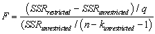
B)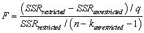
C)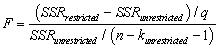
D)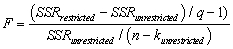
A)
B)
C)
D)
سؤال
سؤال
سؤال
سؤال
سؤال
سؤال
سؤال
سؤال
When testing the null hypothesis that two regression slopes are zero simultaneously,then you cannot reject the null hypothesis at the 5% level,if the ellipse contains the point
A)(-1.96,1.96).
B) .
.
C)(0,0).
D)(1.962,1.962).
A)(-1.96,1.96).
B)
.C)(0,0).
D)(1.962,1.962).
سؤال
All of the following are correct formulae for the homoskedasticity-only F-statistic,with the exception of
A)
B)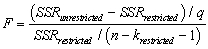
C)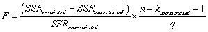
D)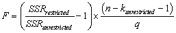
A)
B)
C)
D)
سؤال
All of the following are examples of joint hypotheses on multiple regression coefficients,with the exception of
A)H0 : β1 + β2 = 1
B)H0 : = β1 and β4 = 0
C)H0 : β2 = 0 and β3 = 0
D)H0 : β1 = -β2 and β1 + β2 = 1
A)H0 : β1 + β2 = 1
B)H0 :
= β1 and β4 = 0C)H0 : β2 = 0 and β3 = 0
D)H0 : β1 = -β2 and β1 + β2 = 1
سؤال
سؤال
سؤال
سؤال
سؤال
سؤال
The homoskedasticity-only F-statistic is given by the following formula
A)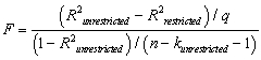
B)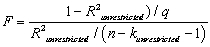
C)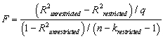
D)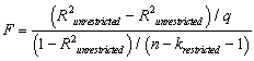
A)
B)
C)
D)
سؤال
سؤال
سؤال
سؤال
The cost of attending your college has once again gone up.Although you have been told that education is investment in human capital,which carries a return of roughly 10% a year,you (and your parents)are not pleased.One of the administrators at your university/college does not make the situation better by telling you that you pay more because the reputation of your institution is better than that of others.To investigate this hypothesis,you collect data randomly for 100 national universities and liberal arts colleges from the 2000-2001 U.S.News and World Report annual rankings.Next you perform the following regression  = 7,311.17 + 3,985.20 × Reputation - 0.20 × Size
(2,058.63)(664.58)(0.13)
+ 8,406.79 × Dpriv - 416.38 × Dlibart - 2,376.51 × Dreligion
(2,154.85)(1,121.92)(1,007.86)
R2=0.72,SER = 3,773.35
where Cost is Tuition,Fees,Room and Board in dollars,Reputation is the index used in U.S.News and World Report (based on a survey of university presidents and chief academic officers),which ranges from 1 ("marginal")to 5 ("distinguished"),Size is the number of undergraduate students,and Dpriv,Dlibart,and Dreligion are binary variables indicating whether the institution is private,a liberal arts college,and has a religious affiliation.The numbers in parentheses are heteroskedasticity-robust standard errors.
(a)Indicate whether or not the coefficients are significantly different from zero.
(b)What is the p-value for the null hypothesis that the coefficient on Size is equal to zero? Based on this,should you eliminate the variable from the regression? Why or why not?
(c)You want to test simultaneously the hypotheses that βsize = 0 and βDilbert = 0.Your regression package returns the F-statistic of 1.23.Can you reject the null hypothesis?
(d)Eliminating the Size and Dlibart variables from your regression,the estimation regression becomes = 5,450.35 + 3,538.84 × Reputation + 10,935.70 × Dpriv - 2,783.31 × Dreligion;
(1,772.35)(590.49)(875.51)(1,180.57)
R2=0.72,SER = 3,792.68
Why do you think that the effect of attending a private institution has increased now?
(e)You give a final attempt to bring the effect of Size back into the equation by forcing the assumption of homoskedasticity onto your estimation.The results are as follows: = 7,311.17 + 3,985.20 × Reputation - 0.20 × Size
(1,985.17)(593.65)(0.07)
+ 8,406.79 × Dpriv - 416.38 × Dlibart - 2,376.51 × Dreligion
(1,423.59)(1,096.49)(989.23)
R2=0.72,SER = 3,682.02
Calculate the t-statistic on the Size coefficient and perform the hypothesis test that its coefficient is zero.Is this test reliable? Explain.
= 7,311.17 + 3,985.20 × Reputation - 0.20 × Size(2,058.63)(664.58)(0.13)
+ 8,406.79 × Dpriv - 416.38 × Dlibart - 2,376.51 × Dreligion
(2,154.85)(1,121.92)(1,007.86)
R2=0.72,SER = 3,773.35
where Cost is Tuition,Fees,Room and Board in dollars,Reputation is the index used in U.S.News and World Report (based on a survey of university presidents and chief academic officers),which ranges from 1 ("marginal")to 5 ("distinguished"),Size is the number of undergraduate students,and Dpriv,Dlibart,and Dreligion are binary variables indicating whether the institution is private,a liberal arts college,and has a religious affiliation.The numbers in parentheses are heteroskedasticity-robust standard errors.
(a)Indicate whether or not the coefficients are significantly different from zero.
(b)What is the p-value for the null hypothesis that the coefficient on Size is equal to zero? Based on this,should you eliminate the variable from the regression? Why or why not?
(c)You want to test simultaneously the hypotheses that βsize = 0 and βDilbert = 0.Your regression package returns the F-statistic of 1.23.Can you reject the null hypothesis?
(d)Eliminating the Size and Dlibart variables from your regression,the estimation regression becomes
= 5,450.35 + 3,538.84 × Reputation + 10,935.70 × Dpriv - 2,783.31 × Dreligion;(1,772.35)(590.49)(875.51)(1,180.57)
R2=0.72,SER = 3,792.68
Why do you think that the effect of attending a private institution has increased now?
(e)You give a final attempt to bring the effect of Size back into the equation by forcing the assumption of homoskedasticity onto your estimation.The results are as follows:
= 7,311.17 + 3,985.20 × Reputation - 0.20 × Size(1,985.17)(593.65)(0.07)
+ 8,406.79 × Dpriv - 416.38 × Dlibart - 2,376.51 × Dreligion
(1,423.59)(1,096.49)(989.23)
R2=0.72,SER = 3,682.02
Calculate the t-statistic on the Size coefficient and perform the hypothesis test that its coefficient is zero.Is this test reliable? Explain.
سؤال
سؤال
At a mathematical level,if the two conditions for omitted variable bias are satisfied,then
A)E(ui X1i,X2i,... ,Xki)≠ 0.
B)there is perfect multicollinearity.
C)large outliers are likely: X1i,X2i,... ,Xki and Yi and have infinite fourth moments.
D)(X1i,X2i,... ,Xki,Yi),i = 1,... ,n are not i.i.d.draws from their joint distribution.
A)E(ui
X1i,X2i,... ,Xki)≠ 0.B)there is perfect multicollinearity.
C)large outliers are likely: X1i,X2i,... ,Xki and Yi and have infinite fourth moments.
D)(X1i,X2i,... ,Xki,Yi),i = 1,... ,n are not i.i.d.draws from their joint distribution.
سؤال
A subsample from the Current Population Survey is taken,on weekly earnings of individuals,their age,and their gender.You have read in the news that women make 70 cents to the $1 that men earn.To test this hypothesis,you first regress earnings on a constant and a binary variable,which takes on a value of 1 for females and is 0 otherwise.The results were:  = 570.70 - 170.72 × Female,R2=0.084,SER = 282.12.
(9.44)(13.52)
(a)Perform a difference in means test and indicate whether or not the difference in the mean salaries is significantly different.Justify your choice of a one-sided or two-sided alternative test.Are these results evidence enough to argue that there is discrimination against females? Why or why not? Is it likely that the errors are normally distributed in this case? If not,does that present a problem to your test?
(b)Test for the significance of the age and gender coefficients.Why do you think that age plays a role in earnings determination?
= 570.70 - 170.72 × Female,R2=0.084,SER = 282.12.(9.44)(13.52)
(a)Perform a difference in means test and indicate whether or not the difference in the mean salaries is significantly different.Justify your choice of a one-sided or two-sided alternative test.Are these results evidence enough to argue that there is discrimination against females? Why or why not? Is it likely that the errors are normally distributed in this case? If not,does that present a problem to your test?
(b)Test for the significance of the age and gender coefficients.Why do you think that age plays a role in earnings determination?
سؤال
The F-statistic with q = 2 restrictions when testing for the restrictions β1 = 0 and β2 = 0 is given by the following formula: 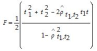 Discuss how this formula can be understood intuitively.
Discuss how this formula can be understood intuitively. سؤال
Consider the following regression output where the dependent variable is testscores and the two explanatory variables are the student-teacher ratio and the percent of English learners:  = 698.9 - 1.10×STR - 0.650×PctEL.You are told that the t-statistic on the student-teacher ratio coefficient is 2.56.The standard error therefore is approximately
A)0.25
B)1.96
C)0.650
D)0.43
= 698.9 - 1.10×STR - 0.650×PctEL.You are told that the t-statistic on the student-teacher ratio coefficient is 2.56.The standard error therefore is approximatelyA)0.25
B)1.96
C)0.650
D)0.43
سؤال
سؤال
سؤال
In the process of collecting weight and height data from 29 female and 81 male students at your university,you also asked the students for the number of siblings they have.Although it was not quite clear to you initially what you would use that variable for,you construct a new theory that suggests that children who have more siblings come from poorer families and will have to share the food on the table.Although a friend tells you that this theory does not pass the "straight-face" test,you decide to hypothesize that peers with many siblings will weigh less,on average,for a given height.In addition,you believe that the muscle/fat tissue composition of male bodies suggests that females will weigh less,on average,for a given height.To test these theories,you perform the following regression:  = -229.92 - 6.52 × Female + 0.51 × Sibs+ 5.58 × Height,
(44.01)(5.52)(2.25)(0.62)
R2=0.50,SER = 21.08
where Studentw is in pounds,Height is in inches,Female takes a value of 1 for females and is 0 otherwise,Sibs is the number of siblings (heteroskedasticity-robust standard errors in parentheses).
(a)Carrying out hypotheses tests using the relevant t-statistics to test your two claims separately,is there strong evidence in favor of your hypotheses? Is it appropriate to use two separate tests in this situation?
(b)You also perform an F-test on the joint hypothesis that the two coefficients for females and siblings are zero.The calculated F-statistic is 0.84.Find the critical value from the F-table.Can you reject the null hypothesis? Is it possible that one of the two parameters is zero in the population,but not the other?
(c)You are now a bit worried that the entire regression does not make sense and therefore also test for the height coefficient to be zero.The resulting F-statistic is 57.25.Does that prove that there is a relationship between weight and height?
= -229.92 - 6.52 × Female + 0.51 × Sibs+ 5.58 × Height,(44.01)(5.52)(2.25)(0.62)
R2=0.50,SER = 21.08
where Studentw is in pounds,Height is in inches,Female takes a value of 1 for females and is 0 otherwise,Sibs is the number of siblings (heteroskedasticity-robust standard errors in parentheses).
(a)Carrying out hypotheses tests using the relevant t-statistics to test your two claims separately,is there strong evidence in favor of your hypotheses? Is it appropriate to use two separate tests in this situation?
(b)You also perform an F-test on the joint hypothesis that the two coefficients for females and siblings are zero.The calculated F-statistic is 0.84.Find the critical value from the F-table.Can you reject the null hypothesis? Is it possible that one of the two parameters is zero in the population,but not the other?
(c)You are now a bit worried that the entire regression does not make sense and therefore also test for the height coefficient to be zero.The resulting F-statistic is 57.25.Does that prove that there is a relationship between weight and height?
سؤال
سؤال
In the multiple regression model with two explanatory variables
Yi = β0 + β1X1i + β2X2i + ui
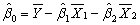
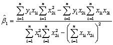
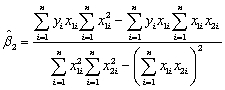
the OLS estimators for the three parameters are as follows (small letters refer to deviations from means as in zi = Zi - ):
): 
 You have collected data for 104 countries of the world from the Penn World Tables and want to estimate the effect of the population growth rate (X1i)and the saving rate (X2i)(average investment share of GDP from 1980 to 1990)on GDP per worker (relative to the U.S. )in 1990.The various sums needed to calculate the OLS estimates are given below:
  = 33.33;
  = 2.025;
  =17.313
  = 8.3103;
  = .0122;
  = 0.6422
  = - 0.2304;
  = 1.5676;
  = -0.0520
The heteroskedasticity-robust standard errors of the two slope coefficients are 1.99 (for population growth)and 0.23 (for the saving rate).Calculate the 95% confidence interval for both coefficients.How many standard deviations are the coefficients away from zero?
Yi = β0 + β1X1i + β2X2i + ui
the OLS estimators for the three parameters are as follows (small letters refer to deviations from means as in zi = Zi -
): You have collected data for 104 countries of the world from the Penn World Tables and want to estimate the effect of the population growth rate (X1i)and the saving rate (X2i)(average investment share of GDP from 1980 to 1990)on GDP per worker (relative to the U.S. )in 1990.The various sums needed to calculate the OLS estimates are given below: = 33.33; = 2.025; =17.313 = 8.3103; = .0122; = 0.6422 = - 0.2304; = 1.5676; = -0.0520The heteroskedasticity-robust standard errors of the two slope coefficients are 1.99 (for population growth)and 0.23 (for the saving rate).Calculate the 95% confidence interval for both coefficients.How many standard deviations are the coefficients away from zero?
سؤال
The administration of your university/college is thinking about implementing a policy of coed floors only in dormitories.Currently there are only single gender floors.One reason behind such a policy might be to generate an atmosphere of better "understanding" between the sexes.The Dean of Students (DoS)has decided to investigate if such a behavior results in more "togetherness" by attempting to find the determinants of the gender composition at the dinner table in your main dining hall,and in that of a neighboring university,which only allows for coed floors in their dorms.The survey includes 176 students,63 from your university/college,and 113 from a neighboring institution.
The Dean's first problem is how to define gender composition.To begin with,the survey excludes single persons' tables,since the study is to focus on group behavior.The Dean also eliminates sports teams from the analysis,since a large number of single-gender students will sit at the same table.Finally,the Dean decides to only analyze tables with three or more students,since she worries about "couples" distorting the results.The Dean finally settles for the following specification of the dependent variable:
GenderComp = Where "
  " stands for absolute value of Z.The variable can take on values from zero to fifty.
After considering various explanatory variables,the Dean settles for an initial list of eight,and estimates the following relationship,using heteroskedasticity-robust standard errors (this Dean obviously has taken an econometrics course earlier in her career and/or has an able research assistant): = 30.90 - 3.78 × Size - 8.81 × DCoed + 2.28 × DFemme +2.06 × DRoommate
(7.73)(0.63)(2.66)(2.42)(2.39)
- 0.17 × DAthlete + 1.49 × DCons - 0.81 SAT + 1.74 × SibOther,R2=0.24,SER = 15.50
(3.23)(1.10)(1.20)(1.43)
where Size is the number of persons at the table minus 3;DCoed is a binary variable,which takes on the value of 1 if you live on a coed floor;DFemme is a binary variable,which is 1 for females and zero otherwise;DRoommate is a binary variable which equals 1 if the person at the table has a roommate and is zero otherwise;DAthlete is a binary variable which is 1 if the person at the table is a member of an athletic varsity team;DCons is a variable which measures the political tendency of the person at the table on a seven-point scale,ranging from 1 being "liberal" to 7 being "conservative";SAT is the SAT score of the person at the table measured on a seven-point scale,ranging from 1 for the category "900-1000" to 7 for the category "1510 and above";and increasing by one for 100 point increases;and SibOther is the number of siblings from the opposite gender in the family the person at the table grew up with.
(a)Indicate which of the coefficients are statistically significant.
(b)Based on the above results,the Dean decides to specify a more parsimonious form by eliminating the least significant variables.Using the F-statistic for the null hypothesis that there is no relationship between the gender composition at the table and DFemme,DRoommate,DAthlete,and SAT,the regression package returns a value of 1.10.What are the degrees of freedom for the statistic? Look up the 1% and 5% critical values from the F- table and make a decision about the exclusion of these variables based on the critical values.
(c)The Dean decides to estimate the following specification next: = 29.07 - 3.80 × Size - 9.75 × DCoed + 1.50 × DCons + 1.97 × SibOther,
(3.75)(0.62)(1.04)(1.04)(1.44)
R2=0.22 SER = 15.44
Calculate the t-statistics for the coefficients and discuss whether or not the Dean should attempt to simplify the specification further.Based on the results,what might some of the comments be that she will write up for the other senior administrators of your college? What are some of the potential flaws in her analysis? What other variables do you think she should have considered as explanatory factors?
The Dean's first problem is how to define gender composition.To begin with,the survey excludes single persons' tables,since the study is to focus on group behavior.The Dean also eliminates sports teams from the analysis,since a large number of single-gender students will sit at the same table.Finally,the Dean decides to only analyze tables with three or more students,since she worries about "couples" distorting the results.The Dean finally settles for the following specification of the dependent variable:
GenderComp =
Where " " stands for absolute value of Z.The variable can take on values from zero to fifty.After considering various explanatory variables,the Dean settles for an initial list of eight,and estimates the following relationship,using heteroskedasticity-robust standard errors (this Dean obviously has taken an econometrics course earlier in her career and/or has an able research assistant):
= 30.90 - 3.78 × Size - 8.81 × DCoed + 2.28 × DFemme +2.06 × DRoommate(7.73)(0.63)(2.66)(2.42)(2.39)
- 0.17 × DAthlete + 1.49 × DCons - 0.81 SAT + 1.74 × SibOther,R2=0.24,SER = 15.50
(3.23)(1.10)(1.20)(1.43)
where Size is the number of persons at the table minus 3;DCoed is a binary variable,which takes on the value of 1 if you live on a coed floor;DFemme is a binary variable,which is 1 for females and zero otherwise;DRoommate is a binary variable which equals 1 if the person at the table has a roommate and is zero otherwise;DAthlete is a binary variable which is 1 if the person at the table is a member of an athletic varsity team;DCons is a variable which measures the political tendency of the person at the table on a seven-point scale,ranging from 1 being "liberal" to 7 being "conservative";SAT is the SAT score of the person at the table measured on a seven-point scale,ranging from 1 for the category "900-1000" to 7 for the category "1510 and above";and increasing by one for 100 point increases;and SibOther is the number of siblings from the opposite gender in the family the person at the table grew up with.
(a)Indicate which of the coefficients are statistically significant.
(b)Based on the above results,the Dean decides to specify a more parsimonious form by eliminating the least significant variables.Using the F-statistic for the null hypothesis that there is no relationship between the gender composition at the table and DFemme,DRoommate,DAthlete,and SAT,the regression package returns a value of 1.10.What are the degrees of freedom for the statistic? Look up the 1% and 5% critical values from the F- table and make a decision about the exclusion of these variables based on the critical values.
(c)The Dean decides to estimate the following specification next:
= 29.07 - 3.80 × Size - 9.75 × DCoed + 1.50 × DCons + 1.97 × SibOther,(3.75)(0.62)(1.04)(1.04)(1.44)
R2=0.22 SER = 15.44
Calculate the t-statistics for the coefficients and discuss whether or not the Dean should attempt to simplify the specification further.Based on the results,what might some of the comments be that she will write up for the other senior administrators of your college? What are some of the potential flaws in her analysis? What other variables do you think she should have considered as explanatory factors?
سؤال
سؤال
You have estimated the relationship between testscores and the student-teacher ratio under the assumption of homoskedasticity of the error terms.The regression output is as follows:  = 698.9 - 2.28 × STR,and the standard error on the slope is 0.48.The homoskedasticity-only "overall" regression F- statistic for the hypothesis that the Regression R2 is zero is approximately
A)0.96
B)1.96
C)22.56
D)4.75
= 698.9 - 2.28 × STR,and the standard error on the slope is 0.48.The homoskedasticity-only "overall" regression F- statistic for the hypothesis that the Regression R2 is zero is approximatelyA)0.96
B)1.96
C)22.56
D)4.75
سؤال
You have collected data from Major League Baseball (MLB)to find the determinants of winning.You have a general idea that both good pitching and strong hitting are needed to do well.However,you do not know how much each of these contributes separately.To investigate this problem,you collect data for all MLB during 1999 season.Your strategy is to first regress the winning percentage on pitching quality ("Team ERA"),second to regress the same variable on some measure of hitting ("OPS - On-base Plus Slugging percentage"),and third to regress the winning percentage on both.
Summary of the Distribution of Winning Percentage,On Base plus Slugging Percentage,
and Team Earned Run Average for MLB in 1999
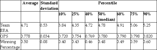 The results are as follows:
  = 0.94 - 0.100 × teamera,R2 = 0.49,SER = 0.06.
(0.08)(0.017) = -0.68 + 1.513 × ops,R2=0.45,SER = 0.06.
(0.17)(0.221) = -0.19 - 0.099 × teamera + 1.490 × ops,R2=0.92,SER = 0.02.
(0.08)(0.008)(0.126)
(a)Use the t-statistic to test for the statistical significance of the coefficient.
(b)There are 30 teams in MLB.Does the small sample size worry you here when testing for significance?
Summary of the Distribution of Winning Percentage,On Base plus Slugging Percentage,
and Team Earned Run Average for MLB in 1999
The results are as follows: = 0.94 - 0.100 × teamera,R2 = 0.49,SER = 0.06.(0.08)(0.017)
= -0.68 + 1.513 × ops,R2=0.45,SER = 0.06.(0.17)(0.221)
= -0.19 - 0.099 × teamera + 1.490 × ops,R2=0.92,SER = 0.02.(0.08)(0.008)(0.126)
(a)Use the t-statistic to test for the statistical significance of the coefficient.
(b)There are 30 teams in MLB.Does the small sample size worry you here when testing for significance?
سؤال
سؤال
Attendance at sports events depends on various factors.Teams typically do not change ticket prices from game to game to attract more spectators to less attractive games.However,there are other marketing tools used,such as fireworks,free hats,etc. ,for this purpose.You work as a consultant for a sports team,the Los Angeles Dodgers,to help them forecast attendance,so that they can potentially devise strategies for price discrimination.After collecting data over two years for every one of the 162 home games of the 2000 and 2001 season,you run the following regression:  = 15,005 + 201 × Temperat + 465 × DodgNetWin + 82 × OppNetWin
(8,770)(121)(169)(26)
+ 9647 × DFSaSu + 1328 × Drain + 1609 × D150m + 271 × DDiv - 978 × D2001;
(1505)(3355)(1819)(1,184)(1,143)
R2=0.416,SER = 6983
where Attend is announced stadium attendance,Temperat it the average temperature on game day,DodgNetWin are the net wins of the Dodgers before the game (wins-losses),OppNetWin is the opposing team's net wins at the end of the previous season,and DFSaSu,Drain,D150m,Ddiv,and D2001 are binary variables,taking a value of 1 if the game was played on a weekend,it rained during that day,the opposing team was within a 150 mile radius,the opposing team plays in the same division as the Dodgers,and the game was played during 2001,respectively.Numbers in parentheses are heteroskedasticity- robust standard errors.
(a)Are the slope coefficients statistically significant?
(b)To test whether the effect of the last four binary variables is significant,you have your regression program calculate the relevant F-statistic,which is 0.295.What is the critical value? What is your decision about excluding these variables?
= 15,005 + 201 × Temperat + 465 × DodgNetWin + 82 × OppNetWin(8,770)(121)(169)(26)
+ 9647 × DFSaSu + 1328 × Drain + 1609 × D150m + 271 × DDiv - 978 × D2001;
(1505)(3355)(1819)(1,184)(1,143)
R2=0.416,SER = 6983
where Attend is announced stadium attendance,Temperat it the average temperature on game day,DodgNetWin are the net wins of the Dodgers before the game (wins-losses),OppNetWin is the opposing team's net wins at the end of the previous season,and DFSaSu,Drain,D150m,Ddiv,and D2001 are binary variables,taking a value of 1 if the game was played on a weekend,it rained during that day,the opposing team was within a 150 mile radius,the opposing team plays in the same division as the Dodgers,and the game was played during 2001,respectively.Numbers in parentheses are heteroskedasticity- robust standard errors.
(a)Are the slope coefficients statistically significant?
(b)To test whether the effect of the last four binary variables is significant,you have your regression program calculate the relevant F-statistic,which is 0.295.What is the critical value? What is your decision about excluding these variables?
سؤال
All of the following are true,with the exception of one condition:
A)a high R2 or does not mean that the regressors are a true cause of the dependent variable.
B)a high R2 or does not mean that there is no omitted variable bias.
C)a high R2 or always means that an added variable is statistically significant.
D)a high R2 or does not necessarily mean that you have the most appropriate set of regressors.
A)a high R2 or
does not mean that the regressors are a true cause of the dependent variable.B)a high R2 or
does not mean that there is no omitted variable bias.C)a high R2 or
always means that an added variable is statistically significant.D)a high R2 or
does not necessarily mean that you have the most appropriate set of regressors. سؤال
The Solow growth model suggests that countries with identical saving rates and population growth rates should converge to the same per capita income level.This result has been extended to include investment in human capital (education)as well as investment in physical capital.This hypothesis is referred to as the "conditional convergence hypothesis," since the convergence is dependent on countries obtaining the same values in the driving variables.To test the hypothesis,you collect data from the Penn World Tables on the average annual growth rate of GDP per worker (g6090)for the 1960-1990 sample period,and regress it on the (i)initial starting level of GD-P per worker relative to the United States in 1960 (RelProd60), (ii)average population growth rate of the country (n), (iii)average investment share of GDP from 1960 to 1990 (SK - remember investment equals savings),and (iv)educational attainment in years for 1985 (Educ).The results for close to 100 countries is as follows (numbers in parentheses are for heteroskedasticity-robust standard errors):  = 0.004 - 0.172 × n + 0.133 × SK + 0.002 × Educ - 0.044 × RelProd60,
(0.007)(0.209)(0.015)(0.001)(0.008)
R2=0.537,SER = 0.011
(a)Is the coefficient on this variable significantly different from zero at the 5% level? At the 1% level?
(b)Test for the significance of the other slope coefficients.Should you use a one-sided alternative hypothesis or a two-sided test? Will the decision for one or the other influence the decision about the significance of the parameters? Should you always eliminate variables which carry insignificant coefficients?
= 0.004 - 0.172 × n + 0.133 × SK + 0.002 × Educ - 0.044 × RelProd60,(0.007)(0.209)(0.015)(0.001)(0.008)
R2=0.537,SER = 0.011
(a)Is the coefficient on this variable significantly different from zero at the 5% level? At the 1% level?
(b)Test for the significance of the other slope coefficients.Should you use a one-sided alternative hypothesis or a two-sided test? Will the decision for one or the other influence the decision about the significance of the parameters? Should you always eliminate variables which carry insignificant coefficients?
سؤال
You have collected data for 104 countries to address the difficult questions of the determinants for differences in the standard of living among the countries of the world.You recall from your macroeconomics lectures that the neoclassical growth model suggests that output per worker (per capita income)levels are determined by,among others,the saving rate and population growth rate.To test the predictions of this growth model,you run the following regression:  = 0.339 - 12.894 × n + 1.397 × SK,R2=0.621,SER = 0.177
(0.068)(3.177)(0.229)
where RelPersInc is GDP per worker relative to the United States,n is the average population growth rate,1980-1990,and SK is the average investment share of GDP from 1960 to 1990 (remember investment equals saving).Numbers in parentheses are for heteroskedasticity-robust standard errors.
(a)Calculate the t-statistics and test whether or not each of the population parameters are significantly different from zero.
(b)The overall F-statistic for the regression is 79.11.What is the critical value at the 5% and 1% level? What is your decision on the null hypothesis?
(c)You remember that human capital in addition to physical capital also plays a role in determining the standard of living of a country.You therefore collect additional data on the average educational attainment in years for 1985,and add this variable (Educ)to the above regression.This results in the modified regression output: = 0.046 - 5.869 × n + 0.738 × SK + 0.055 × Educ,R2=0.775,SER = 0.1377
(0.079)(2.238)(0.294)(0.010)
How has the inclusion of Educ affected your previous results?
(d)Upon checking the regression output,you realize that there are only 86 observations,since data for Educ is not available for all 104 countries in your sample.Do you have to modify some of your statements in (d)?
= 0.339 - 12.894 × n + 1.397 × SK,R2=0.621,SER = 0.177(0.068)(3.177)(0.229)
where RelPersInc is GDP per worker relative to the United States,n is the average population growth rate,1980-1990,and SK is the average investment share of GDP from 1960 to 1990 (remember investment equals saving).Numbers in parentheses are for heteroskedasticity-robust standard errors.
(a)Calculate the t-statistics and test whether or not each of the population parameters are significantly different from zero.
(b)The overall F-statistic for the regression is 79.11.What is the critical value at the 5% and 1% level? What is your decision on the null hypothesis?
(c)You remember that human capital in addition to physical capital also plays a role in determining the standard of living of a country.You therefore collect additional data on the average educational attainment in years for 1985,and add this variable (Educ)to the above regression.This results in the modified regression output:
= 0.046 - 5.869 × n + 0.738 × SK + 0.055 × Educ,R2=0.775,SER = 0.1377(0.079)(2.238)(0.294)(0.010)
How has the inclusion of Educ affected your previous results?
(d)Upon checking the regression output,you realize that there are only 86 observations,since data for Educ is not available for all 104 countries in your sample.Do you have to modify some of your statements in (d)?
سؤال
Consider the following regression using the California School data set from your textbook.  = 681.44 - 0.61LchPct
n=420,R2=0.75,SER=9.45
where TestScore is the test score and LchPct is the percent of students eligible for subsidized lunch (average = 44.7,max = 100,min = 0).
a.What is the effect of a 20 percentage point increase in the student eligible for subsidized lunch?
b.Your textbook started with the following regression in Chapter 4: = 698.9 - 2.28STR
n=420,R2=0.051,SER=18.58
where STR is the student teacher ratio.
Your textbook tells you that in the multiple regression framework considered,the percentage of students eligible for subsidized lunch is a control variable,while the student teacher ratio is the variable of interest.Given that the regression R2 is so much higher for the first equation than for the second equation,shouldn't the role of the two variables be reversed? That is,shouldn't the student teacher ratio be the control variable while the percent of students eligible for subsidized lunch be the variable of interest?
= 681.44 - 0.61LchPctn=420,R2=0.75,SER=9.45
where TestScore is the test score and LchPct is the percent of students eligible for subsidized lunch (average = 44.7,max = 100,min = 0).
a.What is the effect of a 20 percentage point increase in the student eligible for subsidized lunch?
b.Your textbook started with the following regression in Chapter 4:
= 698.9 - 2.28STRn=420,R2=0.051,SER=18.58
where STR is the student teacher ratio.
Your textbook tells you that in the multiple regression framework considered,the percentage of students eligible for subsidized lunch is a control variable,while the student teacher ratio is the variable of interest.Given that the regression R2 is so much higher for the first equation than for the second equation,shouldn't the role of the two variables be reversed? That is,shouldn't the student teacher ratio be the control variable while the percent of students eligible for subsidized lunch be the variable of interest?
سؤال
The homoskedasticity only F-statistic is given by the formula 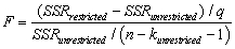 where SSRrestricted is the sum of squared residuals from the restricted regression,SSRunrestricted is the sum of squared residuals from the unrestricted regression,q is the number of restrictions under the null hypothesis,and kunrestricted is the number of regressors in the unrestricted regression.Prove that this formula is the same as the following formula based on the regression R2 of the restricted and unrestricted regression:
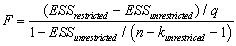
where SSRrestricted is the sum of squared residuals from the restricted regression,SSRunrestricted is the sum of squared residuals from the unrestricted regression,q is the number of restrictions under the null hypothesis,and kunrestricted is the number of regressors in the unrestricted regression.Prove that this formula is the same as the following formula based on the regression R2 of the restricted and unrestricted regression: سؤال
سؤال
سؤال
Prove that 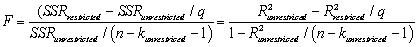
سؤال
To calculate the homoskedasticity-only overall regression F-statistic,you need to compare the SSRrestricted with the SSRunrestricted.Consider the following output from a regression package,which reproduces the regression results of testscores on the student-teacher ratio,the percent of English learners,and the expenditures per student from your textbook:
Dependent Variable: TESTSCR
Method: Least Squares
Date: 07/30/06 Time: 17:55
Sample: 1 420
Included observations: 420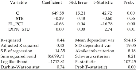 Sum of squared resid corresponds to SSRunrestricted.How are you going to find SSRrestricted?
Dependent Variable: TESTSCR
Method: Least Squares
Date: 07/30/06 Time: 17:55
Sample: 1 420
Included observations: 420
Sum of squared resid corresponds to SSRunrestricted.How are you going to find SSRrestricted? سؤال
سؤال
Consider the following regression output for an unrestricted and a restricted model.
Unrestricted model:
Dependent Variable: TESTSCR
Method: Least Squares
Date: 07/31/06 Time: 17:35
Sample: 1 420
Included observations: 420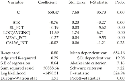 Restricted model:
Dependent Variable: TESTSCR
Method: Least Squares
Date: 07/31/06 Time: 17:37
Sample: 1 420
Included observations: 420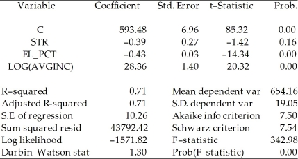 Calculate the homoskedasticity only F-statistic and determine whether the null hypothesis can be rejected at the 5% significance level.
Unrestricted model:
Dependent Variable: TESTSCR
Method: Least Squares
Date: 07/31/06 Time: 17:35
Sample: 1 420
Included observations: 420
Restricted model:Dependent Variable: TESTSCR
Method: Least Squares
Date: 07/31/06 Time: 17:37
Sample: 1 420
Included observations: 420
Calculate the homoskedasticity only F-statistic and determine whether the null hypothesis can be rejected at the 5% significance level. سؤال
Consider the following Cobb-Douglas production function Yi = AK  L
L 
 (where Y is output,A is the level of technology,K is the capital stock,and L is the labor force),which has been linearized here (by using logarithms)to look as follows:
yi = + β1ki + β2li + ui
Assuming that the errors are heteroskedastic,you want to test for constant returns to scale.Using a t-statistic and "Approach #2," how would you proceed.
L (where Y is output,A is the level of technology,K is the capital stock,and L is the labor force),which has been linearized here (by using logarithms)to look as follows:yi =
+ β1ki + β2li + uiAssuming that the errors are heteroskedastic,you want to test for constant returns to scale.Using a t-statistic and "Approach #2," how would you proceed.
سؤال
Your textbook has emphasized that testing two hypothesis sequentially is not the same as testing them simultaneously.Consider the following confidence set below,where you are testing the hypothesis that H0 : β5 = 0,β6 = 0.  Your statistical package has also generated a dotted area,which corresponds to drawing two confidence intervals for the respective coefficients.For each case where the ellipse does not coincide in area with the corresponding rectangle,indicate what your decision would be if you relied on the two confidence intervals vs.the ellipse generated by the F-statistic.
Your statistical package has also generated a dotted area,which corresponds to drawing two confidence intervals for the respective coefficients.For each case where the ellipse does not coincide in area with the corresponding rectangle,indicate what your decision would be if you relied on the two confidence intervals vs.the ellipse generated by the F-statistic. سؤال
سؤال
Consider the following two models to explain testscores.
Model 1:
Dependent Variable: TESTSCR
Method: Least Squares
Date: 07/31/06 Time: 17:52
Sample: 1 420
Included observations: 420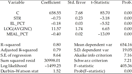 Model 2:
Dependent Variable: TESTSCR
Method: Least Squares
Date: 07/31/06 Time: 17:56
Sample: 1 420
Included observations: 420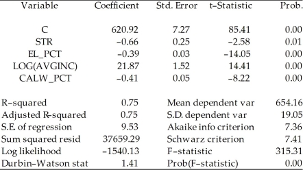 Explain why you cannot use the F-test in this situation to discriminate between Model 1 and Model 2.
Model 1:
Dependent Variable: TESTSCR
Method: Least Squares
Date: 07/31/06 Time: 17:52
Sample: 1 420
Included observations: 420
Model 2:Dependent Variable: TESTSCR
Method: Least Squares
Date: 07/31/06 Time: 17:56
Sample: 1 420
Included observations: 420
Explain why you cannot use the F-test in this situation to discriminate between Model 1 and Model 2. سؤال
Females,on average,are shorter and weigh less than males.One of your friends,who is a pre-med student,tells you that in addition,females will weigh less for a given height.To test this hypothesis,you collect height and weight of 29 female and 81 male students at your university.A regression of the weight on a constant,height,and a binary variable,which takes a value of one for females and is zero otherwise,yields the following result:  = -229.21 - 6.36 × Female + 5.58 × Height,R2=0.50,SER = 20.99
(43.39)(5.74)(0.62)
where Studentw is weight measured in pounds and Height is measured in inches (heteroskedasticity-robust standard errors in parentheses).
Calculate t-statistics and carry out the hypothesis test that females weigh the same as males,on average,for a given height,using a 10% significance level.What is the alternative hypothesis? What is the p-value? What critical value did you use?
= -229.21 - 6.36 × Female + 5.58 × Height,R2=0.50,SER = 20.99(43.39)(5.74)(0.62)
where Studentw is weight measured in pounds and Height is measured in inches (heteroskedasticity-robust standard errors in parentheses).
Calculate t-statistics and carry out the hypothesis test that females weigh the same as males,on average,for a given height,using a 10% significance level.What is the alternative hypothesis? What is the p-value? What critical value did you use?
سؤال
Give an intuitive explanation for 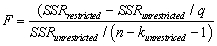 .Name conditions under which the F-statistic is large and hence rejects the null hypothesis.
.Name conditions under which the F-statistic is large and hence rejects the null hypothesis. سؤال
سؤال
سؤال
Using the 420 observations of the California School data set from your textbook,you estimate the following relationship:  = 681.44 - 0.61LchPct
n=420,R2=0.75,SER=9.45
where TestScore is the test score and LchPct is the percent of students eligible for subsidized lunch (average = 44.7,max = 100,min = 0).
a.Interpret the regression result.
b.In your interpretation of the slope coefficient in (a)above,does it matter if you start your explanation with "for every x percent increase" rather than "for every x percentage point increase"?
c.The "overall" regression F-statistic is 1149.57.What are the degrees of freedom for this statistic?
d.Find the critical value of the F-statistic at the 1% significance level.Test the null hypothesis that the regression R2= 0.
e.The above equation was estimated using heteroskedasticity robust standard errors.What is the standard error for the slope coefficient?
= 681.44 - 0.61LchPctn=420,R2=0.75,SER=9.45
where TestScore is the test score and LchPct is the percent of students eligible for subsidized lunch (average = 44.7,max = 100,min = 0).
a.Interpret the regression result.
b.In your interpretation of the slope coefficient in (a)above,does it matter if you start your explanation with "for every x percent increase" rather than "for every x percentage point increase"?
c.The "overall" regression F-statistic is 1149.57.What are the degrees of freedom for this statistic?
d.Find the critical value of the F-statistic at the 1% significance level.Test the null hypothesis that the regression R2= 0.
e.The above equation was estimated using heteroskedasticity robust standard errors.What is the standard error for the slope coefficient?
سؤال
Consider the regression model Yi = β0 + β1X1i + β2X2i+ β3X3i + ui.Use "Approach #2" from Section 7.3 to transform the regression so that you can use a t-statistic to test:
β1 =
β1 =
سؤال
Consider the regression output from the following unrestricted model:
Unrestricted model:
Dependent Variable: TESTSCR
Method: Least Squares
Date: 07/31/06 Time: 17:35
Sample: 1 420
Included observations: 420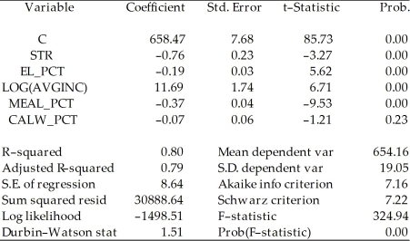 To test for the null hypothesis that neither coefficient on the percent eligible for subsidized lunch nor the coefficient on the percent on public income assistance is statistically significant,you have your statistical package plot the confidence set.Interpret the graph below and explain what it tells you about the null hypothesis.
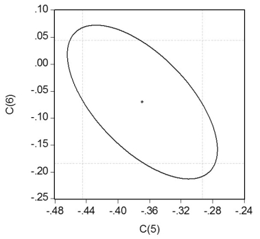
Unrestricted model:
Dependent Variable: TESTSCR
Method: Least Squares
Date: 07/31/06 Time: 17:35
Sample: 1 420
Included observations: 420
To test for the null hypothesis that neither coefficient on the percent eligible for subsidized lunch nor the coefficient on the percent on public income assistance is statistically significant,you have your statistical package plot the confidence set.Interpret the graph below and explain what it tells you about the null hypothesis. سؤال
You are presented with the following output from a regression package,which reproduces the regression results of testscores on the student-teacher ratio from your textbook
Dependent Variable: TESTSCR
Method: Least Squares
Date: 07/30/06 Time: 17:44
Sample: 1 420
Included observations: 420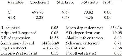 Std.Error are homoskedasticity only standard errors.
a)What is the relationship between the t-statistic on the student-teacher ratio coefficient and the F-statistic?
b)Next,two explanatory variables,the percent of English learners (EL_PCT)and expenditures per student (EXPN_STU)are added.The output is listed as below.What is the relationship between the three t-statistics for the slopes and the homoskedasticity-only F-statistic now?
Dependent Variable: TESTSCR
Method: Least Squares
Date: 07/30/06 Time: 17:55
Sample: 1 420
Included observations: 420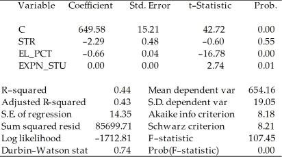
Dependent Variable: TESTSCR
Method: Least Squares
Date: 07/30/06 Time: 17:44
Sample: 1 420
Included observations: 420
Std.Error are homoskedasticity only standard errors.a)What is the relationship between the t-statistic on the student-teacher ratio coefficient and the F-statistic?
b)Next,two explanatory variables,the percent of English learners (EL_PCT)and expenditures per student (EXPN_STU)are added.The output is listed as below.What is the relationship between the three t-statistics for the slopes and the homoskedasticity-only F-statistic now?
Dependent Variable: TESTSCR
Method: Least Squares
Date: 07/30/06 Time: 17:55
Sample: 1 420
Included observations: 420
سؤال
Analyzing a regression using data from a sub-sample of the Current Population Survey with about 4,000 observations,you realize that the regression R2,and the adjusted R2,  2,are almost identical.Why is that the case? In your textbook,you were told that the regression R2 will almost always increase when you add an explanatory variable,but that the adjusted measure does not have to increase with such an addition.Can this still be true?
2,are almost identical.Why is that the case? In your textbook,you were told that the regression R2 will almost always increase when you add an explanatory variable,but that the adjusted measure does not have to increase with such an addition.Can this still be true? سؤال
You have estimated the following regression to explain hourly wages,using a sample of 250 individuals:  = -2.44 - 1.57 × DFemme + 0.27 × DMarried + 0.59 × Educ + 0.04 × Exper - 0.60 × DNonwhite
(1.29)(0.33)(0.36)(0.09)(0.01)(0.49)
+ 0.13 × NCentral - 0.11 × South
(0.59)(0.58)
R2 = 0.36,SER = 2.74,n = 250
Test the null hypothesis that the coefficients on DMarried,DNonwhite,and the two regional variables,NCentral and South are zero.The F-statistic for the null hypothesis βmarried = βnonwhite = βnonwhite = βncentral = βsouth = 0 is 0.61.Do you reject the null hypothesis?
= -2.44 - 1.57 × DFemme + 0.27 × DMarried + 0.59 × Educ + 0.04 × Exper - 0.60 × DNonwhite(1.29)(0.33)(0.36)(0.09)(0.01)(0.49)
+ 0.13 × NCentral - 0.11 × South
(0.59)(0.58)
R2 = 0.36,SER = 2.74,n = 250
Test the null hypothesis that the coefficients on DMarried,DNonwhite,and the two regional variables,NCentral and South are zero.The F-statistic for the null hypothesis βmarried = βnonwhite = βnonwhite = βncentral = βsouth = 0 is 0.61.Do you reject the null hypothesis?
سؤال
سؤال
Using the California School data set from your textbook,you decide to run a regression of the average reading score (ScrRead)on the average mathematics score (ScrMaths).The result is as follows,where the numbers in parenthesis are homoskedasticity only standard errors:  = 8.47 + 0.9895×ScrMaths
(13.20)(0.0202)
N = 420,R2 = 0.85,SER = 7.8
You believe that the average mathematics score is an unbiased predictor of the average reading score.Consider the above regression to be the unrestricted from which you would calculate SSRUnrestricted .How would you find the SSRRestricted? How many restrictions would have to impose?
= 8.47 + 0.9895×ScrMaths(13.20)(0.0202)
N = 420,R2 = 0.85,SER = 7.8
You believe that the average mathematics score is an unbiased predictor of the average reading score.Consider the above regression to be the unrestricted from which you would calculate SSRUnrestricted .How would you find the SSRRestricted? How many restrictions would have to impose?
سؤال
Looking at formula (7.13)in your textbook for the homoskedasticity-only F-statistic, 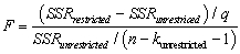 give three conditions under which,ceteris paribus,you would find a large value,and hence would be likely to reject the null hypothesis.
give three conditions under which,ceteris paribus,you would find a large value,and hence would be likely to reject the null hypothesis.
فتح الحزمة
قم بالتسجيل لفتح البطاقات في هذه المجموعة!
Unlock Deck
Unlock Deck
1/65
العب
ملء الشاشة (f)
Deck 7: Hypothesis Tests and Confidence Intervals in Multiple Regression
1
The homoskedasticity-only F-statistic is given by the following formula
A)
B)
C)
D)
A)
B)
C)
D)
A
2
If you reject a joint null hypothesis using the F-test in a multiple hypothesis setting,then
A)a series of t-tests may or may not give you the same conclusion.
B)the regression is always significant.
C)all of the hypotheses are always simultaneously rejected.
D)the F-statistic must be negative.
A)a series of t-tests may or may not give you the same conclusion.
B)the regression is always significant.
C)all of the hypotheses are always simultaneously rejected.
D)the F-statistic must be negative.
A
3
If you wanted to test,using a 5% significance level,whether or not a specific slope coefficient is equal to one,then you should
A)subtract 1 from the estimated coefficient,divide the difference by the standard error,and check if the resulting ratio is larger than 1.96.
B)add and subtract 1.96 from the slope and check if that interval includes 1.
C)see if the slope coefficient is between 0.95 and 1.05.
D)check if the adjusted R2 is close to 1.
A
4
The following linear hypothesis can be tested using the F-test with the exception of
A)β2 = 1 and β3= β4/β5.
B)β2 =0.
C)β1 + β2 = 1 and β3 = -2β4.
D)β0 = β1 and β1 = 0.
A)β2 = 1 and β3= β4/β5.
B)β2 =0.
C)β1 + β2 = 1 and β3 = -2β4.
D)β0 = β1 and β1 = 0.
فتح الحزمة
افتح القفل للوصول البطاقات البالغ عددها 65 في هذه المجموعة.
فتح الحزمة
k this deck
5
When there are two coefficients,the resulting confidence sets are
A)rectangles.
B)ellipses.
C)squares.
D)trapezoids.
A)rectangles.
B)ellipses.
C)squares.
D)trapezoids.
فتح الحزمة
افتح القفل للوصول البطاقات البالغ عددها 65 في هذه المجموعة.
فتح الحزمة
k this deck
6
The overall regression F-statistic tests the null hypothesis that
A)all slope coefficients are zero.
B)all slope coefficients and the intercept are zero.
C)the intercept in the regression and at least one,but not all,of the slope coefficients is zero.
D)the slope coefficient of the variable of interest is zero,but that the other slope coefficients are not.
A)all slope coefficients are zero.
B)all slope coefficients and the intercept are zero.
C)the intercept in the regression and at least one,but not all,of the slope coefficients is zero.
D)the slope coefficient of the variable of interest is zero,but that the other slope coefficients are not.
فتح الحزمة
افتح القفل للوصول البطاقات البالغ عددها 65 في هذه المجموعة.
فتح الحزمة
k this deck
7
When testing joint hypothesis,you should
A)use t-statistics for each hypothesis and reject the null hypothesis is all of the restrictions fail.
B)use the F-statistic and reject all the hypothesis if the statistic exceeds the critical value.
C)use t-statistics for each hypothesis and reject the null hypothesis once the statistic exceeds the critical value for a single hypothesis.
D)use the F-statistics and reject at least one of the hypothesis if the statistic exceeds the critical value.
فتح الحزمة
افتح القفل للوصول البطاقات البالغ عددها 65 في هذه المجموعة.
فتح الحزمة
k this deck
8
To test joint linear hypotheses in the multiple regression model,you need to
A)compare the sums of squared residuals from the restricted and unrestricted model.
B)use the heteroskedasticity-robust F-statistic.
C)use several t-statistics and perform tests using the standard normal distribution.
D)compare the adjusted R2 for the model which imposes the restrictions,and the unrestricted model.
فتح الحزمة
افتح القفل للوصول البطاقات البالغ عددها 65 في هذه المجموعة.
فتح الحزمة
k this deck
9
When testing the null hypothesis that two regression slopes are zero simultaneously,then you cannot reject the null hypothesis at the 5% level,if the ellipse contains the point
A)(-1.96,1.96).
B) .
C)(0,0).
D)(1.962,1.962).
A)(-1.96,1.96).
B)
.C)(0,0).
D)(1.962,1.962).
فتح الحزمة
افتح القفل للوصول البطاقات البالغ عددها 65 في هذه المجموعة.
فتح الحزمة
k this deck
10
All of the following are correct formulae for the homoskedasticity-only F-statistic,with the exception of
A)
B)
C)
D)
A)
B)
C)
D)
فتح الحزمة
افتح القفل للوصول البطاقات البالغ عددها 65 في هذه المجموعة.
فتح الحزمة
k this deck
11
All of the following are examples of joint hypotheses on multiple regression coefficients,with the exception of
A)H0 : β1 + β2 = 1
B)H0 : = β1 and β4 = 0
C)H0 : β2 = 0 and β3 = 0
D)H0 : β1 = -β2 and β1 + β2 = 1
A)H0 : β1 + β2 = 1
B)H0 :
= β1 and β4 = 0C)H0 : β2 = 0 and β3 = 0
D)H0 : β1 = -β2 and β1 + β2 = 1
فتح الحزمة
افتح القفل للوصول البطاقات البالغ عددها 65 في هذه المجموعة.
فتح الحزمة
k this deck
12
For a single restriction (q = 1),the F-statistic
A)is the square root of the t-statistic.
B)has a critical value of 1.96.
C)will be negative.
D)is the square of the t-statistic.
A)is the square root of the t-statistic.
B)has a critical value of 1.96.
C)will be negative.
D)is the square of the t-statistic.
فتح الحزمة
افتح القفل للوصول البطاقات البالغ عددها 65 في هذه المجموعة.
فتح الحزمة
k this deck
13
A 95% confidence set for two or more coefficients is a set that contains
A)the sample values of these coefficients in 95% of randomly drawn samples.
B)integer values only.
C)the same values as the 95% confidence intervals constructed for the coefficients.
D)the population values of these coefficients in 95% of randomly drawn samples.
A)the sample values of these coefficients in 95% of randomly drawn samples.
B)integer values only.
C)the same values as the 95% confidence intervals constructed for the coefficients.
D)the population values of these coefficients in 95% of randomly drawn samples.
فتح الحزمة
افتح القفل للوصول البطاقات البالغ عددها 65 في هذه المجموعة.
فتح الحزمة
k this deck
14
When your multiple regression function includes a single omitted variable regressor,then
A)use a two-sided alternative hypothesis to check the influence of all included variables.
B)the estimator for your included regressors will be biased if at least one of the included variables is correlated with the omitted variable.
C)the estimator for your included regressors will always be biased.
D)lower the critical value to 1.645 from 1.96 in a two-sided alternative hypothesis to test the significance of the coefficients of the included variables.
فتح الحزمة
افتح القفل للوصول البطاقات البالغ عددها 65 في هذه المجموعة.
فتح الحزمة
k this deck
15
If the absolute value of your calculated t-statistic exceeds the critical value from the standard normal distribution you can
A)safely assume that your regression results are significant.
B)reject the null hypothesis.
C)reject the assumption that the error terms are homoskedastic.
D)conclude that most of the actual values are very close to the regression line.
A)safely assume that your regression results are significant.
B)reject the null hypothesis.
C)reject the assumption that the error terms are homoskedastic.
D)conclude that most of the actual values are very close to the regression line.
فتح الحزمة
افتح القفل للوصول البطاقات البالغ عددها 65 في هذه المجموعة.
فتح الحزمة
k this deck
16
The confidence interval for a single coefficient in a multiple regression
A)makes little sense because the population parameter is unknown.
B)should not be computed because there are other coefficients present in the model.
C)contains information from a large number of hypothesis tests.
D)should only be calculated if the regression R2 is identical to the adjusted R2.
A)makes little sense because the population parameter is unknown.
B)should not be computed because there are other coefficients present in the model.
C)contains information from a large number of hypothesis tests.
D)should only be calculated if the regression R2 is identical to the adjusted R2.
فتح الحزمة
افتح القفل للوصول البطاقات البالغ عددها 65 في هذه المجموعة.
فتح الحزمة
k this deck
17
The homoskedasticity-only F-statistic is given by the following formula
A)
B)
C)
D)
A)
B)
C)
D)
فتح الحزمة
افتح القفل للوصول البطاقات البالغ عددها 65 في هذه المجموعة.
فتح الحزمة
k this deck
18
The formula for the standard error of the regression coefficient,when moving from one explanatory variable to two explanatory variables,
A)stays the same.
B)changes,unless the second explanatory variable is a binary variable.
C)changes.
D)changes,unless you test for a null hypothesis that the addition regression coefficient is zero.
A)stays the same.
B)changes,unless the second explanatory variable is a binary variable.
C)changes.
D)changes,unless you test for a null hypothesis that the addition regression coefficient is zero.
فتح الحزمة
افتح القفل للوصول البطاقات البالغ عددها 65 في هذه المجموعة.
فتح الحزمة
k this deck
19
In the multiple regression model,the t-statistic for testing that the slope is significantly different from zero is calculated
A)by dividing the estimate by its standard error.
B)from the square root of the F-statistic.
C)by multiplying the p-value by 1.96.
D)using the adjusted R2 and the confidence interval.
A)by dividing the estimate by its standard error.
B)from the square root of the F-statistic.
C)by multiplying the p-value by 1.96.
D)using the adjusted R2 and the confidence interval.
فتح الحزمة
افتح القفل للوصول البطاقات البالغ عددها 65 في هذه المجموعة.
فتح الحزمة
k this deck
20
Let R2unrestricted and R2restricted be 0.4366 and 0.4149 respectively.The difference between the unrestricted and the restricted model is that you have imposed two restrictions.There are 420 observations.The F-statistic in this case is
A)4.61
B)8.01
C)10.34
D)7.71
A)4.61
B)8.01
C)10.34
D)7.71
فتح الحزمة
افتح القفل للوصول البطاقات البالغ عددها 65 في هذه المجموعة.
فتح الحزمة
k this deck
21
The cost of attending your college has once again gone up.Although you have been told that education is investment in human capital,which carries a return of roughly 10% a year,you (and your parents)are not pleased.One of the administrators at your university/college does not make the situation better by telling you that you pay more because the reputation of your institution is better than that of others.To investigate this hypothesis,you collect data randomly for 100 national universities and liberal arts colleges from the 2000-2001 U.S.News and World Report annual rankings.Next you perform the following regression = 7,311.17 + 3,985.20 × Reputation - 0.20 × Size
(2,058.63)(664.58)(0.13)
+ 8,406.79 × Dpriv - 416.38 × Dlibart - 2,376.51 × Dreligion
(2,154.85)(1,121.92)(1,007.86)
R2=0.72,SER = 3,773.35
where Cost is Tuition,Fees,Room and Board in dollars,Reputation is the index used in U.S.News and World Report (based on a survey of university presidents and chief academic officers),which ranges from 1 ("marginal")to 5 ("distinguished"),Size is the number of undergraduate students,and Dpriv,Dlibart,and Dreligion are binary variables indicating whether the institution is private,a liberal arts college,and has a religious affiliation.The numbers in parentheses are heteroskedasticity-robust standard errors.
(a)Indicate whether or not the coefficients are significantly different from zero.
(b)What is the p-value for the null hypothesis that the coefficient on Size is equal to zero? Based on this,should you eliminate the variable from the regression? Why or why not?
(c)You want to test simultaneously the hypotheses that βsize = 0 and βDilbert = 0.Your regression package returns the F-statistic of 1.23.Can you reject the null hypothesis?
(d)Eliminating the Size and Dlibart variables from your regression,the estimation regression becomes = 5,450.35 + 3,538.84 × Reputation + 10,935.70 × Dpriv - 2,783.31 × Dreligion;
(1,772.35)(590.49)(875.51)(1,180.57)
R2=0.72,SER = 3,792.68
Why do you think that the effect of attending a private institution has increased now?
(e)You give a final attempt to bring the effect of Size back into the equation by forcing the assumption of homoskedasticity onto your estimation.The results are as follows: = 7,311.17 + 3,985.20 × Reputation - 0.20 × Size
(1,985.17)(593.65)(0.07)
+ 8,406.79 × Dpriv - 416.38 × Dlibart - 2,376.51 × Dreligion
(1,423.59)(1,096.49)(989.23)
R2=0.72,SER = 3,682.02
Calculate the t-statistic on the Size coefficient and perform the hypothesis test that its coefficient is zero.Is this test reliable? Explain.
= 7,311.17 + 3,985.20 × Reputation - 0.20 × Size(2,058.63)(664.58)(0.13)
+ 8,406.79 × Dpriv - 416.38 × Dlibart - 2,376.51 × Dreligion
(2,154.85)(1,121.92)(1,007.86)
R2=0.72,SER = 3,773.35
where Cost is Tuition,Fees,Room and Board in dollars,Reputation is the index used in U.S.News and World Report (based on a survey of university presidents and chief academic officers),which ranges from 1 ("marginal")to 5 ("distinguished"),Size is the number of undergraduate students,and Dpriv,Dlibart,and Dreligion are binary variables indicating whether the institution is private,a liberal arts college,and has a religious affiliation.The numbers in parentheses are heteroskedasticity-robust standard errors.
(a)Indicate whether or not the coefficients are significantly different from zero.
(b)What is the p-value for the null hypothesis that the coefficient on Size is equal to zero? Based on this,should you eliminate the variable from the regression? Why or why not?
(c)You want to test simultaneously the hypotheses that βsize = 0 and βDilbert = 0.Your regression package returns the F-statistic of 1.23.Can you reject the null hypothesis?
(d)Eliminating the Size and Dlibart variables from your regression,the estimation regression becomes
= 5,450.35 + 3,538.84 × Reputation + 10,935.70 × Dpriv - 2,783.31 × Dreligion;(1,772.35)(590.49)(875.51)(1,180.57)
R2=0.72,SER = 3,792.68
Why do you think that the effect of attending a private institution has increased now?
(e)You give a final attempt to bring the effect of Size back into the equation by forcing the assumption of homoskedasticity onto your estimation.The results are as follows:
= 7,311.17 + 3,985.20 × Reputation - 0.20 × Size(1,985.17)(593.65)(0.07)
+ 8,406.79 × Dpriv - 416.38 × Dlibart - 2,376.51 × Dreligion
(1,423.59)(1,096.49)(989.23)
R2=0.72,SER = 3,682.02
Calculate the t-statistic on the Size coefficient and perform the hypothesis test that its coefficient is zero.Is this test reliable? Explain.
فتح الحزمة
افتح القفل للوصول البطاقات البالغ عددها 65 في هذه المجموعة.
فتح الحزمة
k this deck
22
The critical value of F4,∞ at the 5% significance level is
A)3.84
B)2.37
C)1.94
D)Cannot be calculated because in practice you will not have infinite number of observations
A)3.84
B)2.37
C)1.94
D)Cannot be calculated because in practice you will not have infinite number of observations
فتح الحزمة
افتح القفل للوصول البطاقات البالغ عددها 65 في هذه المجموعة.
فتح الحزمة
k this deck
23
At a mathematical level,if the two conditions for omitted variable bias are satisfied,then
A)E(ui X1i,X2i,... ,Xki)≠ 0.
B)there is perfect multicollinearity.
C)large outliers are likely: X1i,X2i,... ,Xki and Yi and have infinite fourth moments.
D)(X1i,X2i,... ,Xki,Yi),i = 1,... ,n are not i.i.d.draws from their joint distribution.
A)E(ui
X1i,X2i,... ,Xki)≠ 0.B)there is perfect multicollinearity.
C)large outliers are likely: X1i,X2i,... ,Xki and Yi and have infinite fourth moments.
D)(X1i,X2i,... ,Xki,Yi),i = 1,... ,n are not i.i.d.draws from their joint distribution.
فتح الحزمة
افتح القفل للوصول البطاقات البالغ عددها 65 في هذه المجموعة.
فتح الحزمة
k this deck
24
A subsample from the Current Population Survey is taken,on weekly earnings of individuals,their age,and their gender.You have read in the news that women make 70 cents to the $1 that men earn.To test this hypothesis,you first regress earnings on a constant and a binary variable,which takes on a value of 1 for females and is 0 otherwise.The results were: = 570.70 - 170.72 × Female,R2=0.084,SER = 282.12.
(9.44)(13.52)
(a)Perform a difference in means test and indicate whether or not the difference in the mean salaries is significantly different.Justify your choice of a one-sided or two-sided alternative test.Are these results evidence enough to argue that there is discrimination against females? Why or why not? Is it likely that the errors are normally distributed in this case? If not,does that present a problem to your test?
(b)Test for the significance of the age and gender coefficients.Why do you think that age plays a role in earnings determination?
= 570.70 - 170.72 × Female,R2=0.084,SER = 282.12.(9.44)(13.52)
(a)Perform a difference in means test and indicate whether or not the difference in the mean salaries is significantly different.Justify your choice of a one-sided or two-sided alternative test.Are these results evidence enough to argue that there is discrimination against females? Why or why not? Is it likely that the errors are normally distributed in this case? If not,does that present a problem to your test?
(b)Test for the significance of the age and gender coefficients.Why do you think that age plays a role in earnings determination?
فتح الحزمة
افتح القفل للوصول البطاقات البالغ عددها 65 في هذه المجموعة.
فتح الحزمة
k this deck
25
The F-statistic with q = 2 restrictions when testing for the restrictions β1 = 0 and β2 = 0 is given by the following formula: Discuss how this formula can be understood intuitively.
Discuss how this formula can be understood intuitively. فتح الحزمة
افتح القفل للوصول البطاقات البالغ عددها 65 في هذه المجموعة.
فتح الحزمة
k this deck
26
Consider the following regression output where the dependent variable is testscores and the two explanatory variables are the student-teacher ratio and the percent of English learners: = 698.9 - 1.10×STR - 0.650×PctEL.You are told that the t-statistic on the student-teacher ratio coefficient is 2.56.The standard error therefore is approximately
A)0.25
B)1.96
C)0.650
D)0.43
= 698.9 - 1.10×STR - 0.650×PctEL.You are told that the t-statistic on the student-teacher ratio coefficient is 2.56.The standard error therefore is approximatelyA)0.25
B)1.96
C)0.650
D)0.43
فتح الحزمة
افتح القفل للوصول البطاقات البالغ عددها 65 في هذه المجموعة.
فتح الحزمة
k this deck
27
Consider a regression with two variables,in which X1i is the variable of interest and X2i is the control variable.Conditional mean independence requires
A)E(ui|X1i,X2i)= E(ui|X2i)
B)E(ui|X1i,X2i)= E(ui|X1i)
C)E(ui|X1i)= E(ui|X2i)
D)E(ui)= E(ui|X2i)
A)E(ui|X1i,X2i)= E(ui|X2i)
B)E(ui|X1i,X2i)= E(ui|X1i)
C)E(ui|X1i)= E(ui|X2i)
D)E(ui)= E(ui|X2i)
فتح الحزمة
افتح القفل للوصول البطاقات البالغ عددها 65 في هذه المجموعة.
فتح الحزمة
k this deck
28
If the estimates of the coefficients of interest change substantially across specifications,
A)then this can be expected from sample variation.
B)then you should change the scale of the variables to make the changes appear to be smaller.
C)then this often provides evidence that the original specification had omitted variable bias.
D)then choose the specification for which your coefficient of interest is most significant.
فتح الحزمة
افتح القفل للوصول البطاقات البالغ عددها 65 في هذه المجموعة.
فتح الحزمة
k this deck
29
In the process of collecting weight and height data from 29 female and 81 male students at your university,you also asked the students for the number of siblings they have.Although it was not quite clear to you initially what you would use that variable for,you construct a new theory that suggests that children who have more siblings come from poorer families and will have to share the food on the table.Although a friend tells you that this theory does not pass the "straight-face" test,you decide to hypothesize that peers with many siblings will weigh less,on average,for a given height.In addition,you believe that the muscle/fat tissue composition of male bodies suggests that females will weigh less,on average,for a given height.To test these theories,you perform the following regression: = -229.92 - 6.52 × Female + 0.51 × Sibs+ 5.58 × Height,
(44.01)(5.52)(2.25)(0.62)
R2=0.50,SER = 21.08
where Studentw is in pounds,Height is in inches,Female takes a value of 1 for females and is 0 otherwise,Sibs is the number of siblings (heteroskedasticity-robust standard errors in parentheses).
(a)Carrying out hypotheses tests using the relevant t-statistics to test your two claims separately,is there strong evidence in favor of your hypotheses? Is it appropriate to use two separate tests in this situation?
(b)You also perform an F-test on the joint hypothesis that the two coefficients for females and siblings are zero.The calculated F-statistic is 0.84.Find the critical value from the F-table.Can you reject the null hypothesis? Is it possible that one of the two parameters is zero in the population,but not the other?
(c)You are now a bit worried that the entire regression does not make sense and therefore also test for the height coefficient to be zero.The resulting F-statistic is 57.25.Does that prove that there is a relationship between weight and height?
= -229.92 - 6.52 × Female + 0.51 × Sibs+ 5.58 × Height,(44.01)(5.52)(2.25)(0.62)
R2=0.50,SER = 21.08
where Studentw is in pounds,Height is in inches,Female takes a value of 1 for females and is 0 otherwise,Sibs is the number of siblings (heteroskedasticity-robust standard errors in parentheses).
(a)Carrying out hypotheses tests using the relevant t-statistics to test your two claims separately,is there strong evidence in favor of your hypotheses? Is it appropriate to use two separate tests in this situation?
(b)You also perform an F-test on the joint hypothesis that the two coefficients for females and siblings are zero.The calculated F-statistic is 0.84.Find the critical value from the F-table.Can you reject the null hypothesis? Is it possible that one of the two parameters is zero in the population,but not the other?
(c)You are now a bit worried that the entire regression does not make sense and therefore also test for the height coefficient to be zero.The resulting F-statistic is 57.25.Does that prove that there is a relationship between weight and height?
فتح الحزمة
افتح القفل للوصول البطاقات البالغ عددها 65 في هذه المجموعة.
فتح الحزمة
k this deck
30
The OLS estimators of the coefficients in multiple regression will have omitted variable bias
A)only if an omitted determinant of Yi is a continuous variable.
B)if an omitted variable is correlated with at least one of the regressors,even though it is not a determinant of the dependent variable.
C)only if the omitted variable is not normally distributed.
D)if an omitted determinant of Yi is correlated with at least one of the regressors.
فتح الحزمة
افتح القفل للوصول البطاقات البالغ عددها 65 في هذه المجموعة.
فتح الحزمة
k this deck
31
In the multiple regression model with two explanatory variables
Yi = β0 + β1X1i + β2X2i + ui
the OLS estimators for the three parameters are as follows (small letters refer to deviations from means as in zi = Zi - ): You have collected data for 104 countries of the world from the Penn World Tables and want to estimate the effect of the population growth rate (X1i)and the saving rate (X2i)(average investment share of GDP from 1980 to 1990)on GDP per worker (relative to the U.S. )in 1990.The various sums needed to calculate the OLS estimates are given below: = 33.33; = 2.025; =17.313 = 8.3103; = .0122; = 0.6422 = - 0.2304; = 1.5676; = -0.0520
The heteroskedasticity-robust standard errors of the two slope coefficients are 1.99 (for population growth)and 0.23 (for the saving rate).Calculate the 95% confidence interval for both coefficients.How many standard deviations are the coefficients away from zero?
Yi = β0 + β1X1i + β2X2i + ui
the OLS estimators for the three parameters are as follows (small letters refer to deviations from means as in zi = Zi -
): You have collected data for 104 countries of the world from the Penn World Tables and want to estimate the effect of the population growth rate (X1i)and the saving rate (X2i)(average investment share of GDP from 1980 to 1990)on GDP per worker (relative to the U.S. )in 1990.The various sums needed to calculate the OLS estimates are given below: = 33.33; = 2.025; =17.313 = 8.3103; = .0122; = 0.6422 = - 0.2304; = 1.5676; = -0.0520The heteroskedasticity-robust standard errors of the two slope coefficients are 1.99 (for population growth)and 0.23 (for the saving rate).Calculate the 95% confidence interval for both coefficients.How many standard deviations are the coefficients away from zero?
فتح الحزمة
افتح القفل للوصول البطاقات البالغ عددها 65 في هذه المجموعة.
فتح الحزمة
k this deck
32
The administration of your university/college is thinking about implementing a policy of coed floors only in dormitories.Currently there are only single gender floors.One reason behind such a policy might be to generate an atmosphere of better "understanding" between the sexes.The Dean of Students (DoS)has decided to investigate if such a behavior results in more "togetherness" by attempting to find the determinants of the gender composition at the dinner table in your main dining hall,and in that of a neighboring university,which only allows for coed floors in their dorms.The survey includes 176 students,63 from your university/college,and 113 from a neighboring institution.
The Dean's first problem is how to define gender composition.To begin with,the survey excludes single persons' tables,since the study is to focus on group behavior.The Dean also eliminates sports teams from the analysis,since a large number of single-gender students will sit at the same table.Finally,the Dean decides to only analyze tables with three or more students,since she worries about "couples" distorting the results.The Dean finally settles for the following specification of the dependent variable:
GenderComp = Where " " stands for absolute value of Z.The variable can take on values from zero to fifty.
After considering various explanatory variables,the Dean settles for an initial list of eight,and estimates the following relationship,using heteroskedasticity-robust standard errors (this Dean obviously has taken an econometrics course earlier in her career and/or has an able research assistant): = 30.90 - 3.78 × Size - 8.81 × DCoed + 2.28 × DFemme +2.06 × DRoommate
(7.73)(0.63)(2.66)(2.42)(2.39)
- 0.17 × DAthlete + 1.49 × DCons - 0.81 SAT + 1.74 × SibOther,R2=0.24,SER = 15.50
(3.23)(1.10)(1.20)(1.43)
where Size is the number of persons at the table minus 3;DCoed is a binary variable,which takes on the value of 1 if you live on a coed floor;DFemme is a binary variable,which is 1 for females and zero otherwise;DRoommate is a binary variable which equals 1 if the person at the table has a roommate and is zero otherwise;DAthlete is a binary variable which is 1 if the person at the table is a member of an athletic varsity team;DCons is a variable which measures the political tendency of the person at the table on a seven-point scale,ranging from 1 being "liberal" to 7 being "conservative";SAT is the SAT score of the person at the table measured on a seven-point scale,ranging from 1 for the category "900-1000" to 7 for the category "1510 and above";and increasing by one for 100 point increases;and SibOther is the number of siblings from the opposite gender in the family the person at the table grew up with.
(a)Indicate which of the coefficients are statistically significant.
(b)Based on the above results,the Dean decides to specify a more parsimonious form by eliminating the least significant variables.Using the F-statistic for the null hypothesis that there is no relationship between the gender composition at the table and DFemme,DRoommate,DAthlete,and SAT,the regression package returns a value of 1.10.What are the degrees of freedom for the statistic? Look up the 1% and 5% critical values from the F- table and make a decision about the exclusion of these variables based on the critical values.
(c)The Dean decides to estimate the following specification next: = 29.07 - 3.80 × Size - 9.75 × DCoed + 1.50 × DCons + 1.97 × SibOther,
(3.75)(0.62)(1.04)(1.04)(1.44)
R2=0.22 SER = 15.44
Calculate the t-statistics for the coefficients and discuss whether or not the Dean should attempt to simplify the specification further.Based on the results,what might some of the comments be that she will write up for the other senior administrators of your college? What are some of the potential flaws in her analysis? What other variables do you think she should have considered as explanatory factors?
The Dean's first problem is how to define gender composition.To begin with,the survey excludes single persons' tables,since the study is to focus on group behavior.The Dean also eliminates sports teams from the analysis,since a large number of single-gender students will sit at the same table.Finally,the Dean decides to only analyze tables with three or more students,since she worries about "couples" distorting the results.The Dean finally settles for the following specification of the dependent variable:
GenderComp =
Where " " stands for absolute value of Z.The variable can take on values from zero to fifty.After considering various explanatory variables,the Dean settles for an initial list of eight,and estimates the following relationship,using heteroskedasticity-robust standard errors (this Dean obviously has taken an econometrics course earlier in her career and/or has an able research assistant):
= 30.90 - 3.78 × Size - 8.81 × DCoed + 2.28 × DFemme +2.06 × DRoommate(7.73)(0.63)(2.66)(2.42)(2.39)
- 0.17 × DAthlete + 1.49 × DCons - 0.81 SAT + 1.74 × SibOther,R2=0.24,SER = 15.50
(3.23)(1.10)(1.20)(1.43)
where Size is the number of persons at the table minus 3;DCoed is a binary variable,which takes on the value of 1 if you live on a coed floor;DFemme is a binary variable,which is 1 for females and zero otherwise;DRoommate is a binary variable which equals 1 if the person at the table has a roommate and is zero otherwise;DAthlete is a binary variable which is 1 if the person at the table is a member of an athletic varsity team;DCons is a variable which measures the political tendency of the person at the table on a seven-point scale,ranging from 1 being "liberal" to 7 being "conservative";SAT is the SAT score of the person at the table measured on a seven-point scale,ranging from 1 for the category "900-1000" to 7 for the category "1510 and above";and increasing by one for 100 point increases;and SibOther is the number of siblings from the opposite gender in the family the person at the table grew up with.
(a)Indicate which of the coefficients are statistically significant.
(b)Based on the above results,the Dean decides to specify a more parsimonious form by eliminating the least significant variables.Using the F-statistic for the null hypothesis that there is no relationship between the gender composition at the table and DFemme,DRoommate,DAthlete,and SAT,the regression package returns a value of 1.10.What are the degrees of freedom for the statistic? Look up the 1% and 5% critical values from the F- table and make a decision about the exclusion of these variables based on the critical values.
(c)The Dean decides to estimate the following specification next:
= 29.07 - 3.80 × Size - 9.75 × DCoed + 1.50 × DCons + 1.97 × SibOther,(3.75)(0.62)(1.04)(1.04)(1.44)
R2=0.22 SER = 15.44
Calculate the t-statistics for the coefficients and discuss whether or not the Dean should attempt to simplify the specification further.Based on the results,what might some of the comments be that she will write up for the other senior administrators of your college? What are some of the potential flaws in her analysis? What other variables do you think she should have considered as explanatory factors?
فتح الحزمة
افتح القفل للوصول البطاقات البالغ عددها 65 في هذه المجموعة.
فتح الحزمة
k this deck
33
The homoskedasticity-only F-statistic and the heteroskedasticity-robust F-statistic typically are
A)the same
B)different
C)related by a linear function
D)a multiple of each other (the heteroskedasticity-robust F-statistic is 1.96 times the homoskedasticity-only F-statistic)
A)the same
B)different
C)related by a linear function
D)a multiple of each other (the heteroskedasticity-robust F-statistic is 1.96 times the homoskedasticity-only F-statistic)
فتح الحزمة
افتح القفل للوصول البطاقات البالغ عددها 65 في هذه المجموعة.
فتح الحزمة
k this deck
34
You have estimated the relationship between testscores and the student-teacher ratio under the assumption of homoskedasticity of the error terms.The regression output is as follows: = 698.9 - 2.28 × STR,and the standard error on the slope is 0.48.The homoskedasticity-only "overall" regression F- statistic for the hypothesis that the Regression R2 is zero is approximately
A)0.96
B)1.96
C)22.56
D)4.75
= 698.9 - 2.28 × STR,and the standard error on the slope is 0.48.The homoskedasticity-only "overall" regression F- statistic for the hypothesis that the Regression R2 is zero is approximatelyA)0.96
B)1.96
C)22.56
D)4.75
فتح الحزمة
افتح القفل للوصول البطاقات البالغ عددها 65 في هذه المجموعة.
فتح الحزمة
k this deck
35
You have collected data from Major League Baseball (MLB)to find the determinants of winning.You have a general idea that both good pitching and strong hitting are needed to do well.However,you do not know how much each of these contributes separately.To investigate this problem,you collect data for all MLB during 1999 season.Your strategy is to first regress the winning percentage on pitching quality ("Team ERA"),second to regress the same variable on some measure of hitting ("OPS - On-base Plus Slugging percentage"),and third to regress the winning percentage on both.
Summary of the Distribution of Winning Percentage,On Base plus Slugging Percentage,
and Team Earned Run Average for MLB in 1999
The results are as follows: = 0.94 - 0.100 × teamera,R2 = 0.49,SER = 0.06.
(0.08)(0.017) = -0.68 + 1.513 × ops,R2=0.45,SER = 0.06.
(0.17)(0.221) = -0.19 - 0.099 × teamera + 1.490 × ops,R2=0.92,SER = 0.02.
(0.08)(0.008)(0.126)
(a)Use the t-statistic to test for the statistical significance of the coefficient.
(b)There are 30 teams in MLB.Does the small sample size worry you here when testing for significance?
Summary of the Distribution of Winning Percentage,On Base plus Slugging Percentage,
and Team Earned Run Average for MLB in 1999
The results are as follows: = 0.94 - 0.100 × teamera,R2 = 0.49,SER = 0.06.(0.08)(0.017)
= -0.68 + 1.513 × ops,R2=0.45,SER = 0.06.(0.17)(0.221)
= -0.19 - 0.099 × teamera + 1.490 × ops,R2=0.92,SER = 0.02.(0.08)(0.008)(0.126)
(a)Use the t-statistic to test for the statistical significance of the coefficient.
(b)There are 30 teams in MLB.Does the small sample size worry you here when testing for significance?
فتح الحزمة
افتح القفل للوصول البطاقات البالغ عددها 65 في هذه المجموعة.
فتح الحزمة
k this deck
36
The general answer to the question of choosing the scale of the variables is
A)dependent on you whim.
B)to make the regression results easy to read and to interpret.
C)to ensure that the regression coefficients always lie between -1 and 1.
D)irrelevant because regardless of the scale of the variable,the regression coefficient is unaffected.
A)dependent on you whim.
B)to make the regression results easy to read and to interpret.
C)to ensure that the regression coefficients always lie between -1 and 1.
D)irrelevant because regardless of the scale of the variable,the regression coefficient is unaffected.
فتح الحزمة
افتح القفل للوصول البطاقات البالغ عددها 65 في هذه المجموعة.
فتح الحزمة
k this deck
37
Attendance at sports events depends on various factors.Teams typically do not change ticket prices from game to game to attract more spectators to less attractive games.However,there are other marketing tools used,such as fireworks,free hats,etc. ,for this purpose.You work as a consultant for a sports team,the Los Angeles Dodgers,to help them forecast attendance,so that they can potentially devise strategies for price discrimination.After collecting data over two years for every one of the 162 home games of the 2000 and 2001 season,you run the following regression: = 15,005 + 201 × Temperat + 465 × DodgNetWin + 82 × OppNetWin
(8,770)(121)(169)(26)
+ 9647 × DFSaSu + 1328 × Drain + 1609 × D150m + 271 × DDiv - 978 × D2001;
(1505)(3355)(1819)(1,184)(1,143)
R2=0.416,SER = 6983
where Attend is announced stadium attendance,Temperat it the average temperature on game day,DodgNetWin are the net wins of the Dodgers before the game (wins-losses),OppNetWin is the opposing team's net wins at the end of the previous season,and DFSaSu,Drain,D150m,Ddiv,and D2001 are binary variables,taking a value of 1 if the game was played on a weekend,it rained during that day,the opposing team was within a 150 mile radius,the opposing team plays in the same division as the Dodgers,and the game was played during 2001,respectively.Numbers in parentheses are heteroskedasticity- robust standard errors.
(a)Are the slope coefficients statistically significant?
(b)To test whether the effect of the last four binary variables is significant,you have your regression program calculate the relevant F-statistic,which is 0.295.What is the critical value? What is your decision about excluding these variables?
= 15,005 + 201 × Temperat + 465 × DodgNetWin + 82 × OppNetWin(8,770)(121)(169)(26)
+ 9647 × DFSaSu + 1328 × Drain + 1609 × D150m + 271 × DDiv - 978 × D2001;
(1505)(3355)(1819)(1,184)(1,143)
R2=0.416,SER = 6983
where Attend is announced stadium attendance,Temperat it the average temperature on game day,DodgNetWin are the net wins of the Dodgers before the game (wins-losses),OppNetWin is the opposing team's net wins at the end of the previous season,and DFSaSu,Drain,D150m,Ddiv,and D2001 are binary variables,taking a value of 1 if the game was played on a weekend,it rained during that day,the opposing team was within a 150 mile radius,the opposing team plays in the same division as the Dodgers,and the game was played during 2001,respectively.Numbers in parentheses are heteroskedasticity- robust standard errors.
(a)Are the slope coefficients statistically significant?
(b)To test whether the effect of the last four binary variables is significant,you have your regression program calculate the relevant F-statistic,which is 0.295.What is the critical value? What is your decision about excluding these variables?
فتح الحزمة
افتح القفل للوصول البطاقات البالغ عددها 65 في هذه المجموعة.
فتح الحزمة
k this deck
38
All of the following are true,with the exception of one condition:
A)a high R2 or does not mean that the regressors are a true cause of the dependent variable.
B)a high R2 or does not mean that there is no omitted variable bias.
C)a high R2 or always means that an added variable is statistically significant.
D)a high R2 or does not necessarily mean that you have the most appropriate set of regressors.
A)a high R2 or
does not mean that the regressors are a true cause of the dependent variable.B)a high R2 or
does not mean that there is no omitted variable bias.C)a high R2 or
always means that an added variable is statistically significant.D)a high R2 or
does not necessarily mean that you have the most appropriate set of regressors. فتح الحزمة
افتح القفل للوصول البطاقات البالغ عددها 65 في هذه المجموعة.
فتح الحزمة
k this deck
39
The Solow growth model suggests that countries with identical saving rates and population growth rates should converge to the same per capita income level.This result has been extended to include investment in human capital (education)as well as investment in physical capital.This hypothesis is referred to as the "conditional convergence hypothesis," since the convergence is dependent on countries obtaining the same values in the driving variables.To test the hypothesis,you collect data from the Penn World Tables on the average annual growth rate of GDP per worker (g6090)for the 1960-1990 sample period,and regress it on the (i)initial starting level of GD-P per worker relative to the United States in 1960 (RelProd60), (ii)average population growth rate of the country (n), (iii)average investment share of GDP from 1960 to 1990 (SK - remember investment equals savings),and (iv)educational attainment in years for 1985 (Educ).The results for close to 100 countries is as follows (numbers in parentheses are for heteroskedasticity-robust standard errors): = 0.004 - 0.172 × n + 0.133 × SK + 0.002 × Educ - 0.044 × RelProd60,
(0.007)(0.209)(0.015)(0.001)(0.008)
R2=0.537,SER = 0.011
(a)Is the coefficient on this variable significantly different from zero at the 5% level? At the 1% level?
(b)Test for the significance of the other slope coefficients.Should you use a one-sided alternative hypothesis or a two-sided test? Will the decision for one or the other influence the decision about the significance of the parameters? Should you always eliminate variables which carry insignificant coefficients?
= 0.004 - 0.172 × n + 0.133 × SK + 0.002 × Educ - 0.044 × RelProd60,(0.007)(0.209)(0.015)(0.001)(0.008)
R2=0.537,SER = 0.011
(a)Is the coefficient on this variable significantly different from zero at the 5% level? At the 1% level?
(b)Test for the significance of the other slope coefficients.Should you use a one-sided alternative hypothesis or a two-sided test? Will the decision for one or the other influence the decision about the significance of the parameters? Should you always eliminate variables which carry insignificant coefficients?
فتح الحزمة
افتح القفل للوصول البطاقات البالغ عددها 65 في هذه المجموعة.
فتح الحزمة
k this deck
40
You have collected data for 104 countries to address the difficult questions of the determinants for differences in the standard of living among the countries of the world.You recall from your macroeconomics lectures that the neoclassical growth model suggests that output per worker (per capita income)levels are determined by,among others,the saving rate and population growth rate.To test the predictions of this growth model,you run the following regression: = 0.339 - 12.894 × n + 1.397 × SK,R2=0.621,SER = 0.177
(0.068)(3.177)(0.229)
where RelPersInc is GDP per worker relative to the United States,n is the average population growth rate,1980-1990,and SK is the average investment share of GDP from 1960 to 1990 (remember investment equals saving).Numbers in parentheses are for heteroskedasticity-robust standard errors.
(a)Calculate the t-statistics and test whether or not each of the population parameters are significantly different from zero.
(b)The overall F-statistic for the regression is 79.11.What is the critical value at the 5% and 1% level? What is your decision on the null hypothesis?
(c)You remember that human capital in addition to physical capital also plays a role in determining the standard of living of a country.You therefore collect additional data on the average educational attainment in years for 1985,and add this variable (Educ)to the above regression.This results in the modified regression output: = 0.046 - 5.869 × n + 0.738 × SK + 0.055 × Educ,R2=0.775,SER = 0.1377
(0.079)(2.238)(0.294)(0.010)
How has the inclusion of Educ affected your previous results?
(d)Upon checking the regression output,you realize that there are only 86 observations,since data for Educ is not available for all 104 countries in your sample.Do you have to modify some of your statements in (d)?
= 0.339 - 12.894 × n + 1.397 × SK,R2=0.621,SER = 0.177(0.068)(3.177)(0.229)
where RelPersInc is GDP per worker relative to the United States,n is the average population growth rate,1980-1990,and SK is the average investment share of GDP from 1960 to 1990 (remember investment equals saving).Numbers in parentheses are for heteroskedasticity-robust standard errors.
(a)Calculate the t-statistics and test whether or not each of the population parameters are significantly different from zero.
(b)The overall F-statistic for the regression is 79.11.What is the critical value at the 5% and 1% level? What is your decision on the null hypothesis?
(c)You remember that human capital in addition to physical capital also plays a role in determining the standard of living of a country.You therefore collect additional data on the average educational attainment in years for 1985,and add this variable (Educ)to the above regression.This results in the modified regression output:
= 0.046 - 5.869 × n + 0.738 × SK + 0.055 × Educ,R2=0.775,SER = 0.1377(0.079)(2.238)(0.294)(0.010)
How has the inclusion of Educ affected your previous results?
(d)Upon checking the regression output,you realize that there are only 86 observations,since data for Educ is not available for all 104 countries in your sample.Do you have to modify some of your statements in (d)?
فتح الحزمة
افتح القفل للوصول البطاقات البالغ عددها 65 في هذه المجموعة.
فتح الحزمة
k this deck
41
Consider the following regression using the California School data set from your textbook. = 681.44 - 0.61LchPct
n=420,R2=0.75,SER=9.45
where TestScore is the test score and LchPct is the percent of students eligible for subsidized lunch (average = 44.7,max = 100,min = 0).
a.What is the effect of a 20 percentage point increase in the student eligible for subsidized lunch?
b.Your textbook started with the following regression in Chapter 4: = 698.9 - 2.28STR
n=420,R2=0.051,SER=18.58
where STR is the student teacher ratio.
Your textbook tells you that in the multiple regression framework considered,the percentage of students eligible for subsidized lunch is a control variable,while the student teacher ratio is the variable of interest.Given that the regression R2 is so much higher for the first equation than for the second equation,shouldn't the role of the two variables be reversed? That is,shouldn't the student teacher ratio be the control variable while the percent of students eligible for subsidized lunch be the variable of interest?
= 681.44 - 0.61LchPctn=420,R2=0.75,SER=9.45
where TestScore is the test score and LchPct is the percent of students eligible for subsidized lunch (average = 44.7,max = 100,min = 0).
a.What is the effect of a 20 percentage point increase in the student eligible for subsidized lunch?
b.Your textbook started with the following regression in Chapter 4:
= 698.9 - 2.28STRn=420,R2=0.051,SER=18.58
where STR is the student teacher ratio.
Your textbook tells you that in the multiple regression framework considered,the percentage of students eligible for subsidized lunch is a control variable,while the student teacher ratio is the variable of interest.Given that the regression R2 is so much higher for the first equation than for the second equation,shouldn't the role of the two variables be reversed? That is,shouldn't the student teacher ratio be the control variable while the percent of students eligible for subsidized lunch be the variable of interest?
فتح الحزمة
افتح القفل للوصول البطاقات البالغ عددها 65 في هذه المجموعة.
فتح الحزمة
k this deck
42
The homoskedasticity only F-statistic is given by the formula where SSRrestricted is the sum of squared residuals from the restricted regression,SSRunrestricted is the sum of squared residuals from the unrestricted regression,q is the number of restrictions under the null hypothesis,and kunrestricted is the number of regressors in the unrestricted regression.Prove that this formula is the same as the following formula based on the regression R2 of the restricted and unrestricted regression:
where SSRrestricted is the sum of squared residuals from the restricted regression,SSRunrestricted is the sum of squared residuals from the unrestricted regression,q is the number of restrictions under the null hypothesis,and kunrestricted is the number of regressors in the unrestricted regression.Prove that this formula is the same as the following formula based on the regression R2 of the restricted and unrestricted regression: فتح الحزمة
افتح القفل للوصول البطاقات البالغ عددها 65 في هذه المجموعة.
فتح الحزمة
k this deck
43
Trying to remember the formula for the homoskedasticity-only F-statistic,you forgot whether you subtract the restricted SSR from the unrestricted SSR or the other way around.Your professor has provided you with a table containing critical values for the F distribution.How can this be of help?
فتح الحزمة
افتح القفل للوصول البطاقات البالغ عددها 65 في هذه المجموعة.
فتح الحزمة
k this deck
44
Adding the Percent of English Speakers (PctEL)to the Student Teacher Ratio (STR)in your textbook reduced the coefficient for STR from 2.28 to 1.10 with a standard error of 0.43.Construct a 90% and 99% confidence interval to test the hypothesis that the coefficient of STR is 2.28.
فتح الحزمة
افتح القفل للوصول البطاقات البالغ عددها 65 في هذه المجموعة.
فتح الحزمة
k this deck
45
Prove that
فتح الحزمة
افتح القفل للوصول البطاقات البالغ عددها 65 في هذه المجموعة.
فتح الحزمة
k this deck
46
To calculate the homoskedasticity-only overall regression F-statistic,you need to compare the SSRrestricted with the SSRunrestricted.Consider the following output from a regression package,which reproduces the regression results of testscores on the student-teacher ratio,the percent of English learners,and the expenditures per student from your textbook:
Dependent Variable: TESTSCR
Method: Least Squares
Date: 07/30/06 Time: 17:55
Sample: 1 420
Included observations: 420 Sum of squared resid corresponds to SSRunrestricted.How are you going to find SSRrestricted?
Dependent Variable: TESTSCR
Method: Least Squares
Date: 07/30/06 Time: 17:55
Sample: 1 420
Included observations: 420
Sum of squared resid corresponds to SSRunrestricted.How are you going to find SSRrestricted? فتح الحزمة
افتح القفل للوصول البطاقات البالغ عددها 65 في هذه المجموعة.
فتح الحزمة
k this deck
47
Consider a situation where economic theory suggests that you impose certain restrictions on your estimated multiple regression function.These may involve the equality of parameters,such as the returns to education and on the job training in earnings functions,or the sum of coefficients,such as constant returns to scale in a production function.To test the validity of your restrictions,you have your statistical package calculate the corresponding F-statistic.Find the critical value from the F-distribution at the 5% and 1% level,and comment whether or not you will reject the null hypothesis in each of the following cases.
(a)number of observations: 152;number of restrictions: 3;F-statistic: 3.21
(b)number of observations: 1,732;number of restrictions:7;F-statistic: 4.92
(c)number of observations: 63;number of restrictions: 1;F-statistic: 2.47
(d)number of observations: 4,000;number of restrictions: 5;F-statistic: 1.82
(e)Explain why you can use the Fq,∞ distribution to compute the critical values in (a)-(d).
فتح الحزمة
افتح القفل للوصول البطاقات البالغ عددها 65 في هذه المجموعة.
فتح الحزمة
k this deck
48
Consider the following regression output for an unrestricted and a restricted model.
Unrestricted model:
Dependent Variable: TESTSCR
Method: Least Squares
Date: 07/31/06 Time: 17:35
Sample: 1 420
Included observations: 420 Restricted model:
Dependent Variable: TESTSCR
Method: Least Squares
Date: 07/31/06 Time: 17:37
Sample: 1 420
Included observations: 420 Calculate the homoskedasticity only F-statistic and determine whether the null hypothesis can be rejected at the 5% significance level.
Unrestricted model:
Dependent Variable: TESTSCR
Method: Least Squares
Date: 07/31/06 Time: 17:35
Sample: 1 420
Included observations: 420
Restricted model:Dependent Variable: TESTSCR
Method: Least Squares
Date: 07/31/06 Time: 17:37
Sample: 1 420
Included observations: 420
Calculate the homoskedasticity only F-statistic and determine whether the null hypothesis can be rejected at the 5% significance level. فتح الحزمة
افتح القفل للوصول البطاقات البالغ عددها 65 في هذه المجموعة.
فتح الحزمة
k this deck
49
Consider the following Cobb-Douglas production function Yi = AK L (where Y is output,A is the level of technology,K is the capital stock,and L is the labor force),which has been linearized here (by using logarithms)to look as follows:
yi = + β1ki + β2li + ui
Assuming that the errors are heteroskedastic,you want to test for constant returns to scale.Using a t-statistic and "Approach #2," how would you proceed.
L (where Y is output,A is the level of technology,K is the capital stock,and L is the labor force),which has been linearized here (by using logarithms)to look as follows:yi =
+ β1ki + β2li + uiAssuming that the errors are heteroskedastic,you want to test for constant returns to scale.Using a t-statistic and "Approach #2," how would you proceed.
فتح الحزمة
افتح القفل للوصول البطاقات البالغ عددها 65 في هذه المجموعة.
فتح الحزمة
k this deck
50
Your textbook has emphasized that testing two hypothesis sequentially is not the same as testing them simultaneously.Consider the following confidence set below,where you are testing the hypothesis that H0 : β5 = 0,β6 = 0. Your statistical package has also generated a dotted area,which corresponds to drawing two confidence intervals for the respective coefficients.For each case where the ellipse does not coincide in area with the corresponding rectangle,indicate what your decision would be if you relied on the two confidence intervals vs.the ellipse generated by the F-statistic.
Your statistical package has also generated a dotted area,which corresponds to drawing two confidence intervals for the respective coefficients.For each case where the ellipse does not coincide in area with the corresponding rectangle,indicate what your decision would be if you relied on the two confidence intervals vs.the ellipse generated by the F-statistic. فتح الحزمة
افتح القفل للوصول البطاقات البالغ عددها 65 في هذه المجموعة.
فتح الحزمة
k this deck
51
Explain carefully why testing joint hypotheses simultaneously,using the F-statistic,does not necessarily yield the same conclusion as testing them sequentially ("one at a time" method),using a series of t-statistics.
فتح الحزمة
افتح القفل للوصول البطاقات البالغ عددها 65 في هذه المجموعة.
فتح الحزمة
k this deck
52
Consider the following two models to explain testscores.
Model 1:
Dependent Variable: TESTSCR
Method: Least Squares
Date: 07/31/06 Time: 17:52
Sample: 1 420
Included observations: 420 Model 2:
Dependent Variable: TESTSCR
Method: Least Squares
Date: 07/31/06 Time: 17:56
Sample: 1 420
Included observations: 420 Explain why you cannot use the F-test in this situation to discriminate between Model 1 and Model 2.
Model 1:
Dependent Variable: TESTSCR
Method: Least Squares
Date: 07/31/06 Time: 17:52
Sample: 1 420
Included observations: 420
Model 2:Dependent Variable: TESTSCR
Method: Least Squares
Date: 07/31/06 Time: 17:56
Sample: 1 420
Included observations: 420
Explain why you cannot use the F-test in this situation to discriminate between Model 1 and Model 2. فتح الحزمة
افتح القفل للوصول البطاقات البالغ عددها 65 في هذه المجموعة.
فتح الحزمة
k this deck
53
Females,on average,are shorter and weigh less than males.One of your friends,who is a pre-med student,tells you that in addition,females will weigh less for a given height.To test this hypothesis,you collect height and weight of 29 female and 81 male students at your university.A regression of the weight on a constant,height,and a binary variable,which takes a value of one for females and is zero otherwise,yields the following result: = -229.21 - 6.36 × Female + 5.58 × Height,R2=0.50,SER = 20.99
(43.39)(5.74)(0.62)
where Studentw is weight measured in pounds and Height is measured in inches (heteroskedasticity-robust standard errors in parentheses).
Calculate t-statistics and carry out the hypothesis test that females weigh the same as males,on average,for a given height,using a 10% significance level.What is the alternative hypothesis? What is the p-value? What critical value did you use?
= -229.21 - 6.36 × Female + 5.58 × Height,R2=0.50,SER = 20.99(43.39)(5.74)(0.62)
where Studentw is weight measured in pounds and Height is measured in inches (heteroskedasticity-robust standard errors in parentheses).
Calculate t-statistics and carry out the hypothesis test that females weigh the same as males,on average,for a given height,using a 10% significance level.What is the alternative hypothesis? What is the p-value? What critical value did you use?
فتح الحزمة
افتح القفل للوصول البطاقات البالغ عددها 65 في هذه المجموعة.
فتح الحزمة
k this deck
54
Give an intuitive explanation for .Name conditions under which the F-statistic is large and hence rejects the null hypothesis.
.Name conditions under which the F-statistic is large and hence rejects the null hypothesis. فتح الحزمة
افتح القفل للوصول البطاقات البالغ عددها 65 في هذه المجموعة.
فتح الحزمة
k this deck
55
Consider the following multiple regression model
Yi = β0 + β1X1i + β2X2i + β3X3i + ui
You want to consider certain hypotheses involving more than one parameter,and you know that the regression error is homoskedastic.You decide to test the joint hypotheses using the homoskedasticity-only F-statistics.For each of the cases below specify a restricted model and indicate how you would compute the F-statistic to test for the validity of the restrictions.
(a)β1 = -β2;β3 = 0
(b)β1 + β2 + β3 = 1
(c)β1 = β2;β3 = 0
فتح الحزمة
افتح القفل للوصول البطاقات البالغ عددها 65 في هذه المجموعة.
فتح الحزمة
k this deck
56
Set up the null hypothesis and alternative hypothesis carefully for the following cases:
(a)k = 4,test for all coefficients other than the intercept to be zero
(b)k = 3,test for the slope coefficient of X1 to be unity,and the coefficients on the other explanatory variables to be zero
(c)k = 10,test for the slope coefficient of X1 to be zero,and for the slope coefficients of X2 and X3 to be the same but of opposite sign.
(d)k = 4,test for the slope coefficients to add up to unity
فتح الحزمة
افتح القفل للوصول البطاقات البالغ عددها 65 في هذه المجموعة.
فتح الحزمة
k this deck
57
Using the 420 observations of the California School data set from your textbook,you estimate the following relationship: = 681.44 - 0.61LchPct
n=420,R2=0.75,SER=9.45
where TestScore is the test score and LchPct is the percent of students eligible for subsidized lunch (average = 44.7,max = 100,min = 0).
a.Interpret the regression result.
b.In your interpretation of the slope coefficient in (a)above,does it matter if you start your explanation with "for every x percent increase" rather than "for every x percentage point increase"?
c.The "overall" regression F-statistic is 1149.57.What are the degrees of freedom for this statistic?
d.Find the critical value of the F-statistic at the 1% significance level.Test the null hypothesis that the regression R2= 0.
e.The above equation was estimated using heteroskedasticity robust standard errors.What is the standard error for the slope coefficient?
= 681.44 - 0.61LchPctn=420,R2=0.75,SER=9.45
where TestScore is the test score and LchPct is the percent of students eligible for subsidized lunch (average = 44.7,max = 100,min = 0).
a.Interpret the regression result.
b.In your interpretation of the slope coefficient in (a)above,does it matter if you start your explanation with "for every x percent increase" rather than "for every x percentage point increase"?
c.The "overall" regression F-statistic is 1149.57.What are the degrees of freedom for this statistic?
d.Find the critical value of the F-statistic at the 1% significance level.Test the null hypothesis that the regression R2= 0.
e.The above equation was estimated using heteroskedasticity robust standard errors.What is the standard error for the slope coefficient?
فتح الحزمة
افتح القفل للوصول البطاقات البالغ عددها 65 في هذه المجموعة.
فتح الحزمة
k this deck
58
Consider the regression model Yi = β0 + β1X1i + β2X2i+ β3X3i + ui.Use "Approach #2" from Section 7.3 to transform the regression so that you can use a t-statistic to test:
β1 =
β1 =
فتح الحزمة
افتح القفل للوصول البطاقات البالغ عددها 65 في هذه المجموعة.
فتح الحزمة
k this deck
59
Consider the regression output from the following unrestricted model:
Unrestricted model:
Dependent Variable: TESTSCR
Method: Least Squares
Date: 07/31/06 Time: 17:35
Sample: 1 420
Included observations: 420 To test for the null hypothesis that neither coefficient on the percent eligible for subsidized lunch nor the coefficient on the percent on public income assistance is statistically significant,you have your statistical package plot the confidence set.Interpret the graph below and explain what it tells you about the null hypothesis.
Unrestricted model:
Dependent Variable: TESTSCR
Method: Least Squares
Date: 07/31/06 Time: 17:35
Sample: 1 420
Included observations: 420
To test for the null hypothesis that neither coefficient on the percent eligible for subsidized lunch nor the coefficient on the percent on public income assistance is statistically significant,you have your statistical package plot the confidence set.Interpret the graph below and explain what it tells you about the null hypothesis. فتح الحزمة
افتح القفل للوصول البطاقات البالغ عددها 65 في هذه المجموعة.
فتح الحزمة
k this deck
60
You are presented with the following output from a regression package,which reproduces the regression results of testscores on the student-teacher ratio from your textbook
Dependent Variable: TESTSCR
Method: Least Squares
Date: 07/30/06 Time: 17:44
Sample: 1 420
Included observations: 420 Std.Error are homoskedasticity only standard errors.
a)What is the relationship between the t-statistic on the student-teacher ratio coefficient and the F-statistic?
b)Next,two explanatory variables,the percent of English learners (EL_PCT)and expenditures per student (EXPN_STU)are added.The output is listed as below.What is the relationship between the three t-statistics for the slopes and the homoskedasticity-only F-statistic now?
Dependent Variable: TESTSCR
Method: Least Squares
Date: 07/30/06 Time: 17:55
Sample: 1 420
Included observations: 420
Dependent Variable: TESTSCR
Method: Least Squares
Date: 07/30/06 Time: 17:44
Sample: 1 420
Included observations: 420
Std.Error are homoskedasticity only standard errors.a)What is the relationship between the t-statistic on the student-teacher ratio coefficient and the F-statistic?
b)Next,two explanatory variables,the percent of English learners (EL_PCT)and expenditures per student (EXPN_STU)are added.The output is listed as below.What is the relationship between the three t-statistics for the slopes and the homoskedasticity-only F-statistic now?
Dependent Variable: TESTSCR
Method: Least Squares
Date: 07/30/06 Time: 17:55
Sample: 1 420
Included observations: 420
فتح الحزمة
افتح القفل للوصول البطاقات البالغ عددها 65 في هذه المجموعة.
فتح الحزمة
k this deck
61
Analyzing a regression using data from a sub-sample of the Current Population Survey with about 4,000 observations,you realize that the regression R2,and the adjusted R2, 2,are almost identical.Why is that the case? In your textbook,you were told that the regression R2 will almost always increase when you add an explanatory variable,but that the adjusted measure does not have to increase with such an addition.Can this still be true?
2,are almost identical.Why is that the case? In your textbook,you were told that the regression R2 will almost always increase when you add an explanatory variable,but that the adjusted measure does not have to increase with such an addition.Can this still be true? فتح الحزمة
افتح القفل للوصول البطاقات البالغ عددها 65 في هذه المجموعة.
فتح الحزمة
k this deck
62
You have estimated the following regression to explain hourly wages,using a sample of 250 individuals: = -2.44 - 1.57 × DFemme + 0.27 × DMarried + 0.59 × Educ + 0.04 × Exper - 0.60 × DNonwhite
(1.29)(0.33)(0.36)(0.09)(0.01)(0.49)
+ 0.13 × NCentral - 0.11 × South
(0.59)(0.58)
R2 = 0.36,SER = 2.74,n = 250
Test the null hypothesis that the coefficients on DMarried,DNonwhite,and the two regional variables,NCentral and South are zero.The F-statistic for the null hypothesis βmarried = βnonwhite = βnonwhite = βncentral = βsouth = 0 is 0.61.Do you reject the null hypothesis?
= -2.44 - 1.57 × DFemme + 0.27 × DMarried + 0.59 × Educ + 0.04 × Exper - 0.60 × DNonwhite(1.29)(0.33)(0.36)(0.09)(0.01)(0.49)
+ 0.13 × NCentral - 0.11 × South
(0.59)(0.58)
R2 = 0.36,SER = 2.74,n = 250
Test the null hypothesis that the coefficients on DMarried,DNonwhite,and the two regional variables,NCentral and South are zero.The F-statistic for the null hypothesis βmarried = βnonwhite = βnonwhite = βncentral = βsouth = 0 is 0.61.Do you reject the null hypothesis?
فتح الحزمة
افتح القفل للوصول البطاقات البالغ عددها 65 في هذه المجموعة.
فتح الحزمة
k this deck
63
You have estimated the following regression to explain hourly wages,using a sample of 250 individuals:
AHEi = -2.44 - 1.57 × DFemme + 0.27 × DMarried + 0.59 × Educ + 0.04 × Exper - 0.60 × DNonwhite
(1.29)(0.33)(0.36)(0.09)(0.01)(0.49)
+ 0.13 × NCentral - 0.11 × South
(0.59)(0.58)
R2 = 0.36,SER = 2.74,n = 250
Numbers in parenthesis are heteroskedasticity robust standard errors.Add "*"(5%)and "**" (1%)to indicate statistical significance of the coefficients.
فتح الحزمة
افتح القفل للوصول البطاقات البالغ عددها 65 في هذه المجموعة.
فتح الحزمة
k this deck
64
Using the California School data set from your textbook,you decide to run a regression of the average reading score (ScrRead)on the average mathematics score (ScrMaths).The result is as follows,where the numbers in parenthesis are homoskedasticity only standard errors: = 8.47 + 0.9895×ScrMaths
(13.20)(0.0202)
N = 420,R2 = 0.85,SER = 7.8
You believe that the average mathematics score is an unbiased predictor of the average reading score.Consider the above regression to be the unrestricted from which you would calculate SSRUnrestricted .How would you find the SSRRestricted? How many restrictions would have to impose?
= 8.47 + 0.9895×ScrMaths(13.20)(0.0202)
N = 420,R2 = 0.85,SER = 7.8
You believe that the average mathematics score is an unbiased predictor of the average reading score.Consider the above regression to be the unrestricted from which you would calculate SSRUnrestricted .How would you find the SSRRestricted? How many restrictions would have to impose?
فتح الحزمة
افتح القفل للوصول البطاقات البالغ عددها 65 في هذه المجموعة.
فتح الحزمة
k this deck
65
Looking at formula (7.13)in your textbook for the homoskedasticity-only F-statistic, give three conditions under which,ceteris paribus,you would find a large value,and hence would be likely to reject the null hypothesis.
give three conditions under which,ceteris paribus,you would find a large value,and hence would be likely to reject the null hypothesis. فتح الحزمة
افتح القفل للوصول البطاقات البالغ عددها 65 في هذه المجموعة.
فتح الحزمة
k this deck
فتح الحزمة
افتح القفل للوصول البطاقات البالغ عددها 65 في هذه المجموعة.


