Deck 8: Nonlinear Regression Functions
ملء الشاشة (f)
سؤال
A polynomial regression model is specified as:
A)Yi = β0 + β1Xi + β2X + ∙∙∙ + βrX
 + ui.
+ ui.
B)Yi = β0 + β1Xi + β Xi + ∙∙∙ + β
 Xi + ui.
C)Yi = β0 + β1Xi + β2Y + ∙∙∙ + βrY
 + ui.
+ ui.
D)Yi = β0 + β1X1i + β2X2 + β3 (X1i × X2i)+ ui.
A)Yi = β0 + β1Xi + β2X
+ ∙∙∙ + βrX + ui.B)Yi = β0 + β1Xi + β
Xi + ∙∙∙ + β Xi + ui.C)Yi = β0 + β1Xi + β2Y
+ ∙∙∙ + βrY + ui.D)Yi = β0 + β1X1i + β2X2 + β3 (X1i × X2i)+ ui.
سؤال
سؤال
(Requires Calculus)In the equation  = 607.3 + 3.85 Income - 0.0423Income2,the following income level results in the maximum test score
A)607.3.
B)91.02.
C)45.50.
D)cannot be determined without a plot of the data.
= 607.3 + 3.85 Income - 0.0423Income2,the following income level results in the maximum test scoreA)607.3.
B)91.02.
C)45.50.
D)cannot be determined without a plot of the data.
سؤال
سؤال
سؤال
Including an interaction term between two independent variables,X1 and X2,allows for the following except:
A)the interaction term lets the effect on Y of a change in X1 depend on the value of X2.
B)the interaction term coefficient is the effect of a unit increase in X1 and X2 above and beyond the sum of the individual effects of a unit increase in the two variables alone.
C)the interaction term coefficient is the effect of a unit increase in .
.
D)the interaction term lets the effect on Y of a change in X2 depend on the value of X1.
A)the interaction term lets the effect on Y of a change in X1 depend on the value of X2.
B)the interaction term coefficient is the effect of a unit increase in X1 and X2 above and beyond the sum of the individual effects of a unit increase in the two variables alone.
C)the interaction term coefficient is the effect of a unit increase in
.D)the interaction term lets the effect on Y of a change in X2 depend on the value of X1.
سؤال
An example of a quadratic regression model is
A)Yi = β0 + β1X + β2Y2 + ui.
B)Yi = β0 + β1ln(X)+ ui.
C)Yi = β0 + β1X + β2X2 + ui.
D) = β0 + β1X + ui.
A)Yi = β0 + β1X + β2Y2 + ui.
B)Yi = β0 + β1ln(X)+ ui.
C)Yi = β0 + β1X + β2X2 + ui.
D)
= β0 + β1X + ui. سؤال
سؤال
سؤال
سؤال
سؤال
سؤال
سؤال
سؤال
You have estimated the following equation:  = 607.3 + 3.85 Income - 0.0423 Income2, where TestScore is the average of the reading and math scores on the Stanford 9 standardized test administered to 5th grade students in 420 California school districts in 1998 and 1999.Income is the average annual per capita income in the school district,measured in thousands of 1998 dollars.The equation
A)suggests a positive relationship between test scores and income for most of the sample.
B)is positive until a value of Income of 610.81.
C)does not make much sense since the square of income is entered.
D)suggests a positive relationship between test scores and income for all of the sample.
= 607.3 + 3.85 Income - 0.0423 Income2, where TestScore is the average of the reading and math scores on the Stanford 9 standardized test administered to 5th grade students in 420 California school districts in 1998 and 1999.Income is the average annual per capita income in the school district,measured in thousands of 1998 dollars.The equationA)suggests a positive relationship between test scores and income for most of the sample.
B)is positive until a value of Income of 610.81.
C)does not make much sense since the square of income is entered.
D)suggests a positive relationship between test scores and income for all of the sample.
سؤال
سؤال
سؤال
سؤال
سؤال
سؤال
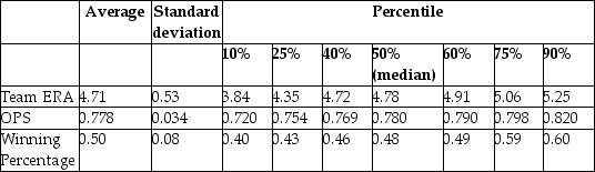
Sports economics typically looks at winning percentages of sports teams as one of various outputs,and estimates production functions by analyzing the relationship between the winning percentage and inputs.In Major League Baseball (MLB),the determinants of winning are quality pitching and batting.All 30 MLB teams for the 1999 season.Pitching quality is approximated by "Team Earned Run Average" (ERA),and hitting quality by "On Base Plus Slugging Percentage" (OPS).
Summary of the Distribution of Winning Percentage,On Base Plus Slugging Percentage,
and Team Earned Run Average for MLB in 1999
 Your regression output is:
  = -0.19 - 0.099 × teamera + 1.490 × ops,R2=0.92,SER = 0.02.
(0.08)(0.008)(0.126)
(a)Interpret the regression.Are the results statistically significant and important?
(b)There are two leagues in MLB,the American League (AL)and the National League (NL).One major difference is that the pitcher in the AL does not have to bat.Instead there is a "designated hitter" in the hitting line-up.You are concerned that,as a result,there is a different effect of pitching and hitting in the AL from the NL.To test this hypothesis,you allow the AL regression to have a different intercept and different slopes from the NL regression.You therefore create a binary variable for the American League (DAL)and estimate the following specification: = - 0.29 + 0.10 × DAL - 0.100 × teamera + 0.008 × (DAL× teamera)
(0.12)(0.24)(0.008)(0.018)
+ 1.622*ops - 0.187 *(DAL× ops),R2=0.92,SER = 0.02.
(0.163)(0.160)
What is the regression for winning percentage in the AL and NL? Next,calculate the t-statistics and say something about the statistical significance of the AL variables.Since you have allowed all slopes and the intercept to vary between the two leagues,what would the results imply if all coefficients involving DAL were statistically significant?
(c)You remember that sequentially testing the significance of slope coefficients is not the same as testing for their significance simultaneously.Hence you ask your regression package to calculate the F-statistic that all three coefficients involving the binary variable for the AL are zero.Your regression package gives a value of 0.35.Looking at the critical value from you F-table,can you reject the null hypothesis at the 1% level? Should you worry about the small sample size?
Summary of the Distribution of Winning Percentage,On Base Plus Slugging Percentage,
and Team Earned Run Average for MLB in 1999
Your regression output is: = -0.19 - 0.099 × teamera + 1.490 × ops,R2=0.92,SER = 0.02.(0.08)(0.008)(0.126)
(a)Interpret the regression.Are the results statistically significant and important?
(b)There are two leagues in MLB,the American League (AL)and the National League (NL).One major difference is that the pitcher in the AL does not have to bat.Instead there is a "designated hitter" in the hitting line-up.You are concerned that,as a result,there is a different effect of pitching and hitting in the AL from the NL.To test this hypothesis,you allow the AL regression to have a different intercept and different slopes from the NL regression.You therefore create a binary variable for the American League (DAL)and estimate the following specification:
= - 0.29 + 0.10 × DAL - 0.100 × teamera + 0.008 × (DAL× teamera)(0.12)(0.24)(0.008)(0.018)
+ 1.622*ops - 0.187 *(DAL× ops),R2=0.92,SER = 0.02.
(0.163)(0.160)
What is the regression for winning percentage in the AL and NL? Next,calculate the t-statistics and say something about the statistical significance of the AL variables.Since you have allowed all slopes and the intercept to vary between the two leagues,what would the results imply if all coefficients involving DAL were statistically significant?
(c)You remember that sequentially testing the significance of slope coefficients is not the same as testing for their significance simultaneously.Hence you ask your regression package to calculate the F-statistic that all three coefficients involving the binary variable for the AL are zero.Your regression package gives a value of 0.35.Looking at the critical value from you F-table,can you reject the null hypothesis at the 1% level? Should you worry about the small sample size?
سؤال
Females,it is said,make 70 cents to the dollar in the United States.To investigate this phenomenon,you collect data on weekly earnings from 1,744 individuals,850 females and 894 males.Next,you calculate their average weekly earnings and find that the females in your sample earned $346.98,while the males made $517.70.
(a)Calculate the female earnings in percent of the male earnings.How would you test whether or not this difference is statistically significant? Give two approaches.
(b)A peer suggests that this is consistent with the idea that there is discrimination against females in the labor market.What is your response?
(c)You recall from your textbook that additional years of experience are supposed to result in higher earnings.You reason that this is because experience is related to "on the job training." One frequently used measure for (potential)experience is "Age-Education-6." Explain the underlying rationale.Assuming,heroically,that education is constant across the 1,744 individuals,you consider regressing earnings on age and a binary variable for gender.You estimate two specifications initially: = 323.70 + 5.15 × Age - 169.78 × Female,R2=0.13,SER=274.75
(21.18)(0.55)(13.06) = 5.44 + 0.015 × Age - 0.421 × Female,R2=0.17,SER=0.75
(0.08)(0.002)(0.036)
where Earn are weekly earnings in dollars,Age is measured in years,and Female is a binary variable,which takes on the value of one if the individual is a female and is zero otherwise.Interpret each regression carefully.For a given age,how much less do females earn on average? Should you choose the second specification on grounds of the higher regression R2?
(d)Your peer points out to you that age-earning profiles typically take on an inverted U-shape.To test this idea,you add the square of age to your log-linear regression. = 3.04 + 0.147 × Age - 0.421 × Female - 0.0016 Age2,
(0.18)(0.009)(0.033)(0.0001)
R2 = 0.28,SER = 0.68
Interpret the results again.Are there strong reasons to assume that this specification is superior to the previous one? Why is the increase of the Age coefficient so large relative to its value in (c)?
(e)What other factors may play a role in earnings determination?
(a)Calculate the female earnings in percent of the male earnings.How would you test whether or not this difference is statistically significant? Give two approaches.
(b)A peer suggests that this is consistent with the idea that there is discrimination against females in the labor market.What is your response?
(c)You recall from your textbook that additional years of experience are supposed to result in higher earnings.You reason that this is because experience is related to "on the job training." One frequently used measure for (potential)experience is "Age-Education-6." Explain the underlying rationale.Assuming,heroically,that education is constant across the 1,744 individuals,you consider regressing earnings on age and a binary variable for gender.You estimate two specifications initially:
= 323.70 + 5.15 × Age - 169.78 × Female,R2=0.13,SER=274.75(21.18)(0.55)(13.06)
= 5.44 + 0.015 × Age - 0.421 × Female,R2=0.17,SER=0.75(0.08)(0.002)(0.036)
where Earn are weekly earnings in dollars,Age is measured in years,and Female is a binary variable,which takes on the value of one if the individual is a female and is zero otherwise.Interpret each regression carefully.For a given age,how much less do females earn on average? Should you choose the second specification on grounds of the higher regression R2?
(d)Your peer points out to you that age-earning profiles typically take on an inverted U-shape.To test this idea,you add the square of age to your log-linear regression.
= 3.04 + 0.147 × Age - 0.421 × Female - 0.0016 Age2,(0.18)(0.009)(0.033)(0.0001)
R2 = 0.28,SER = 0.68
Interpret the results again.Are there strong reasons to assume that this specification is superior to the previous one? Why is the increase of the Age coefficient so large relative to its value in (c)?
(e)What other factors may play a role in earnings determination?
سؤال
سؤال
There has been much debate about the impact of minimum wages on employment and unemployment.While most of the focus has been on the employment-to-population ratio of teenagers,you decide to check if aggregate state unemployment rates have been affected.Your idea is to see if state unemployment rates for the 48 contiguous U.S.states in 1985 can predict the unemployment rate for the same states in 1995,and if this prediction can be improved upon by entering a binary variable for "high impact" minimum wage states.One labor economist labeled states as high impact if a large fraction of teenagers was affected by the 1990 and 1991 federal minimum wage increases.Your first regression results in the following output:  = 3.19 + 0.27 ×
  ,R2 = 0.21,SER = 1.031
(0.56)(0.07)
(a)Sketch the regression line and add a 450 line to the graph.Interpret the regression results.What would the interpretation be if the fitted line coincided with the 450 line?
(b)Adding the binary variable DhiImpact by allowing the slope and intercept to differ,results in the following fitted line: = 4.02 + 0.16 ×
  - 3.25 × DhiImpact + 0.38 × (DhiImpact×
  ),
),
(0.66)(0.09)(0.89)(0.11)
R2 = 0.31,SER=0.987
The F-statistic for the null hypothesis that both parameters involving the high impact minimum wage variable are zero,is 42.16.Can you reject the null hypothesis that both coefficients are zero? Sketch the two regression lines together with the 450 line and interpret the results again.
(c)To check the robustness of these results,you repeat the exercise using a new binary variable for the so-called mining state (Dmining),i.e. ,the eleven states that have at least three percent of their total state earnings derived from oil,gas extraction,and coal mining,in the 1980s.This results in the following output: = 4.04 + 0.15×
  - 2.92 × Dmining + 0.37 × (Dmining ×
  ),
),
(0.65)(0.09)(0.90)(0.10)
R2 = 0.31,SER=0.997
How confident are you that the previously found effect is due to minimum wages?
= 3.19 + 0.27 × ,R2 = 0.21,SER = 1.031(0.56)(0.07)
(a)Sketch the regression line and add a 450 line to the graph.Interpret the regression results.What would the interpretation be if the fitted line coincided with the 450 line?
(b)Adding the binary variable DhiImpact by allowing the slope and intercept to differ,results in the following fitted line:
= 4.02 + 0.16 × - 3.25 × DhiImpact + 0.38 × (DhiImpact× ),(0.66)(0.09)(0.89)(0.11)
R2 = 0.31,SER=0.987
The F-statistic for the null hypothesis that both parameters involving the high impact minimum wage variable are zero,is 42.16.Can you reject the null hypothesis that both coefficients are zero? Sketch the two regression lines together with the 450 line and interpret the results again.
(c)To check the robustness of these results,you repeat the exercise using a new binary variable for the so-called mining state (Dmining),i.e. ,the eleven states that have at least three percent of their total state earnings derived from oil,gas extraction,and coal mining,in the 1980s.This results in the following output:
= 4.04 + 0.15× - 2.92 × Dmining + 0.37 × (Dmining × ),(0.65)(0.09)(0.90)(0.10)
R2 = 0.31,SER=0.997
How confident are you that the previously found effect is due to minimum wages?
سؤال
سؤال
One of the most frequently estimated equations in the macroeconomics growth literature are so-called convergence regressions.In essence the average per capita income growth rate is regressed on the beginning-of-period per capita income level to see if countries that were further behind initially,grew faster.Some macroeconomic models make this prediction,once other variables are controlled for.To investigate this matter,you collect data from 104 countries for the sample period 1960-1990 and estimate the following relationship (numbers in parentheses are for heteroskedasticity-robust standard errors):  = 0.020 - 0.360 × gpop + 0.00 4 × Educ - 0.053×RelProd60,R2=0.332,SER = 0.013
(0.009)(0.241)(0.001)(0.009)
where g6090 is the growth rate of GDP per worker for the 1960-1990 sample period,RelProd60 is the initial starting level of GDP per worker relative to the United States in 1960,gpop is the average population growth rate of the country,and Educ is educational attainment in years for 1985.
(a)What is the effect of an increase of 5 years in educational attainment? What would happen if a country could implement policies to cut population growth by one percent? Are all coefficients significant at the 5% level? If one of the coefficients is not significant,should you automatically eliminate its variable from the list of explanatory variables?
(b)The coefficient on the initial condition has to be significantly negative to suggest conditional convergence.Furthermore,the larger this coefficient,in absolute terms,the faster the convergence will take place.It has been suggested to you to interact education with the initial condition to test for additional effects of education on growth.To test for this possibility,you estimate the following regression: = 0.015 - 0.323 × gpop + 0.005 × Educ - 0.051 × RelProd60
(0.009)(0.238)(0.001)(0.013)
-0.0028 × (EducRelProd60),R2=0.346,SER = 0.013
(0.0015)
Write down the effect of an additional year of education on growth.West Germany has a value for RelProd60 of 0.57,while Brazil's value is 0.23.What is the predicted growth rate effect of adding one year of education in both countries? Does this predicted growth rate make sense?
(c)What is the implication for the speed of convergence? Is the interaction effect statistically significant?
(d)Convergence regressions are basically of the type
Δln Yt = β0 - β1 ln Y0
where △ might be the change over a longer time period,30 years,say,and the average growth rate is used on the left-hand side.You note that the equation can be rewritten as
△ln Yt = β0 - (1 - β1)ln Y0
Over a century ago,Sir Francis Galton first coined the term "regression" by analyzing the relationship between the height of children and the height of their parents.Estimating a function of the type above,he found a positive intercept and a slope between zero and one.He therefore concluded that heights would revert to the mean.Since ultimately this would imply the height of the population being the same,his result has become known as "Galton's Fallacy." Your estimate of β1 above is approximately 0.05.Do you see a parallel to Galton's Fallacy?
= 0.020 - 0.360 × gpop + 0.00 4 × Educ - 0.053×RelProd60,R2=0.332,SER = 0.013(0.009)(0.241)(0.001)(0.009)
where g6090 is the growth rate of GDP per worker for the 1960-1990 sample period,RelProd60 is the initial starting level of GDP per worker relative to the United States in 1960,gpop is the average population growth rate of the country,and Educ is educational attainment in years for 1985.
(a)What is the effect of an increase of 5 years in educational attainment? What would happen if a country could implement policies to cut population growth by one percent? Are all coefficients significant at the 5% level? If one of the coefficients is not significant,should you automatically eliminate its variable from the list of explanatory variables?
(b)The coefficient on the initial condition has to be significantly negative to suggest conditional convergence.Furthermore,the larger this coefficient,in absolute terms,the faster the convergence will take place.It has been suggested to you to interact education with the initial condition to test for additional effects of education on growth.To test for this possibility,you estimate the following regression:
= 0.015 - 0.323 × gpop + 0.005 × Educ - 0.051 × RelProd60(0.009)(0.238)(0.001)(0.013)
-0.0028 × (EducRelProd60),R2=0.346,SER = 0.013
(0.0015)
Write down the effect of an additional year of education on growth.West Germany has a value for RelProd60 of 0.57,while Brazil's value is 0.23.What is the predicted growth rate effect of adding one year of education in both countries? Does this predicted growth rate make sense?
(c)What is the implication for the speed of convergence? Is the interaction effect statistically significant?
(d)Convergence regressions are basically of the type
Δln Yt = β0 - β1 ln Y0
where △ might be the change over a longer time period,30 years,say,and the average growth rate is used on the left-hand side.You note that the equation can be rewritten as
△ln Yt = β0 - (1 - β1)ln Y0
Over a century ago,Sir Francis Galton first coined the term "regression" by analyzing the relationship between the height of children and the height of their parents.Estimating a function of the type above,he found a positive intercept and a slope between zero and one.He therefore concluded that heights would revert to the mean.Since ultimately this would imply the height of the population being the same,his result has become known as "Galton's Fallacy." Your estimate of β1 above is approximately 0.05.Do you see a parallel to Galton's Fallacy?
سؤال
In the model ln(Yi)= β0 + β1Xi + ui,the elasticity of E(Y|X)with respect to X is
A)β1X
B)β1
C)
D)Cannot be calculated because the function is non-linear
A)β1X
B)β1
C)
D)Cannot be calculated because the function is non-linear
سؤال
Earnings functions attempt to find the determinants of earnings,using both continuous and binary variables.One of the central questions analyzed in this relationship is the returns to education.
(a)Collecting data from 253 individuals,you estimate the following relationship = 0.54 + 0.083 × Educ,R2 = 0.20,SER = 0.445
(0.14)(0.011)
where Earn is average hourly earnings and Educ is years of education.
What is the effect of an additional year of schooling? If you had a strong belief that years of high school education were different from college education,how would you modify the equation? What if your theory suggested that there was a "diploma effect"?
(b)You read in the literature that there should also be returns to on-the-job training.To approximate on-the-job training,researchers often use the so called Mincer or potential experience variable,which is defined as Exper = Age - Educ - 6.Explain the reasoning behind this approximation.Is it likely to resemble years of employment for various sub-groups of the labor force?
(c)You incorporate the experience variable into your original regression = -0.01 + 0.101 × Educ + 0.033 × Exper - 0.0005 × Exper2,
(0.16)(0.012)(0.006)(0.0001)
R2 = 0.34,SER = 0.405
What is the effect of an additional year of experience for a person who is 40 years old and had 12 years of education? What about for a person who is 60 years old with the same education background?
(d)Test for the significance of each of the coefficients of the added variables.Why has the coefficient on education changed so little? Sketch the age-(log)earnings profile for workers with 8 years of education and 16 years of education.
(e)You want to find the effect of introducing two variables,gender and marital status.Accordingly you specify a binary variable that takes on the value of one for females and is zero otherwise (Female),and another binary variable that is one if the worker is married but is zero otherwise (Married).Adding these variables to the regressors results in: = 0.21 + 0.093 × Educ + 0.032 × Exper - 0.0005 × Exper2
(0.16)(0.012)(0.006)(0.0001)
- 0.289 × Female + 0.062 Married,
(0.049)(0.056)
R2 = 0.43,SER = 0.378
Are the coefficients of the two added binary variables individually statistically significant? Are they economically important? In percentage terms,how much less do females earn per hour,controlling for education and experience? How much more do married people make? What is the percentage difference in earnings between a single male and a married female? What is the marriage differential between males and females?
(f)In your final specification,you allow for the binary variables to interact.The results are as follows: = 0.14 + 0.093 × Educ + 0.032 × Exper - 0.0005 × Exper2
(0.16)(0.011)(0.006)(0.001)
- 0.158 × Female + 0.173 × Married - 0.218 × (Female × Married),
(0.075)(0.080)(0.097)
R2 = 0.44,SER = 0.375
Repeat the exercise in (e)of calculating the various percentage differences between gender and marital status.
(a)Collecting data from 253 individuals,you estimate the following relationship
= 0.54 + 0.083 × Educ,R2 = 0.20,SER = 0.445(0.14)(0.011)
where Earn is average hourly earnings and Educ is years of education.
What is the effect of an additional year of schooling? If you had a strong belief that years of high school education were different from college education,how would you modify the equation? What if your theory suggested that there was a "diploma effect"?
(b)You read in the literature that there should also be returns to on-the-job training.To approximate on-the-job training,researchers often use the so called Mincer or potential experience variable,which is defined as Exper = Age - Educ - 6.Explain the reasoning behind this approximation.Is it likely to resemble years of employment for various sub-groups of the labor force?
(c)You incorporate the experience variable into your original regression
= -0.01 + 0.101 × Educ + 0.033 × Exper - 0.0005 × Exper2,(0.16)(0.012)(0.006)(0.0001)
R2 = 0.34,SER = 0.405
What is the effect of an additional year of experience for a person who is 40 years old and had 12 years of education? What about for a person who is 60 years old with the same education background?
(d)Test for the significance of each of the coefficients of the added variables.Why has the coefficient on education changed so little? Sketch the age-(log)earnings profile for workers with 8 years of education and 16 years of education.
(e)You want to find the effect of introducing two variables,gender and marital status.Accordingly you specify a binary variable that takes on the value of one for females and is zero otherwise (Female),and another binary variable that is one if the worker is married but is zero otherwise (Married).Adding these variables to the regressors results in:
= 0.21 + 0.093 × Educ + 0.032 × Exper - 0.0005 × Exper2(0.16)(0.012)(0.006)(0.0001)
- 0.289 × Female + 0.062 Married,
(0.049)(0.056)
R2 = 0.43,SER = 0.378
Are the coefficients of the two added binary variables individually statistically significant? Are they economically important? In percentage terms,how much less do females earn per hour,controlling for education and experience? How much more do married people make? What is the percentage difference in earnings between a single male and a married female? What is the marriage differential between males and females?
(f)In your final specification,you allow for the binary variables to interact.The results are as follows:
= 0.14 + 0.093 × Educ + 0.032 × Exper - 0.0005 × Exper2(0.16)(0.011)(0.006)(0.001)
- 0.158 × Female + 0.173 × Married - 0.218 × (Female × Married),
(0.075)(0.080)(0.097)
R2 = 0.44,SER = 0.375
Repeat the exercise in (e)of calculating the various percentage differences between gender and marital status.
سؤال
Consider the following least squares specification between testscores and the student-teacher ratio:  = 557.8 + 36.42 ln (Income).According to this equation,a 1% increase income is associated with an increase in test scores of
A)0.36 points
B)36.42 points
C)557.8 points
D)cannot be determined from the information given here
= 557.8 + 36.42 ln (Income).According to this equation,a 1% increase income is associated with an increase in test scores ofA)0.36 points
B)36.42 points
C)557.8 points
D)cannot be determined from the information given here
سؤال
You have been asked by your younger sister to help her with a science fair project.During the previous years she already studied why objects float and there also was the inevitable volcano project.Having learned regression techniques recently,you suggest that she investigate the weight-height relationship of 4th to 6th graders.Her presentation topic will be to explain how people at carnivals predict weight.You collect data for roughly 100 boys and girls between the ages of nine and twelve and estimate for her the following relationship:  = 45.59 + 4.32 × Height4,R2 = 0.55,SER = 15.69
(3.81)(0.46)
where Weight is in pounds,and Height4 is inches above 4 feet.
(a)Interpret the results.
(b)You remember from the medical literature that females in the adult population are,on average,shorter than males and weigh less.You also seem to have heard that females,controlling for height,are supposed to weigh less than males.To see if this relationship holds for children,you add a binary variable (DFY)that takes on the value one for girls and is zero otherwise.You estimate the following regression function: = 36.27 + 17.33 × DFY + 5.32 × Height4 - 1.83 × (DFY × Height4),
(5.99)(7.36)(0.80)(0.90)
R2 = 0.58,SER = 15.41
Are the signs on the new coefficients as expected? Are the new coefficients individually statistically significant? Write down and sketch the regression function for boys and girls separately.
(c)The medical literature provides you with the following information for median height and weight of nine- to twelve-year-olds:
Median Height and Weight for Children,Age 9-12
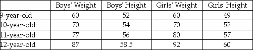 Insert two height/weight measures each for boys and girls and see how accurate your predictions are.
(d)The F-statistic for testing that the intercept and slope for boys and girls are identical is 2.92.Find the critical values at the 5% and 1% level,and make a decision.Allowing for a different intercept with an identical slope results in a t-statistic for DFY of (-0.35).Having identical intercepts but different slopes gives a t-statistic on (DFYHeight4)of (-0.35)also.Does this affect your previous conclusion?
(e)Assume that you also wanted to test if the relationship changes by age.Briefly outline how you would specify the regression including the gender binary variable and an age binary variable (Older)that takes on a value of one for eleven to twelve year olds and is zero otherwise.Indicate in a table of two rows and two columns how the estimated relationship would vary between younger girls,older girls,younger boys,and older boys.
= 45.59 + 4.32 × Height4,R2 = 0.55,SER = 15.69(3.81)(0.46)
where Weight is in pounds,and Height4 is inches above 4 feet.
(a)Interpret the results.
(b)You remember from the medical literature that females in the adult population are,on average,shorter than males and weigh less.You also seem to have heard that females,controlling for height,are supposed to weigh less than males.To see if this relationship holds for children,you add a binary variable (DFY)that takes on the value one for girls and is zero otherwise.You estimate the following regression function:
= 36.27 + 17.33 × DFY + 5.32 × Height4 - 1.83 × (DFY × Height4),(5.99)(7.36)(0.80)(0.90)
R2 = 0.58,SER = 15.41
Are the signs on the new coefficients as expected? Are the new coefficients individually statistically significant? Write down and sketch the regression function for boys and girls separately.
(c)The medical literature provides you with the following information for median height and weight of nine- to twelve-year-olds:
Median Height and Weight for Children,Age 9-12
Insert two height/weight measures each for boys and girls and see how accurate your predictions are.(d)The F-statistic for testing that the intercept and slope for boys and girls are identical is 2.92.Find the critical values at the 5% and 1% level,and make a decision.Allowing for a different intercept with an identical slope results in a t-statistic for DFY of (-0.35).Having identical intercepts but different slopes gives a t-statistic on (DFYHeight4)of (-0.35)also.Does this affect your previous conclusion?
(e)Assume that you also wanted to test if the relationship changes by age.Briefly outline how you would specify the regression including the gender binary variable and an age binary variable (Older)that takes on a value of one for eleven to twelve year olds and is zero otherwise.Indicate in a table of two rows and two columns how the estimated relationship would vary between younger girls,older girls,younger boys,and older boys.
سؤال
Pages 283-284 in your textbook contain an analysis of the "Return to Education and the Gender Gap." Column (4)in Table 8.1 displays regression results using the 2009 Current Population Survey.The equation below shows the regression result for the same specification,but using the 2005 Current Population Survey.Interpret the major results.  = 1.215 + 0.0899 × educ - 0.521 × DFemme+ 0.0180 × (DFemme×educ)
(0.018)(0.0011)(0.022)(0.0016)
+ 0.0232 × exper - 0.000368 × exper2 - 0.058 × Midwest - 0.0098 × South - 0.030 × West
(0.0008)(0.000018)(0.006)(0.0078)(0.0030)
= 1.215 + 0.0899 × educ - 0.521 × DFemme+ 0.0180 × (DFemme×educ)(0.018)(0.0011)(0.022)(0.0016)
+ 0.0232 × exper - 0.000368 × exper2 - 0.058 × Midwest - 0.0098 × South - 0.030 × West
(0.0008)(0.000018)(0.006)(0.0078)(0.0030)
سؤال
In the log-log model,the slope coefficient indicates
A)the effect that a unit change in X has on Y.
B)the elasticity of Y with respect to X.
C)ΔY / ΔX.
D) ×
×
 .
.
A)the effect that a unit change in X has on Y.
B)the elasticity of Y with respect to X.
C)ΔY / ΔX.
D)
× . سؤال
An extension of the Solow growth model that includes human capital in addition to physical capital,suggests that investment in human capital (education)will increase the wealth of a nation (per capita income).To test this hypothesis,you collect data for 104 countries and perform the following regression:  = 0.046 - 5.869 × gpop + 0.738 × SK + 0.055 × Educ,R2=0.775,SER = 0.1377
(0.079)(2.238)(0.294)(0.010)
where RelPersInc is GDP per worker relative to the United States,gpop is the average population growth rate,1980 to 1990,sK is the average investment share of GDP from 1960 to 1990,and Educ is the average educational attainment in years for 1985.Numbers in parentheses are for heteroskedasticity-robust standard errors.
(a)Interpret the results and indicate whether or not the coefficients are significantly different from zero.Do the coefficients have the expected sign?
(b)To test for equality of the coefficients between the OECD and other countries,you introduce a binary variable (DOECD),which takes on the value of one for the OECD countries and is zero otherwise.To conduct the test for equality of the coefficients,you estimate the following regression: = -0.068 - 0.063 × gpop + 0.719 × SK + 0.044 × Educ,
(0.072)(2.271)(0.365)(0.012)
0.381 × DOECD - 8.038 × (DOECD × gpop)- 0.430 × (DOECD × SK)
(0.184)(5.366) (0.768)
+0.003 × (DOECD × Educ),R2=0.845,SER = 0.116
(0.018)
Write down the two regression functions,one for the OECD countries,the other for the non-OECD countries.The F- statistic that all coefficients involving DOECD are zero,is 6.76.Find the corresponding critical value from the F table and decide whether or not the coefficients are equal across the two sets of countries.
(c)Given your answer in the previous question,you want to investigate further.You first force the same slopes across all countries,but allow the intercept to differ.That is,you reestimate the above regression but set βDOECD × gpop = βDOECD × = βDOECD × Educ = 0.The t-statistic for DOECD is 4.39.Is the coefficient,which was 0.241,statistically significant?
(d)Your final regression allows the slopes to differ in addition to the intercept.The F-statistic for βDOECD × gpop = βDOECD × = βDOECD × Educ = 0 is 1.05.What is your decision? Each one of the t-statistics is also smaller than the critical value from the standard normal table.Which test should you use?
(e)Looking at the tests in the two previous questions,what is your conclusion?
= 0.046 - 5.869 × gpop + 0.738 × SK + 0.055 × Educ,R2=0.775,SER = 0.1377(0.079)(2.238)(0.294)(0.010)
where RelPersInc is GDP per worker relative to the United States,gpop is the average population growth rate,1980 to 1990,sK is the average investment share of GDP from 1960 to 1990,and Educ is the average educational attainment in years for 1985.Numbers in parentheses are for heteroskedasticity-robust standard errors.
(a)Interpret the results and indicate whether or not the coefficients are significantly different from zero.Do the coefficients have the expected sign?
(b)To test for equality of the coefficients between the OECD and other countries,you introduce a binary variable (DOECD),which takes on the value of one for the OECD countries and is zero otherwise.To conduct the test for equality of the coefficients,you estimate the following regression:
= -0.068 - 0.063 × gpop + 0.719 × SK + 0.044 × Educ,(0.072)(2.271)(0.365)(0.012)
0.381 × DOECD - 8.038 × (DOECD × gpop)- 0.430 × (DOECD × SK)
(0.184)(5.366) (0.768)
+0.003 × (DOECD × Educ),R2=0.845,SER = 0.116
(0.018)
Write down the two regression functions,one for the OECD countries,the other for the non-OECD countries.The F- statistic that all coefficients involving DOECD are zero,is 6.76.Find the corresponding critical value from the F table and decide whether or not the coefficients are equal across the two sets of countries.
(c)Given your answer in the previous question,you want to investigate further.You first force the same slopes across all countries,but allow the intercept to differ.That is,you reestimate the above regression but set βDOECD × gpop = βDOECD ×
= βDOECD × Educ = 0.The t-statistic for DOECD is 4.39.Is the coefficient,which was 0.241,statistically significant?(d)Your final regression allows the slopes to differ in addition to the intercept.The F-statistic for βDOECD × gpop = βDOECD ×
= βDOECD × Educ = 0 is 1.05.What is your decision? Each one of the t-statistics is also smaller than the critical value from the standard normal table.Which test should you use?(e)Looking at the tests in the two previous questions,what is your conclusion?
سؤال
سؤال
Labor economists have extensively researched the determinants of earnings.Investment in human capital,measured in years of education,and on the job training are some of the most important explanatory variables in this research.You decide to apply earnings functions to the field of sports economics by finding the determinants for baseball pitcher salaries.You collect data on 455 pitchers for the 1998 baseball season and estimate the following equation using OLS and heteroskedasticity-robust standard errors:  = 12.45 + 0.052 × Years + 0.00089 × Innings + 0.0032 × Saves
(0.08)(0.026)(0.00020)(0.0018)
- 0.0085 × ERA,R2 = 0.45,SER = 0.874
(0.0168)
where Earn is annual salary in dollars,Years is number of years in the major leagues,Innings is number of innings pitched during the career before the 1998 season,Saves is number of saves during the career before the 1998 season,and ERA is the earned run average before the 1998 season.
(a)What happens to earnings when the pitcher stays in the league for one additional year? Compare the salaries of two relievers,one with 10 more saves than the other.What effect does pitching 100 more innings have on the salary of the pitcher? What effect does reducing his ERA by 1.5? Do the signs correspond to your expectations? Explain.
(b)Are the individual coefficients statistically significant? Indicate the level of significance you used and the type of alternative hypothesis you considered.
(c)Although you are quite impressed with the fit of the regression,someone suggests that you should include the square of years and innings as additional explanatory variables.Your results change as follows: = 12.15 + 0.160 × Years + 0.00268 × Innings + 0.0063 × Saves
(0.05)(0.039)(0.00030)(0.0010)
- 0.0584 × ERA - 0.0165 × Years2 - 0.00000045 × Innings2
(0.0165)(0.0026)(0.00000012)
R2 = 0.69,SER = 0.666
What is her reasoning? Are the coefficients of the quadratic terms statistically significant? Are they meaningful?
(d)Calculate the effect of moving from two to three years,as opposed to from 12 to 13 years.
(e)You also decide to test the specification for stability across leagues (National League and American League)by including a dummy variable for the National League and allowing the intercept and all slopes to differ.The resulting F-statistic for restricting all coefficients that involve the National League dummy variable to zero,is 0.40.Compare this to the relevant critical value from the table and decide whether or not these additional variables should be included.
= 12.45 + 0.052 × Years + 0.00089 × Innings + 0.0032 × Saves(0.08)(0.026)(0.00020)(0.0018)
- 0.0085 × ERA,R2 = 0.45,SER = 0.874
(0.0168)
where Earn is annual salary in dollars,Years is number of years in the major leagues,Innings is number of innings pitched during the career before the 1998 season,Saves is number of saves during the career before the 1998 season,and ERA is the earned run average before the 1998 season.
(a)What happens to earnings when the pitcher stays in the league for one additional year? Compare the salaries of two relievers,one with 10 more saves than the other.What effect does pitching 100 more innings have on the salary of the pitcher? What effect does reducing his ERA by 1.5? Do the signs correspond to your expectations? Explain.
(b)Are the individual coefficients statistically significant? Indicate the level of significance you used and the type of alternative hypothesis you considered.
(c)Although you are quite impressed with the fit of the regression,someone suggests that you should include the square of years and innings as additional explanatory variables.Your results change as follows:
= 12.15 + 0.160 × Years + 0.00268 × Innings + 0.0063 × Saves(0.05)(0.039)(0.00030)(0.0010)
- 0.0584 × ERA - 0.0165 × Years2 - 0.00000045 × Innings2
(0.0165)(0.0026)(0.00000012)
R2 = 0.69,SER = 0.666
What is her reasoning? Are the coefficients of the quadratic terms statistically significant? Are they meaningful?
(d)Calculate the effect of moving from two to three years,as opposed to from 12 to 13 years.
(e)You also decide to test the specification for stability across leagues (National League and American League)by including a dummy variable for the National League and allowing the intercept and all slopes to differ.The resulting F-statistic for restricting all coefficients that involve the National League dummy variable to zero,is 0.40.Compare this to the relevant critical value from the table and decide whether or not these additional variables should be included.
سؤال
Assume that you had estimated the following quadratic regression model  = 607.3 + 3.85 Income - 0.0423 Income2.If income increased from 10 to 11 ($10,000 to $11,000),then the predicted effect on testscores would be
A)3.85
B)3.85-0.0423
C)Cannot be calculated because the function is non-linear
D)2.96
= 607.3 + 3.85 Income - 0.0423 Income2.If income increased from 10 to 11 ($10,000 to $11,000),then the predicted effect on testscores would beA)3.85
B)3.85-0.0423
C)Cannot be calculated because the function is non-linear
D)2.96
سؤال
Consider the polynomial regression model of degree Yi = β0 + β1Xi + β2  + ...+ βr
  + ui.According to the null hypothesis that the regression is linear and the alternative that is a polynomial of degree r corresponds to
A)H0: βr = 0 vs.βr ≠ 0
B)H0: βr = 0 vs.β1 ≠ 0
C)H0: β3 = 0,... ,βr = 0,vs.H1: all βj ≠ 0,j = 3,... ,r
D)H0: β2 = 0,β3 = 0 ... ,βr = 0,vs.H1: at least one βj ≠ 0,j = 2,... ,r
+ ...+ βr + ui.According to the null hypothesis that the regression is linear and the alternative that is a polynomial of degree r corresponds toA)H0: βr = 0 vs.βr ≠ 0
B)H0: βr = 0 vs.β1 ≠ 0
C)H0: β3 = 0,... ,βr = 0,vs.H1: all βj ≠ 0,j = 3,... ,r
D)H0: β2 = 0,β3 = 0 ... ,βr = 0,vs.H1: at least one βj ≠ 0,j = 2,... ,r
سؤال
سؤال
You have learned that earnings functions are one of the most investigated relationships in economics.These typically relate the logarithm of earnings to a series of explanatory variables such as education,work experience,gender,race,etc.
(a)Why do you think that researchers have preferred a log-linear specification over a linear specification? In addition to the interpretation of the slope coefficients,also think about the distribution of the error term.
(b)To establish age-earnings profiles,you regress ln(Earn)on Age,where Earn is weekly earnings in dollars,and Age is in years.Plotting the residuals of the regression against age for 1,744 individuals looks as shown in the figure: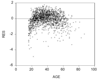 Do you sense a problem?
(c)You decide,given your knowledge of age-earning profiles,to allow the regression line to differ for the below and above 40 years age category.Accordingly you create a binary variable,Dage,that takes the value one for age 39 and below,and is zero otherwise.Estimating the earnings equation results in the following output (using heteroskedasticity-robust standard errors): = 6.92 - 3.13 × Dage - 0.019 × Age + 0.085 × (Dage × Age),R2=0.20,SER =0.721.
(38.33)(0.22)(0.004)(0.005)
Sketch both regression lines: one for the age category 39 years and under,and one for 40 and above.Does it make sense to have a negative sign on the Age coefficient? Predict the ln(earnings)for a 30 year old and a 50 year old.What is the percentage difference between these two?
(d)The F-statistic for the hypothesis that both slopes and intercepts are the same is 124.43.Can you reject the null hypothesis?
(e)What other functional forms should you consider?
(a)Why do you think that researchers have preferred a log-linear specification over a linear specification? In addition to the interpretation of the slope coefficients,also think about the distribution of the error term.
(b)To establish age-earnings profiles,you regress ln(Earn)on Age,where Earn is weekly earnings in dollars,and Age is in years.Plotting the residuals of the regression against age for 1,744 individuals looks as shown in the figure:
Do you sense a problem?(c)You decide,given your knowledge of age-earning profiles,to allow the regression line to differ for the below and above 40 years age category.Accordingly you create a binary variable,Dage,that takes the value one for age 39 and below,and is zero otherwise.Estimating the earnings equation results in the following output (using heteroskedasticity-robust standard errors):
= 6.92 - 3.13 × Dage - 0.019 × Age + 0.085 × (Dage × Age),R2=0.20,SER =0.721.(38.33)(0.22)(0.004)(0.005)
Sketch both regression lines: one for the age category 39 years and under,and one for 40 and above.Does it make sense to have a negative sign on the Age coefficient? Predict the ln(earnings)for a 30 year old and a 50 year old.What is the percentage difference between these two?
(d)The F-statistic for the hypothesis that both slopes and intercepts are the same is 124.43.Can you reject the null hypothesis?
(e)What other functional forms should you consider?
سؤال
In the model Yi = β0 + β1X1 + β2X2 + β3(X1 × X2)+ ui,the expected effect  is
is
A)β1 + β3X2.
B)β1.
C)β1 + β3.
D)β1 + β3X1.
isA)β1 + β3X2.
B)β1.
C)β1 + β3.
D)β1 + β3X1.
سؤال
Using a spreadsheet program such as Excel,plot the following logistic regression function with a single X,  i =
i =  ,where
  0 = - 4.13 and
  1 = 5.37.Enter values of X in the first column starting from 0 and then incrementing these by 0.1 until you reach 2.0.Then enter the logistic function formula in the next column.Finally produce a scatter plot,connecting the predicted values with a line.
i = ,where 0 = - 4.13 and 1 = 5.37.Enter values of X in the first column starting from 0 and then incrementing these by 0.1 until you reach 2.0.Then enter the logistic function formula in the next column.Finally produce a scatter plot,connecting the predicted values with a line. سؤال
In the case of perfect multicollinearity,OLS is unable to estimate the slope coefficients of the variables involved.Assume that you have included both X1 and X2 as explanatory variables,and that X2 = X  ,so that there is an exact relationship between two explanatory variables.Does this pose a problem for estimation?
,so that there is an exact relationship between two explanatory variables.Does this pose a problem for estimation? سؤال
In estimating the original relationship between money wage growth and the unemployment rate,Phillips used United Kingdom data from 1861 to 1913 to fit a curve of the following functional form
( + β0)= β1 ×
  × eu,
× eu,
where is the percentage change in money wages and ur is the unemployment rate.Sketch the function.What role does β0 play? Can you find a linear transformation that allows you to estimate the above function using OLS? If,after taking logarithms on both sides of the equation,you tried to estimate β1 and β2 using OLS by choosing different values for β0 by "trial and error procedure" (Phillips's words),what sort of problem might you run into with the left-hand side variable for some of the observations?
(
+ β0)= β1 × × eu,where
is the percentage change in money wages and ur is the unemployment rate.Sketch the function.What role does β0 play? Can you find a linear transformation that allows you to estimate the above function using OLS? If,after taking logarithms on both sides of the equation,you tried to estimate β1 and β2 using OLS by choosing different values for β0 by "trial and error procedure" (Phillips's words),what sort of problem might you run into with the left-hand side variable for some of the observations? سؤال
سؤال
سؤال
سؤال
Many countries that experience hyperinflation do not have market-determined interest rates.As a result,some authors have substituted future inflation rates into money demand equations of the following type as a proxy: 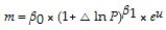 (m is real money,and P is the consumer price index).
Income is typically omitted since movements in it are dwarfed by money growth and the inflation rate.Authors have then interpreted β1 as the "semi-elasticity" of the inflation rate.Do you see any problems with this interpretation?
(m is real money,and P is the consumer price index).Income is typically omitted since movements in it are dwarfed by money growth and the inflation rate.Authors have then interpreted β1 as the "semi-elasticity" of the inflation rate.Do you see any problems with this interpretation?
سؤال
Suggest a transformation in the variables that will linearize the deterministic part of the population regression functions below.Write the resulting regression function in a form that can be estimated by using OLS.
(a)Yi = β0
 (b)Yi =
  (c)Yi =
  (d)Yi = β0

(a)Yi = β0
(b)Yi = (c)Yi = (d)Yi = β0 سؤال
سؤال
Show that for the following regression model
Yt = where t is a time trend,which takes on the values 1,2,…,T,β1 represents the instantaneous ("continuous compounding")growth rate.Show how this rate is related to the proportionate rate of growth,which is calculated from the relationship
Yt = Y0 × (1 + g)t
when time is measured in discrete intervals.
Yt =
where t is a time trend,which takes on the values 1,2,…,T,β1 represents the instantaneous ("continuous compounding")growth rate.Show how this rate is related to the proportionate rate of growth,which is calculated from the relationshipYt = Y0 × (1 + g)t
when time is measured in discrete intervals.
سؤال
The figure shows is a plot and a fitted linear regression line of the age-earnings profile of 1,744 individuals,taken from the Current Population Survey. 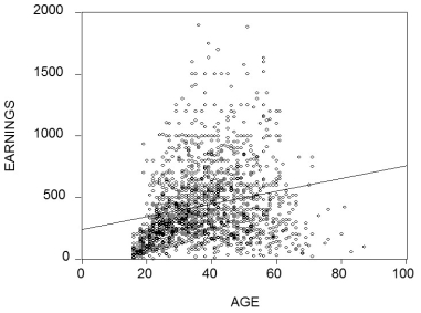 (a)Describe the problems in predicting earnings using the fitted line.What would the pattern of the residuals look like for the age category under 40?
(b)What alternative functional form might fit the data better?
(c)What other variables might you want to consider in specifying the determinants of earnings?
(a)Describe the problems in predicting earnings using the fitted line.What would the pattern of the residuals look like for the age category under 40?(b)What alternative functional form might fit the data better?
(c)What other variables might you want to consider in specifying the determinants of earnings?
سؤال
Being a competitive female swimmer,you wonder if women will ever be able to beat the time of the male gold medal winner.To investigate this question,you collect data for the Olympic Games since 1910.At first you consider including various distances,a binary variable for Mark Spitz,and another binary variable for the arrival and presence of East German female swimmers,but in the end decide on a simple linear regression.Your dependent variable is the ratio of the fastest women's time to the fastest men's time in the 100 m backstroke,and the explanatory variable is the year of the Olympics.The regression result is as follows,  = 4.42 - 0.0017 × Olympics,
where TFoverM is the relative time of the gold medal winner,and Olympics is the year of the Olympic Games.What is your prediction when females will catch up to men in this discipline? Does this sound plausible? What other functional form might you want to consider?
= 4.42 - 0.0017 × Olympics,where TFoverM is the relative time of the gold medal winner,and Olympics is the year of the Olympic Games.What is your prediction when females will catch up to men in this discipline? Does this sound plausible? What other functional form might you want to consider?
سؤال
سؤال
Indicate whether or not you can linearize the regression functions below so that OLS estimation methods can be applied:
(a)Yi = (b)Yi =

 + ui
+ ui
(a)Yi =
(b)Yi = + ui سؤال
سؤال
سؤال
Earnings functions attempt to predict the log of earnings from a set of explanatory variables,both binary and continuous.You have allowed for an interaction between two continuous variables: education and tenure with the current employer.Your estimated equation is of the following type:  =
=  0 +
0 +  1 × Femme +
  2 × Educ +
  3 × Tenure +
  4 x (Educ × Tenure)+ ∙∙∙
where Femme is a binary variable taking on the value of one for females and is zero otherwise,Educ is the number of years of education,and tenure is continuous years of work with the current employer.What is the effect of an additional year of education on earnings ("returns to education")for men? For women? If you allowed for the returns to education to differ for males and females,how would you respecify the above equation? What is the effect of an additional year of tenure with a current employer on earnings?
= 0 + 1 × Femme + 2 × Educ + 3 × Tenure + 4 x (Educ × Tenure)+ ∙∙∙where Femme is a binary variable taking on the value of one for females and is zero otherwise,Educ is the number of years of education,and tenure is continuous years of work with the current employer.What is the effect of an additional year of education on earnings ("returns to education")for men? For women? If you allowed for the returns to education to differ for males and females,how would you respecify the above equation? What is the effect of an additional year of tenure with a current employer on earnings?
سؤال
سؤال
The textbook shows that ln(x + Δx)- ln(x)≅  .Show that this is equivalent to the following approximation ln(1 + y)≅ y if y is small.You use this idea to estimate a demand for money function,which is of the form m = β0 ×
  ×,
×,  × eu where m is the quantity of (real)money,GDP is the value of (real)Gross Domestic Product,and R is the nominal interest rate.You collect the quarterly data from the Federal Reserve Bank of St.Louis data bank ("FRED"),which lists the money supply and GDP in billions of dollars,prices as an index,and nominal interest rates in percentage points per year
You generate the variables in your regression program as follows: m = (money supply)/price index;GDP = (Gross Domestic Product/Price Index),and R = nominal interest rate in percentage points per annum.Next you perform the log-transformations on the real money supply,real GDP,and on (1+R).Can you for see a problem in using this transformation?
.Show that this is equivalent to the following approximation ln(1 + y)≅ y if y is small.You use this idea to estimate a demand for money function,which is of the form m = β0 × ×, × eu where m is the quantity of (real)money,GDP is the value of (real)Gross Domestic Product,and R is the nominal interest rate.You collect the quarterly data from the Federal Reserve Bank of St.Louis data bank ("FRED"),which lists the money supply and GDP in billions of dollars,prices as an index,and nominal interest rates in percentage points per yearYou generate the variables in your regression program as follows: m = (money supply)/price index;GDP = (Gross Domestic Product/Price Index),and R = nominal interest rate in percentage points per annum.Next you perform the log-transformations on the real money supply,real GDP,and on (1+R).Can you for see a problem in using this transformation?
سؤال
سؤال
سؤال
Table 8.1 on page 284 of your textbook displays the following estimated earnings function in column (4):  = 1.503 + 0.1032 × educ - 0.451 × DFemme + 0.0143 × (DFemme×educ)
(0.023)(0.0012)(0.024)(0.0017)
+ 0.0232 × exper - 0.000368 × exper2 - 0.058 × Midwest - 0.0098 × South - 0.030 × West
(0.0012)(0.000023)(0.006)(0.006)(0.007)
n = 52.790, 2 = 0.267
Given that the potential experience variable (exper)is defined as (Age-Education-6)find the age at which individuals with a high school degree (12 years of education)and with a college degree (16 years of education)have maximum earnings,holding all other factors constant.
= 1.503 + 0.1032 × educ - 0.451 × DFemme + 0.0143 × (DFemme×educ)(0.023)(0.0012)(0.024)(0.0017)
+ 0.0232 × exper - 0.000368 × exper2 - 0.058 × Midwest - 0.0098 × South - 0.030 × West
(0.0012)(0.000023)(0.006)(0.006)(0.007)
n = 52.790,
2 = 0.267Given that the potential experience variable (exper)is defined as (Age-Education-6)find the age at which individuals with a high school degree (12 years of education)and with a college degree (16 years of education)have maximum earnings,holding all other factors constant.

فتح الحزمة
قم بالتسجيل لفتح البطاقات في هذه المجموعة!
Unlock Deck
Unlock Deck
1/62
العب
ملء الشاشة (f)
Deck 8: Nonlinear Regression Functions
1
A polynomial regression model is specified as:
A)Yi = β0 + β1Xi + β2X + ∙∙∙ + βrX
+ ui.
B)Yi = β0 + β1Xi + β Xi + ∙∙∙ + β
Xi + ui.
C)Yi = β0 + β1Xi + β2Y + ∙∙∙ + βrY
+ ui.
D)Yi = β0 + β1X1i + β2X2 + β3 (X1i × X2i)+ ui.
A)Yi = β0 + β1Xi + β2X
+ ∙∙∙ + βrX + ui.B)Yi = β0 + β1Xi + β
Xi + ∙∙∙ + β Xi + ui.C)Yi = β0 + β1Xi + β2Y
+ ∙∙∙ + βrY + ui.D)Yi = β0 + β1X1i + β2X2 + β3 (X1i × X2i)+ ui.
A
2
The exponential function
A)is the inverse of the natural logarithm function.
B)does not play an important role in modeling nonlinear regression functions in econometrics.
C)can be written as exp(ex).
D)is ex,where e is 3.1415….
A)is the inverse of the natural logarithm function.
B)does not play an important role in modeling nonlinear regression functions in econometrics.
C)can be written as exp(ex).
D)is ex,where e is 3.1415….
A
3
(Requires Calculus)In the equation = 607.3 + 3.85 Income - 0.0423Income2,the following income level results in the maximum test score
A)607.3.
B)91.02.
C)45.50.
D)cannot be determined without a plot of the data.
= 607.3 + 3.85 Income - 0.0423Income2,the following income level results in the maximum test scoreA)607.3.
B)91.02.
C)45.50.
D)cannot be determined without a plot of the data.
C
4
The interpretation of the slope coefficient in the model Yi = β0 + β1 ln(Xi)+ ui is as follows:
A)a 1% change in X is associated with a β1 % change in Y.
B)a 1% change in X is associated with a change in Y of 0.01 β1.
C)a change in X by one unit is associated with a β1 100% change in Y.
D)a change in X by one unit is associated with a β1 change in Y.
A)a 1% change in X is associated with a β1 % change in Y.
B)a 1% change in X is associated with a change in Y of 0.01 β1.
C)a change in X by one unit is associated with a β1 100% change in Y.
D)a change in X by one unit is associated with a β1 change in Y.
فتح الحزمة
افتح القفل للوصول البطاقات البالغ عددها 62 في هذه المجموعة.
فتح الحزمة
k this deck
5
The interpretation of the slope coefficient in the model ln(Yi)= β0 + β1Xi + ui is as follows:
A)a 1% change in X is associated with a β1 % change in Y.
B)a change in X by one unit is associated with a 100 β1 % change in Y.
C)a 1% change in X is associated with a change in Y of 0.01 β1.
D)a change in X by one unit is associated with a β1 change in Y.
A)a 1% change in X is associated with a β1 % change in Y.
B)a change in X by one unit is associated with a 100 β1 % change in Y.
C)a 1% change in X is associated with a change in Y of 0.01 β1.
D)a change in X by one unit is associated with a β1 change in Y.
فتح الحزمة
افتح القفل للوصول البطاقات البالغ عددها 62 في هذه المجموعة.
فتح الحزمة
k this deck
6
Including an interaction term between two independent variables,X1 and X2,allows for the following except:
A)the interaction term lets the effect on Y of a change in X1 depend on the value of X2.
B)the interaction term coefficient is the effect of a unit increase in X1 and X2 above and beyond the sum of the individual effects of a unit increase in the two variables alone.
C)the interaction term coefficient is the effect of a unit increase in .
D)the interaction term lets the effect on Y of a change in X2 depend on the value of X1.
A)the interaction term lets the effect on Y of a change in X1 depend on the value of X2.
B)the interaction term coefficient is the effect of a unit increase in X1 and X2 above and beyond the sum of the individual effects of a unit increase in the two variables alone.
C)the interaction term coefficient is the effect of a unit increase in
.D)the interaction term lets the effect on Y of a change in X2 depend on the value of X1.
فتح الحزمة
افتح القفل للوصول البطاقات البالغ عددها 62 في هذه المجموعة.
فتح الحزمة
k this deck
7
An example of a quadratic regression model is
A)Yi = β0 + β1X + β2Y2 + ui.
B)Yi = β0 + β1ln(X)+ ui.
C)Yi = β0 + β1X + β2X2 + ui.
D) = β0 + β1X + ui.
A)Yi = β0 + β1X + β2Y2 + ui.
B)Yi = β0 + β1ln(X)+ ui.
C)Yi = β0 + β1X + β2X2 + ui.
D)
= β0 + β1X + ui. فتح الحزمة
افتح القفل للوصول البطاقات البالغ عددها 62 في هذه المجموعة.
فتح الحزمة
k this deck
8
The best way to interpret polynomial regressions is to
A)take a derivative of Y with respect to the relevant X.
B)plot the estimated regression function and to calculate the estimated effect on Y associated with a change in X for one or more values of X.
C)look at the t-statistics for the relevant coefficients.
D)analyze the standard error of estimated effect.
فتح الحزمة
افتح القفل للوصول البطاقات البالغ عددها 62 في هذه المجموعة.
فتح الحزمة
k this deck
9
The following interactions between binary and continuous variables are possible,with the exception of
A)Yi = β0 + β1Xi + β2Di + β3(Xi × Di)+ ui.
B)Yi = β0 + β1Xi + β2(Xi × Di)+ ui.
C)Yi = (β0 + Di)+ β1Xi + ui.
D)Yi = β0 + β1Xi + β2Di + ui.
A)Yi = β0 + β1Xi + β2Di + β3(Xi × Di)+ ui.
B)Yi = β0 + β1Xi + β2(Xi × Di)+ ui.
C)Yi = (β0 + Di)+ β1Xi + ui.
D)Yi = β0 + β1Xi + β2Di + ui.
فتح الحزمة
افتح القفل للوصول البطاقات البالغ عددها 62 في هذه المجموعة.
فتح الحزمة
k this deck
10
To decide whether Yi = β0 + β1X + ui or ln(Yi)= β0 + β1X + ui fits the data better,you cannot consult the regression R2 because
A)ln(Y)may be negative for 0B)the TSS are not measured in the same units between the two models.
C)the slope no longer indicates the effect of a unit change of X on Y in the log-linear model.
D)the regression R2 can be greater than one in the second model.
A)ln(Y)may be negative for 0
C)the slope no longer indicates the effect of a unit change of X on Y in the log-linear model.
D)the regression R2 can be greater than one in the second model.
فتح الحزمة
افتح القفل للوصول البطاقات البالغ عددها 62 في هذه المجموعة.
فتح الحزمة
k this deck
11
An example of the interaction term between two independent,continuous variables is
A)Yi = β0 + β1Xi + β2Di + β3(Xi × Di)+ ui.
B)Yi = β0 + β1X1i + β2X2i + ui.
C)Yi = β0 + β1D1i + β2D2i + β3 (D1i × D2i)+ ui.
D)Yi = β0 + β1X1i + β2X2i + β3(X1i × X2i)+ ui.
A)Yi = β0 + β1Xi + β2Di + β3(Xi × Di)+ ui.
B)Yi = β0 + β1X1i + β2X2i + ui.
C)Yi = β0 + β1D1i + β2D2i + β3 (D1i × D2i)+ ui.
D)Yi = β0 + β1X1i + β2X2i + β3(X1i × X2i)+ ui.
فتح الحزمة
افتح القفل للوصول البطاقات البالغ عددها 62 في هذه المجموعة.
فتح الحزمة
k this deck
12
A nonlinear function
A)makes little sense,because variables in the real world are related linearly.
B)can be adequately described by a straight line between the dependent variable and one of the explanatory variables.
C)is a concept that only applies to the case of a single or two explanatory variables since you cannot draw a line in four dimensions.
D)is a function with a slope that is not constant.
فتح الحزمة
افتح القفل للوصول البطاقات البالغ عددها 62 في هذه المجموعة.
فتح الحزمة
k this deck
13
To test whether or not the population regression function is linear rather than a polynomial of order r,
A)check whether the regression R2 for the polynomial regression is higher than that of the linear regression.
B)compare the TSS from both regressions.
C)look at the pattern of the coefficients: if they change from positive to negative to positive,etc. ,then the polynomial regression should be used.
D)use the test of (r-1)restrictions using the F-statistic.
فتح الحزمة
افتح القفل للوصول البطاقات البالغ عددها 62 في هذه المجموعة.
فتح الحزمة
k this deck
14
In the case of regression with interactions,the coefficient of a binary variable should be interpreted as follows:
A)there are really problems in interpreting these,since the ln(0)is not defined.
B)for the case of interacted regressors,the binary variable coefficient represents the various intercepts for the case when the binary variable equals one.
C)first set all explanatory variables to one,with the exception of the binary variables.Then allow for each of the binary variables to take on the value of one sequentially.The resulting predicted value indicates the effect of the binary variable.
D)first compute the expected values of Y for each possible case described by the set of binary variables.Next compare these expected values.Each coefficient can then be expressed either as an expected value or as the difference between two or more expected values.
فتح الحزمة
افتح القفل للوصول البطاقات البالغ عددها 62 في هذه المجموعة.
فتح الحزمة
k this deck
15
You have estimated the following equation: = 607.3 + 3.85 Income - 0.0423 Income2, where TestScore is the average of the reading and math scores on the Stanford 9 standardized test administered to 5th grade students in 420 California school districts in 1998 and 1999.Income is the average annual per capita income in the school district,measured in thousands of 1998 dollars.The equation
A)suggests a positive relationship between test scores and income for most of the sample.
B)is positive until a value of Income of 610.81.
C)does not make much sense since the square of income is entered.
D)suggests a positive relationship between test scores and income for all of the sample.
= 607.3 + 3.85 Income - 0.0423 Income2, where TestScore is the average of the reading and math scores on the Stanford 9 standardized test administered to 5th grade students in 420 California school districts in 1998 and 1999.Income is the average annual per capita income in the school district,measured in thousands of 1998 dollars.The equationA)suggests a positive relationship between test scores and income for most of the sample.
B)is positive until a value of Income of 610.81.
C)does not make much sense since the square of income is entered.
D)suggests a positive relationship between test scores and income for all of the sample.
فتح الحزمة
افتح القفل للوصول البطاقات البالغ عددها 62 في هذه المجموعة.
فتح الحزمة
k this deck
16
The binary variable interaction regression
A)can only be applied when there are two binary variables,but not three or more.
B)is the same as testing for differences in means.
C)cannot be used with logarithmic regression functions because ln(0)is not defined.
D)allows the effect of changing one of the binary independent variables to depend on the value of the other binary variable.
فتح الحزمة
افتح القفل للوصول البطاقات البالغ عددها 62 في هذه المجموعة.
فتح الحزمة
k this deck
17
The interpretation of the slope coefficient in the model ln(Yi)= β0 + β1 ln(Xi)+ ui is as follows:
A)a 1% change in X is associated with a β1 % change in Y.
B)a change in X by one unit is associated with a β1 change in Y.
C)a change in X by one unit is associated with a 100 β1 % change in Y.
D)a 1% change in X is associated with a change in Y of 0.01 β1.
A)a 1% change in X is associated with a β1 % change in Y.
B)a change in X by one unit is associated with a β1 change in Y.
C)a change in X by one unit is associated with a 100 β1 % change in Y.
D)a 1% change in X is associated with a change in Y of 0.01 β1.
فتح الحزمة
افتح القفل للوصول البطاقات البالغ عددها 62 في هذه المجموعة.
فتح الحزمة
k this deck
18
For the polynomial regression model,
A)you need new estimation techniques since the OLS assumptions do not apply any longer.
B)the techniques for estimation and inference developed for multiple regression can be applied.
C)you can still use OLS estimation techniques,but the t-statistics do not have an asymptotic normal distribution.
D)the critical values from the normal distribution have to be changed to 1.962,1.963,etc.
فتح الحزمة
افتح القفل للوصول البطاقات البالغ عددها 62 في هذه المجموعة.
فتح الحزمة
k this deck
19
In nonlinear models,the expected change in the dependent variable for a change in one of the explanatory variables is given by
A)△Y = f(X1 + X1,X2,...Xk).
B)△Y = f(X1 + △X1,X2 + △X2,... ,Xk+ △Xk)- f(X1,X2,...Xk).
C)△Y = f(X1 + △X1,X2,... ,Xk)- f(X1,X2,...Xk).
D)△Y = f(X1 + X1,X2,... ,Xk)- f(X1,X2,...Xk).
A)△Y = f(X1 + X1,X2,...Xk).
B)△Y = f(X1 + △X1,X2 + △X2,... ,Xk+ △Xk)- f(X1,X2,...Xk).
C)△Y = f(X1 + △X1,X2,... ,Xk)- f(X1,X2,...Xk).
D)△Y = f(X1 + X1,X2,... ,Xk)- f(X1,X2,...Xk).
فتح الحزمة
افتح القفل للوصول البطاقات البالغ عددها 62 في هذه المجموعة.
فتح الحزمة
k this deck
20
The following are properties of the logarithm function with the exception of
A)ln(1/ x)= -ln(x).
B)ln(a + x)= ln(a)+ ln(x).
C)ln(ax)= ln(a)+ ln(x).
D)ln(xa)a ln(x).
A)ln(1/ x)= -ln(x).
B)ln(a + x)= ln(a)+ ln(x).
C)ln(ax)= ln(a)+ ln(x).
D)ln(xa)a ln(x).
فتح الحزمة
افتح القفل للوصول البطاقات البالغ عددها 62 في هذه المجموعة.
فتح الحزمة
k this deck
21
Sports economics typically looks at winning percentages of sports teams as one of various outputs,and estimates production functions by analyzing the relationship between the winning percentage and inputs.In Major League Baseball (MLB),the determinants of winning are quality pitching and batting.All 30 MLB teams for the 1999 season.Pitching quality is approximated by "Team Earned Run Average" (ERA),and hitting quality by "On Base Plus Slugging Percentage" (OPS).
Summary of the Distribution of Winning Percentage,On Base Plus Slugging Percentage,
and Team Earned Run Average for MLB in 1999
Your regression output is: = -0.19 - 0.099 × teamera + 1.490 × ops,R2=0.92,SER = 0.02.
(0.08)(0.008)(0.126)
(a)Interpret the regression.Are the results statistically significant and important?
(b)There are two leagues in MLB,the American League (AL)and the National League (NL).One major difference is that the pitcher in the AL does not have to bat.Instead there is a "designated hitter" in the hitting line-up.You are concerned that,as a result,there is a different effect of pitching and hitting in the AL from the NL.To test this hypothesis,you allow the AL regression to have a different intercept and different slopes from the NL regression.You therefore create a binary variable for the American League (DAL)and estimate the following specification: = - 0.29 + 0.10 × DAL - 0.100 × teamera + 0.008 × (DAL× teamera)
(0.12)(0.24)(0.008)(0.018)
+ 1.622*ops - 0.187 *(DAL× ops),R2=0.92,SER = 0.02.
(0.163)(0.160)
What is the regression for winning percentage in the AL and NL? Next,calculate the t-statistics and say something about the statistical significance of the AL variables.Since you have allowed all slopes and the intercept to vary between the two leagues,what would the results imply if all coefficients involving DAL were statistically significant?
(c)You remember that sequentially testing the significance of slope coefficients is not the same as testing for their significance simultaneously.Hence you ask your regression package to calculate the F-statistic that all three coefficients involving the binary variable for the AL are zero.Your regression package gives a value of 0.35.Looking at the critical value from you F-table,can you reject the null hypothesis at the 1% level? Should you worry about the small sample size?
Summary of the Distribution of Winning Percentage,On Base Plus Slugging Percentage,
and Team Earned Run Average for MLB in 1999
Your regression output is: = -0.19 - 0.099 × teamera + 1.490 × ops,R2=0.92,SER = 0.02.(0.08)(0.008)(0.126)
(a)Interpret the regression.Are the results statistically significant and important?
(b)There are two leagues in MLB,the American League (AL)and the National League (NL).One major difference is that the pitcher in the AL does not have to bat.Instead there is a "designated hitter" in the hitting line-up.You are concerned that,as a result,there is a different effect of pitching and hitting in the AL from the NL.To test this hypothesis,you allow the AL regression to have a different intercept and different slopes from the NL regression.You therefore create a binary variable for the American League (DAL)and estimate the following specification:
= - 0.29 + 0.10 × DAL - 0.100 × teamera + 0.008 × (DAL× teamera)(0.12)(0.24)(0.008)(0.018)
+ 1.622*ops - 0.187 *(DAL× ops),R2=0.92,SER = 0.02.
(0.163)(0.160)
What is the regression for winning percentage in the AL and NL? Next,calculate the t-statistics and say something about the statistical significance of the AL variables.Since you have allowed all slopes and the intercept to vary between the two leagues,what would the results imply if all coefficients involving DAL were statistically significant?
(c)You remember that sequentially testing the significance of slope coefficients is not the same as testing for their significance simultaneously.Hence you ask your regression package to calculate the F-statistic that all three coefficients involving the binary variable for the AL are zero.Your regression package gives a value of 0.35.Looking at the critical value from you F-table,can you reject the null hypothesis at the 1% level? Should you worry about the small sample size?
فتح الحزمة
افتح القفل للوصول البطاقات البالغ عددها 62 في هذه المجموعة.
فتح الحزمة
k this deck
22
Females,it is said,make 70 cents to the dollar in the United States.To investigate this phenomenon,you collect data on weekly earnings from 1,744 individuals,850 females and 894 males.Next,you calculate their average weekly earnings and find that the females in your sample earned $346.98,while the males made $517.70.
(a)Calculate the female earnings in percent of the male earnings.How would you test whether or not this difference is statistically significant? Give two approaches.
(b)A peer suggests that this is consistent with the idea that there is discrimination against females in the labor market.What is your response?
(c)You recall from your textbook that additional years of experience are supposed to result in higher earnings.You reason that this is because experience is related to "on the job training." One frequently used measure for (potential)experience is "Age-Education-6." Explain the underlying rationale.Assuming,heroically,that education is constant across the 1,744 individuals,you consider regressing earnings on age and a binary variable for gender.You estimate two specifications initially: = 323.70 + 5.15 × Age - 169.78 × Female,R2=0.13,SER=274.75
(21.18)(0.55)(13.06) = 5.44 + 0.015 × Age - 0.421 × Female,R2=0.17,SER=0.75
(0.08)(0.002)(0.036)
where Earn are weekly earnings in dollars,Age is measured in years,and Female is a binary variable,which takes on the value of one if the individual is a female and is zero otherwise.Interpret each regression carefully.For a given age,how much less do females earn on average? Should you choose the second specification on grounds of the higher regression R2?
(d)Your peer points out to you that age-earning profiles typically take on an inverted U-shape.To test this idea,you add the square of age to your log-linear regression. = 3.04 + 0.147 × Age - 0.421 × Female - 0.0016 Age2,
(0.18)(0.009)(0.033)(0.0001)
R2 = 0.28,SER = 0.68
Interpret the results again.Are there strong reasons to assume that this specification is superior to the previous one? Why is the increase of the Age coefficient so large relative to its value in (c)?
(e)What other factors may play a role in earnings determination?
(a)Calculate the female earnings in percent of the male earnings.How would you test whether or not this difference is statistically significant? Give two approaches.
(b)A peer suggests that this is consistent with the idea that there is discrimination against females in the labor market.What is your response?
(c)You recall from your textbook that additional years of experience are supposed to result in higher earnings.You reason that this is because experience is related to "on the job training." One frequently used measure for (potential)experience is "Age-Education-6." Explain the underlying rationale.Assuming,heroically,that education is constant across the 1,744 individuals,you consider regressing earnings on age and a binary variable for gender.You estimate two specifications initially:
= 323.70 + 5.15 × Age - 169.78 × Female,R2=0.13,SER=274.75(21.18)(0.55)(13.06)
= 5.44 + 0.015 × Age - 0.421 × Female,R2=0.17,SER=0.75(0.08)(0.002)(0.036)
where Earn are weekly earnings in dollars,Age is measured in years,and Female is a binary variable,which takes on the value of one if the individual is a female and is zero otherwise.Interpret each regression carefully.For a given age,how much less do females earn on average? Should you choose the second specification on grounds of the higher regression R2?
(d)Your peer points out to you that age-earning profiles typically take on an inverted U-shape.To test this idea,you add the square of age to your log-linear regression.
= 3.04 + 0.147 × Age - 0.421 × Female - 0.0016 Age2,(0.18)(0.009)(0.033)(0.0001)
R2 = 0.28,SER = 0.68
Interpret the results again.Are there strong reasons to assume that this specification is superior to the previous one? Why is the increase of the Age coefficient so large relative to its value in (c)?
(e)What other factors may play a role in earnings determination?
فتح الحزمة
افتح القفل للوصول البطاقات البالغ عددها 62 في هذه المجموعة.
فتح الحزمة
k this deck
23
In the regression model Yi = β0 + β1Xi + β2Di + β3(Xi × Di)+ ui,where X is a continuous variable and D is a binary variable,β3
A)indicates the slope of the regression when D=1.
B)has a standard error that is not normally distributed even in large samples since D is not a normally distributed variable.
C)indicates the difference in the slopes of the two regressions.
D)has no meaning since (Xi × Di)= 0 when Di = 0.
A)indicates the slope of the regression when D=1.
B)has a standard error that is not normally distributed even in large samples since D is not a normally distributed variable.
C)indicates the difference in the slopes of the two regressions.
D)has no meaning since (Xi × Di)= 0 when Di = 0.
فتح الحزمة
افتح القفل للوصول البطاقات البالغ عددها 62 في هذه المجموعة.
فتح الحزمة
k this deck
24
There has been much debate about the impact of minimum wages on employment and unemployment.While most of the focus has been on the employment-to-population ratio of teenagers,you decide to check if aggregate state unemployment rates have been affected.Your idea is to see if state unemployment rates for the 48 contiguous U.S.states in 1985 can predict the unemployment rate for the same states in 1995,and if this prediction can be improved upon by entering a binary variable for "high impact" minimum wage states.One labor economist labeled states as high impact if a large fraction of teenagers was affected by the 1990 and 1991 federal minimum wage increases.Your first regression results in the following output: = 3.19 + 0.27 × ,R2 = 0.21,SER = 1.031
(0.56)(0.07)
(a)Sketch the regression line and add a 450 line to the graph.Interpret the regression results.What would the interpretation be if the fitted line coincided with the 450 line?
(b)Adding the binary variable DhiImpact by allowing the slope and intercept to differ,results in the following fitted line: = 4.02 + 0.16 × - 3.25 × DhiImpact + 0.38 × (DhiImpact× ),
(0.66)(0.09)(0.89)(0.11)
R2 = 0.31,SER=0.987
The F-statistic for the null hypothesis that both parameters involving the high impact minimum wage variable are zero,is 42.16.Can you reject the null hypothesis that both coefficients are zero? Sketch the two regression lines together with the 450 line and interpret the results again.
(c)To check the robustness of these results,you repeat the exercise using a new binary variable for the so-called mining state (Dmining),i.e. ,the eleven states that have at least three percent of their total state earnings derived from oil,gas extraction,and coal mining,in the 1980s.This results in the following output: = 4.04 + 0.15× - 2.92 × Dmining + 0.37 × (Dmining × ),
(0.65)(0.09)(0.90)(0.10)
R2 = 0.31,SER=0.997
How confident are you that the previously found effect is due to minimum wages?
= 3.19 + 0.27 × ,R2 = 0.21,SER = 1.031(0.56)(0.07)
(a)Sketch the regression line and add a 450 line to the graph.Interpret the regression results.What would the interpretation be if the fitted line coincided with the 450 line?
(b)Adding the binary variable DhiImpact by allowing the slope and intercept to differ,results in the following fitted line:
= 4.02 + 0.16 × - 3.25 × DhiImpact + 0.38 × (DhiImpact× ),(0.66)(0.09)(0.89)(0.11)
R2 = 0.31,SER=0.987
The F-statistic for the null hypothesis that both parameters involving the high impact minimum wage variable are zero,is 42.16.Can you reject the null hypothesis that both coefficients are zero? Sketch the two regression lines together with the 450 line and interpret the results again.
(c)To check the robustness of these results,you repeat the exercise using a new binary variable for the so-called mining state (Dmining),i.e. ,the eleven states that have at least three percent of their total state earnings derived from oil,gas extraction,and coal mining,in the 1980s.This results in the following output:
= 4.04 + 0.15× - 2.92 × Dmining + 0.37 × (Dmining × ),(0.65)(0.09)(0.90)(0.10)
R2 = 0.31,SER=0.997
How confident are you that the previously found effect is due to minimum wages?
فتح الحزمة
افتح القفل للوصول البطاقات البالغ عددها 62 في هذه المجموعة.
فتح الحزمة
k this deck
25
In the regression model Yi = β0 + β1Xi + β2Di + β3(Xi × Di)+ ui,where X is a continuous variable and D is a binary variable,β2
A)is the difference in means in Y between the two categories.
B)indicates the difference in the intercepts of the two regressions.
C)is usually positive.
D)indicates the difference in the slopes of the two regressions.
A)is the difference in means in Y between the two categories.
B)indicates the difference in the intercepts of the two regressions.
C)is usually positive.
D)indicates the difference in the slopes of the two regressions.
فتح الحزمة
افتح القفل للوصول البطاقات البالغ عددها 62 في هذه المجموعة.
فتح الحزمة
k this deck
26
One of the most frequently estimated equations in the macroeconomics growth literature are so-called convergence regressions.In essence the average per capita income growth rate is regressed on the beginning-of-period per capita income level to see if countries that were further behind initially,grew faster.Some macroeconomic models make this prediction,once other variables are controlled for.To investigate this matter,you collect data from 104 countries for the sample period 1960-1990 and estimate the following relationship (numbers in parentheses are for heteroskedasticity-robust standard errors): = 0.020 - 0.360 × gpop + 0.00 4 × Educ - 0.053×RelProd60,R2=0.332,SER = 0.013
(0.009)(0.241)(0.001)(0.009)
where g6090 is the growth rate of GDP per worker for the 1960-1990 sample period,RelProd60 is the initial starting level of GDP per worker relative to the United States in 1960,gpop is the average population growth rate of the country,and Educ is educational attainment in years for 1985.
(a)What is the effect of an increase of 5 years in educational attainment? What would happen if a country could implement policies to cut population growth by one percent? Are all coefficients significant at the 5% level? If one of the coefficients is not significant,should you automatically eliminate its variable from the list of explanatory variables?
(b)The coefficient on the initial condition has to be significantly negative to suggest conditional convergence.Furthermore,the larger this coefficient,in absolute terms,the faster the convergence will take place.It has been suggested to you to interact education with the initial condition to test for additional effects of education on growth.To test for this possibility,you estimate the following regression: = 0.015 - 0.323 × gpop + 0.005 × Educ - 0.051 × RelProd60
(0.009)(0.238)(0.001)(0.013)
-0.0028 × (EducRelProd60),R2=0.346,SER = 0.013
(0.0015)
Write down the effect of an additional year of education on growth.West Germany has a value for RelProd60 of 0.57,while Brazil's value is 0.23.What is the predicted growth rate effect of adding one year of education in both countries? Does this predicted growth rate make sense?
(c)What is the implication for the speed of convergence? Is the interaction effect statistically significant?
(d)Convergence regressions are basically of the type
Δln Yt = β0 - β1 ln Y0
where △ might be the change over a longer time period,30 years,say,and the average growth rate is used on the left-hand side.You note that the equation can be rewritten as
△ln Yt = β0 - (1 - β1)ln Y0
Over a century ago,Sir Francis Galton first coined the term "regression" by analyzing the relationship between the height of children and the height of their parents.Estimating a function of the type above,he found a positive intercept and a slope between zero and one.He therefore concluded that heights would revert to the mean.Since ultimately this would imply the height of the population being the same,his result has become known as "Galton's Fallacy." Your estimate of β1 above is approximately 0.05.Do you see a parallel to Galton's Fallacy?
= 0.020 - 0.360 × gpop + 0.00 4 × Educ - 0.053×RelProd60,R2=0.332,SER = 0.013(0.009)(0.241)(0.001)(0.009)
where g6090 is the growth rate of GDP per worker for the 1960-1990 sample period,RelProd60 is the initial starting level of GDP per worker relative to the United States in 1960,gpop is the average population growth rate of the country,and Educ is educational attainment in years for 1985.
(a)What is the effect of an increase of 5 years in educational attainment? What would happen if a country could implement policies to cut population growth by one percent? Are all coefficients significant at the 5% level? If one of the coefficients is not significant,should you automatically eliminate its variable from the list of explanatory variables?
(b)The coefficient on the initial condition has to be significantly negative to suggest conditional convergence.Furthermore,the larger this coefficient,in absolute terms,the faster the convergence will take place.It has been suggested to you to interact education with the initial condition to test for additional effects of education on growth.To test for this possibility,you estimate the following regression:
= 0.015 - 0.323 × gpop + 0.005 × Educ - 0.051 × RelProd60(0.009)(0.238)(0.001)(0.013)
-0.0028 × (EducRelProd60),R2=0.346,SER = 0.013
(0.0015)
Write down the effect of an additional year of education on growth.West Germany has a value for RelProd60 of 0.57,while Brazil's value is 0.23.What is the predicted growth rate effect of adding one year of education in both countries? Does this predicted growth rate make sense?
(c)What is the implication for the speed of convergence? Is the interaction effect statistically significant?
(d)Convergence regressions are basically of the type
Δln Yt = β0 - β1 ln Y0
where △ might be the change over a longer time period,30 years,say,and the average growth rate is used on the left-hand side.You note that the equation can be rewritten as
△ln Yt = β0 - (1 - β1)ln Y0
Over a century ago,Sir Francis Galton first coined the term "regression" by analyzing the relationship between the height of children and the height of their parents.Estimating a function of the type above,he found a positive intercept and a slope between zero and one.He therefore concluded that heights would revert to the mean.Since ultimately this would imply the height of the population being the same,his result has become known as "Galton's Fallacy." Your estimate of β1 above is approximately 0.05.Do you see a parallel to Galton's Fallacy?
فتح الحزمة
افتح القفل للوصول البطاقات البالغ عددها 62 في هذه المجموعة.
فتح الحزمة
k this deck
27
In the model ln(Yi)= β0 + β1Xi + ui,the elasticity of E(Y|X)with respect to X is
A)β1X
B)β1
C)
D)Cannot be calculated because the function is non-linear
A)β1X
B)β1
C)
D)Cannot be calculated because the function is non-linear
فتح الحزمة
افتح القفل للوصول البطاقات البالغ عددها 62 في هذه المجموعة.
فتح الحزمة
k this deck
28
Earnings functions attempt to find the determinants of earnings,using both continuous and binary variables.One of the central questions analyzed in this relationship is the returns to education.
(a)Collecting data from 253 individuals,you estimate the following relationship = 0.54 + 0.083 × Educ,R2 = 0.20,SER = 0.445
(0.14)(0.011)
where Earn is average hourly earnings and Educ is years of education.
What is the effect of an additional year of schooling? If you had a strong belief that years of high school education were different from college education,how would you modify the equation? What if your theory suggested that there was a "diploma effect"?
(b)You read in the literature that there should also be returns to on-the-job training.To approximate on-the-job training,researchers often use the so called Mincer or potential experience variable,which is defined as Exper = Age - Educ - 6.Explain the reasoning behind this approximation.Is it likely to resemble years of employment for various sub-groups of the labor force?
(c)You incorporate the experience variable into your original regression = -0.01 + 0.101 × Educ + 0.033 × Exper - 0.0005 × Exper2,
(0.16)(0.012)(0.006)(0.0001)
R2 = 0.34,SER = 0.405
What is the effect of an additional year of experience for a person who is 40 years old and had 12 years of education? What about for a person who is 60 years old with the same education background?
(d)Test for the significance of each of the coefficients of the added variables.Why has the coefficient on education changed so little? Sketch the age-(log)earnings profile for workers with 8 years of education and 16 years of education.
(e)You want to find the effect of introducing two variables,gender and marital status.Accordingly you specify a binary variable that takes on the value of one for females and is zero otherwise (Female),and another binary variable that is one if the worker is married but is zero otherwise (Married).Adding these variables to the regressors results in: = 0.21 + 0.093 × Educ + 0.032 × Exper - 0.0005 × Exper2
(0.16)(0.012)(0.006)(0.0001)
- 0.289 × Female + 0.062 Married,
(0.049)(0.056)
R2 = 0.43,SER = 0.378
Are the coefficients of the two added binary variables individually statistically significant? Are they economically important? In percentage terms,how much less do females earn per hour,controlling for education and experience? How much more do married people make? What is the percentage difference in earnings between a single male and a married female? What is the marriage differential between males and females?
(f)In your final specification,you allow for the binary variables to interact.The results are as follows: = 0.14 + 0.093 × Educ + 0.032 × Exper - 0.0005 × Exper2
(0.16)(0.011)(0.006)(0.001)
- 0.158 × Female + 0.173 × Married - 0.218 × (Female × Married),
(0.075)(0.080)(0.097)
R2 = 0.44,SER = 0.375
Repeat the exercise in (e)of calculating the various percentage differences between gender and marital status.
(a)Collecting data from 253 individuals,you estimate the following relationship
= 0.54 + 0.083 × Educ,R2 = 0.20,SER = 0.445(0.14)(0.011)
where Earn is average hourly earnings and Educ is years of education.
What is the effect of an additional year of schooling? If you had a strong belief that years of high school education were different from college education,how would you modify the equation? What if your theory suggested that there was a "diploma effect"?
(b)You read in the literature that there should also be returns to on-the-job training.To approximate on-the-job training,researchers often use the so called Mincer or potential experience variable,which is defined as Exper = Age - Educ - 6.Explain the reasoning behind this approximation.Is it likely to resemble years of employment for various sub-groups of the labor force?
(c)You incorporate the experience variable into your original regression
= -0.01 + 0.101 × Educ + 0.033 × Exper - 0.0005 × Exper2,(0.16)(0.012)(0.006)(0.0001)
R2 = 0.34,SER = 0.405
What is the effect of an additional year of experience for a person who is 40 years old and had 12 years of education? What about for a person who is 60 years old with the same education background?
(d)Test for the significance of each of the coefficients of the added variables.Why has the coefficient on education changed so little? Sketch the age-(log)earnings profile for workers with 8 years of education and 16 years of education.
(e)You want to find the effect of introducing two variables,gender and marital status.Accordingly you specify a binary variable that takes on the value of one for females and is zero otherwise (Female),and another binary variable that is one if the worker is married but is zero otherwise (Married).Adding these variables to the regressors results in:
= 0.21 + 0.093 × Educ + 0.032 × Exper - 0.0005 × Exper2(0.16)(0.012)(0.006)(0.0001)
- 0.289 × Female + 0.062 Married,
(0.049)(0.056)
R2 = 0.43,SER = 0.378
Are the coefficients of the two added binary variables individually statistically significant? Are they economically important? In percentage terms,how much less do females earn per hour,controlling for education and experience? How much more do married people make? What is the percentage difference in earnings between a single male and a married female? What is the marriage differential between males and females?
(f)In your final specification,you allow for the binary variables to interact.The results are as follows:
= 0.14 + 0.093 × Educ + 0.032 × Exper - 0.0005 × Exper2(0.16)(0.011)(0.006)(0.001)
- 0.158 × Female + 0.173 × Married - 0.218 × (Female × Married),
(0.075)(0.080)(0.097)
R2 = 0.44,SER = 0.375
Repeat the exercise in (e)of calculating the various percentage differences between gender and marital status.
فتح الحزمة
افتح القفل للوصول البطاقات البالغ عددها 62 في هذه المجموعة.
فتح الحزمة
k this deck
29
Consider the following least squares specification between testscores and the student-teacher ratio: = 557.8 + 36.42 ln (Income).According to this equation,a 1% increase income is associated with an increase in test scores of
A)0.36 points
B)36.42 points
C)557.8 points
D)cannot be determined from the information given here
= 557.8 + 36.42 ln (Income).According to this equation,a 1% increase income is associated with an increase in test scores ofA)0.36 points
B)36.42 points
C)557.8 points
D)cannot be determined from the information given here
فتح الحزمة
افتح القفل للوصول البطاقات البالغ عددها 62 في هذه المجموعة.
فتح الحزمة
k this deck
30
You have been asked by your younger sister to help her with a science fair project.During the previous years she already studied why objects float and there also was the inevitable volcano project.Having learned regression techniques recently,you suggest that she investigate the weight-height relationship of 4th to 6th graders.Her presentation topic will be to explain how people at carnivals predict weight.You collect data for roughly 100 boys and girls between the ages of nine and twelve and estimate for her the following relationship: = 45.59 + 4.32 × Height4,R2 = 0.55,SER = 15.69
(3.81)(0.46)
where Weight is in pounds,and Height4 is inches above 4 feet.
(a)Interpret the results.
(b)You remember from the medical literature that females in the adult population are,on average,shorter than males and weigh less.You also seem to have heard that females,controlling for height,are supposed to weigh less than males.To see if this relationship holds for children,you add a binary variable (DFY)that takes on the value one for girls and is zero otherwise.You estimate the following regression function: = 36.27 + 17.33 × DFY + 5.32 × Height4 - 1.83 × (DFY × Height4),
(5.99)(7.36)(0.80)(0.90)
R2 = 0.58,SER = 15.41
Are the signs on the new coefficients as expected? Are the new coefficients individually statistically significant? Write down and sketch the regression function for boys and girls separately.
(c)The medical literature provides you with the following information for median height and weight of nine- to twelve-year-olds:
Median Height and Weight for Children,Age 9-12
Insert two height/weight measures each for boys and girls and see how accurate your predictions are.
(d)The F-statistic for testing that the intercept and slope for boys and girls are identical is 2.92.Find the critical values at the 5% and 1% level,and make a decision.Allowing for a different intercept with an identical slope results in a t-statistic for DFY of (-0.35).Having identical intercepts but different slopes gives a t-statistic on (DFYHeight4)of (-0.35)also.Does this affect your previous conclusion?
(e)Assume that you also wanted to test if the relationship changes by age.Briefly outline how you would specify the regression including the gender binary variable and an age binary variable (Older)that takes on a value of one for eleven to twelve year olds and is zero otherwise.Indicate in a table of two rows and two columns how the estimated relationship would vary between younger girls,older girls,younger boys,and older boys.
= 45.59 + 4.32 × Height4,R2 = 0.55,SER = 15.69(3.81)(0.46)
where Weight is in pounds,and Height4 is inches above 4 feet.
(a)Interpret the results.
(b)You remember from the medical literature that females in the adult population are,on average,shorter than males and weigh less.You also seem to have heard that females,controlling for height,are supposed to weigh less than males.To see if this relationship holds for children,you add a binary variable (DFY)that takes on the value one for girls and is zero otherwise.You estimate the following regression function:
= 36.27 + 17.33 × DFY + 5.32 × Height4 - 1.83 × (DFY × Height4),(5.99)(7.36)(0.80)(0.90)
R2 = 0.58,SER = 15.41
Are the signs on the new coefficients as expected? Are the new coefficients individually statistically significant? Write down and sketch the regression function for boys and girls separately.
(c)The medical literature provides you with the following information for median height and weight of nine- to twelve-year-olds:
Median Height and Weight for Children,Age 9-12
Insert two height/weight measures each for boys and girls and see how accurate your predictions are.(d)The F-statistic for testing that the intercept and slope for boys and girls are identical is 2.92.Find the critical values at the 5% and 1% level,and make a decision.Allowing for a different intercept with an identical slope results in a t-statistic for DFY of (-0.35).Having identical intercepts but different slopes gives a t-statistic on (DFYHeight4)of (-0.35)also.Does this affect your previous conclusion?
(e)Assume that you also wanted to test if the relationship changes by age.Briefly outline how you would specify the regression including the gender binary variable and an age binary variable (Older)that takes on a value of one for eleven to twelve year olds and is zero otherwise.Indicate in a table of two rows and two columns how the estimated relationship would vary between younger girls,older girls,younger boys,and older boys.
فتح الحزمة
افتح القفل للوصول البطاقات البالغ عددها 62 في هذه المجموعة.
فتح الحزمة
k this deck
31
Pages 283-284 in your textbook contain an analysis of the "Return to Education and the Gender Gap." Column (4)in Table 8.1 displays regression results using the 2009 Current Population Survey.The equation below shows the regression result for the same specification,but using the 2005 Current Population Survey.Interpret the major results. = 1.215 + 0.0899 × educ - 0.521 × DFemme+ 0.0180 × (DFemme×educ)
(0.018)(0.0011)(0.022)(0.0016)
+ 0.0232 × exper - 0.000368 × exper2 - 0.058 × Midwest - 0.0098 × South - 0.030 × West
(0.0008)(0.000018)(0.006)(0.0078)(0.0030)
= 1.215 + 0.0899 × educ - 0.521 × DFemme+ 0.0180 × (DFemme×educ)(0.018)(0.0011)(0.022)(0.0016)
+ 0.0232 × exper - 0.000368 × exper2 - 0.058 × Midwest - 0.0098 × South - 0.030 × West
(0.0008)(0.000018)(0.006)(0.0078)(0.0030)
فتح الحزمة
افتح القفل للوصول البطاقات البالغ عددها 62 في هذه المجموعة.
فتح الحزمة
k this deck
32
In the log-log model,the slope coefficient indicates
A)the effect that a unit change in X has on Y.
B)the elasticity of Y with respect to X.
C)ΔY / ΔX.
D) ×
.
A)the effect that a unit change in X has on Y.
B)the elasticity of Y with respect to X.
C)ΔY / ΔX.
D)
× . فتح الحزمة
افتح القفل للوصول البطاقات البالغ عددها 62 في هذه المجموعة.
فتح الحزمة
k this deck
33
An extension of the Solow growth model that includes human capital in addition to physical capital,suggests that investment in human capital (education)will increase the wealth of a nation (per capita income).To test this hypothesis,you collect data for 104 countries and perform the following regression: = 0.046 - 5.869 × gpop + 0.738 × SK + 0.055 × Educ,R2=0.775,SER = 0.1377
(0.079)(2.238)(0.294)(0.010)
where RelPersInc is GDP per worker relative to the United States,gpop is the average population growth rate,1980 to 1990,sK is the average investment share of GDP from 1960 to 1990,and Educ is the average educational attainment in years for 1985.Numbers in parentheses are for heteroskedasticity-robust standard errors.
(a)Interpret the results and indicate whether or not the coefficients are significantly different from zero.Do the coefficients have the expected sign?
(b)To test for equality of the coefficients between the OECD and other countries,you introduce a binary variable (DOECD),which takes on the value of one for the OECD countries and is zero otherwise.To conduct the test for equality of the coefficients,you estimate the following regression: = -0.068 - 0.063 × gpop + 0.719 × SK + 0.044 × Educ,
(0.072)(2.271)(0.365)(0.012)
0.381 × DOECD - 8.038 × (DOECD × gpop)- 0.430 × (DOECD × SK)
(0.184)(5.366) (0.768)
+0.003 × (DOECD × Educ),R2=0.845,SER = 0.116
(0.018)
Write down the two regression functions,one for the OECD countries,the other for the non-OECD countries.The F- statistic that all coefficients involving DOECD are zero,is 6.76.Find the corresponding critical value from the F table and decide whether or not the coefficients are equal across the two sets of countries.
(c)Given your answer in the previous question,you want to investigate further.You first force the same slopes across all countries,but allow the intercept to differ.That is,you reestimate the above regression but set βDOECD × gpop = βDOECD × = βDOECD × Educ = 0.The t-statistic for DOECD is 4.39.Is the coefficient,which was 0.241,statistically significant?
(d)Your final regression allows the slopes to differ in addition to the intercept.The F-statistic for βDOECD × gpop = βDOECD × = βDOECD × Educ = 0 is 1.05.What is your decision? Each one of the t-statistics is also smaller than the critical value from the standard normal table.Which test should you use?
(e)Looking at the tests in the two previous questions,what is your conclusion?
= 0.046 - 5.869 × gpop + 0.738 × SK + 0.055 × Educ,R2=0.775,SER = 0.1377(0.079)(2.238)(0.294)(0.010)
where RelPersInc is GDP per worker relative to the United States,gpop is the average population growth rate,1980 to 1990,sK is the average investment share of GDP from 1960 to 1990,and Educ is the average educational attainment in years for 1985.Numbers in parentheses are for heteroskedasticity-robust standard errors.
(a)Interpret the results and indicate whether or not the coefficients are significantly different from zero.Do the coefficients have the expected sign?
(b)To test for equality of the coefficients between the OECD and other countries,you introduce a binary variable (DOECD),which takes on the value of one for the OECD countries and is zero otherwise.To conduct the test for equality of the coefficients,you estimate the following regression:
= -0.068 - 0.063 × gpop + 0.719 × SK + 0.044 × Educ,(0.072)(2.271)(0.365)(0.012)
0.381 × DOECD - 8.038 × (DOECD × gpop)- 0.430 × (DOECD × SK)
(0.184)(5.366) (0.768)
+0.003 × (DOECD × Educ),R2=0.845,SER = 0.116
(0.018)
Write down the two regression functions,one for the OECD countries,the other for the non-OECD countries.The F- statistic that all coefficients involving DOECD are zero,is 6.76.Find the corresponding critical value from the F table and decide whether or not the coefficients are equal across the two sets of countries.
(c)Given your answer in the previous question,you want to investigate further.You first force the same slopes across all countries,but allow the intercept to differ.That is,you reestimate the above regression but set βDOECD × gpop = βDOECD ×
= βDOECD × Educ = 0.The t-statistic for DOECD is 4.39.Is the coefficient,which was 0.241,statistically significant?(d)Your final regression allows the slopes to differ in addition to the intercept.The F-statistic for βDOECD × gpop = βDOECD ×
= βDOECD × Educ = 0 is 1.05.What is your decision? Each one of the t-statistics is also smaller than the critical value from the standard normal table.Which test should you use?(e)Looking at the tests in the two previous questions,what is your conclusion?
فتح الحزمة
افتح القفل للوصول البطاقات البالغ عددها 62 في هذه المجموعة.
فتح الحزمة
k this deck
34
Consider the population regression of log earnings [Yi,where Yi = ln(Earningsi)] against two binary variables: whether a worker is married (D1i,where D1i=1 if the ith person is married)and the worker's gender (D2i,where D2i=1 if the ith person is female),and the product of the two binary variables Yi = β0 + β1D1i + β2D2i + β3(D1i×D2i)+ ui.The interaction term
A)allows the population effect on log earnings of being married to depend on gender
B)does not make sense since it could be zero for married males
C)indicates the effect of being married on log earnings
D)cannot be estimated without the presence of a continuous variable
A)allows the population effect on log earnings of being married to depend on gender
B)does not make sense since it could be zero for married males
C)indicates the effect of being married on log earnings
D)cannot be estimated without the presence of a continuous variable
فتح الحزمة
افتح القفل للوصول البطاقات البالغ عددها 62 في هذه المجموعة.
فتح الحزمة
k this deck
35
Labor economists have extensively researched the determinants of earnings.Investment in human capital,measured in years of education,and on the job training are some of the most important explanatory variables in this research.You decide to apply earnings functions to the field of sports economics by finding the determinants for baseball pitcher salaries.You collect data on 455 pitchers for the 1998 baseball season and estimate the following equation using OLS and heteroskedasticity-robust standard errors: = 12.45 + 0.052 × Years + 0.00089 × Innings + 0.0032 × Saves
(0.08)(0.026)(0.00020)(0.0018)
- 0.0085 × ERA,R2 = 0.45,SER = 0.874
(0.0168)
where Earn is annual salary in dollars,Years is number of years in the major leagues,Innings is number of innings pitched during the career before the 1998 season,Saves is number of saves during the career before the 1998 season,and ERA is the earned run average before the 1998 season.
(a)What happens to earnings when the pitcher stays in the league for one additional year? Compare the salaries of two relievers,one with 10 more saves than the other.What effect does pitching 100 more innings have on the salary of the pitcher? What effect does reducing his ERA by 1.5? Do the signs correspond to your expectations? Explain.
(b)Are the individual coefficients statistically significant? Indicate the level of significance you used and the type of alternative hypothesis you considered.
(c)Although you are quite impressed with the fit of the regression,someone suggests that you should include the square of years and innings as additional explanatory variables.Your results change as follows: = 12.15 + 0.160 × Years + 0.00268 × Innings + 0.0063 × Saves
(0.05)(0.039)(0.00030)(0.0010)
- 0.0584 × ERA - 0.0165 × Years2 - 0.00000045 × Innings2
(0.0165)(0.0026)(0.00000012)
R2 = 0.69,SER = 0.666
What is her reasoning? Are the coefficients of the quadratic terms statistically significant? Are they meaningful?
(d)Calculate the effect of moving from two to three years,as opposed to from 12 to 13 years.
(e)You also decide to test the specification for stability across leagues (National League and American League)by including a dummy variable for the National League and allowing the intercept and all slopes to differ.The resulting F-statistic for restricting all coefficients that involve the National League dummy variable to zero,is 0.40.Compare this to the relevant critical value from the table and decide whether or not these additional variables should be included.
= 12.45 + 0.052 × Years + 0.00089 × Innings + 0.0032 × Saves(0.08)(0.026)(0.00020)(0.0018)
- 0.0085 × ERA,R2 = 0.45,SER = 0.874
(0.0168)
where Earn is annual salary in dollars,Years is number of years in the major leagues,Innings is number of innings pitched during the career before the 1998 season,Saves is number of saves during the career before the 1998 season,and ERA is the earned run average before the 1998 season.
(a)What happens to earnings when the pitcher stays in the league for one additional year? Compare the salaries of two relievers,one with 10 more saves than the other.What effect does pitching 100 more innings have on the salary of the pitcher? What effect does reducing his ERA by 1.5? Do the signs correspond to your expectations? Explain.
(b)Are the individual coefficients statistically significant? Indicate the level of significance you used and the type of alternative hypothesis you considered.
(c)Although you are quite impressed with the fit of the regression,someone suggests that you should include the square of years and innings as additional explanatory variables.Your results change as follows:
= 12.15 + 0.160 × Years + 0.00268 × Innings + 0.0063 × Saves(0.05)(0.039)(0.00030)(0.0010)
- 0.0584 × ERA - 0.0165 × Years2 - 0.00000045 × Innings2
(0.0165)(0.0026)(0.00000012)
R2 = 0.69,SER = 0.666
What is her reasoning? Are the coefficients of the quadratic terms statistically significant? Are they meaningful?
(d)Calculate the effect of moving from two to three years,as opposed to from 12 to 13 years.
(e)You also decide to test the specification for stability across leagues (National League and American League)by including a dummy variable for the National League and allowing the intercept and all slopes to differ.The resulting F-statistic for restricting all coefficients that involve the National League dummy variable to zero,is 0.40.Compare this to the relevant critical value from the table and decide whether or not these additional variables should be included.
فتح الحزمة
افتح القفل للوصول البطاقات البالغ عددها 62 في هذه المجموعة.
فتح الحزمة
k this deck
36
Assume that you had estimated the following quadratic regression model = 607.3 + 3.85 Income - 0.0423 Income2.If income increased from 10 to 11 ($10,000 to $11,000),then the predicted effect on testscores would be
A)3.85
B)3.85-0.0423
C)Cannot be calculated because the function is non-linear
D)2.96
= 607.3 + 3.85 Income - 0.0423 Income2.If income increased from 10 to 11 ($10,000 to $11,000),then the predicted effect on testscores would beA)3.85
B)3.85-0.0423
C)Cannot be calculated because the function is non-linear
D)2.96
فتح الحزمة
افتح القفل للوصول البطاقات البالغ عددها 62 في هذه المجموعة.
فتح الحزمة
k this deck
37
Consider the polynomial regression model of degree Yi = β0 + β1Xi + β2 + ...+ βr + ui.According to the null hypothesis that the regression is linear and the alternative that is a polynomial of degree r corresponds to
A)H0: βr = 0 vs.βr ≠ 0
B)H0: βr = 0 vs.β1 ≠ 0
C)H0: β3 = 0,... ,βr = 0,vs.H1: all βj ≠ 0,j = 3,... ,r
D)H0: β2 = 0,β3 = 0 ... ,βr = 0,vs.H1: at least one βj ≠ 0,j = 2,... ,r
+ ...+ βr + ui.According to the null hypothesis that the regression is linear and the alternative that is a polynomial of degree r corresponds toA)H0: βr = 0 vs.βr ≠ 0
B)H0: βr = 0 vs.β1 ≠ 0
C)H0: β3 = 0,... ,βr = 0,vs.H1: all βj ≠ 0,j = 3,... ,r
D)H0: β2 = 0,β3 = 0 ... ,βr = 0,vs.H1: at least one βj ≠ 0,j = 2,... ,r
فتح الحزمة
افتح القفل للوصول البطاقات البالغ عددها 62 في هذه المجموعة.
فتح الحزمة
k this deck
38
In the regression model Yi = β0 + β1Xi + β2Di + β3(Xi × Di)+ ui,where X is a continuous variable and D is a binary variable,to test that the two regressions are identical,you must use the
A)t-statistic separately for β2 = 0,β2 = 0.
B)F-statistic for the joint hypothesis that β0 = 0,β1 = 0.
C)t-statistic separately for β3 = 0.
D)F-statistic for the joint hypothesis that β2 = 0,β3= 0.
A)t-statistic separately for β2 = 0,β2 = 0.
B)F-statistic for the joint hypothesis that β0 = 0,β1 = 0.
C)t-statistic separately for β3 = 0.
D)F-statistic for the joint hypothesis that β2 = 0,β3= 0.
فتح الحزمة
افتح القفل للوصول البطاقات البالغ عددها 62 في هذه المجموعة.
فتح الحزمة
k this deck
39
You have learned that earnings functions are one of the most investigated relationships in economics.These typically relate the logarithm of earnings to a series of explanatory variables such as education,work experience,gender,race,etc.
(a)Why do you think that researchers have preferred a log-linear specification over a linear specification? In addition to the interpretation of the slope coefficients,also think about the distribution of the error term.
(b)To establish age-earnings profiles,you regress ln(Earn)on Age,where Earn is weekly earnings in dollars,and Age is in years.Plotting the residuals of the regression against age for 1,744 individuals looks as shown in the figure: Do you sense a problem?
(c)You decide,given your knowledge of age-earning profiles,to allow the regression line to differ for the below and above 40 years age category.Accordingly you create a binary variable,Dage,that takes the value one for age 39 and below,and is zero otherwise.Estimating the earnings equation results in the following output (using heteroskedasticity-robust standard errors): = 6.92 - 3.13 × Dage - 0.019 × Age + 0.085 × (Dage × Age),R2=0.20,SER =0.721.
(38.33)(0.22)(0.004)(0.005)
Sketch both regression lines: one for the age category 39 years and under,and one for 40 and above.Does it make sense to have a negative sign on the Age coefficient? Predict the ln(earnings)for a 30 year old and a 50 year old.What is the percentage difference between these two?
(d)The F-statistic for the hypothesis that both slopes and intercepts are the same is 124.43.Can you reject the null hypothesis?
(e)What other functional forms should you consider?
(a)Why do you think that researchers have preferred a log-linear specification over a linear specification? In addition to the interpretation of the slope coefficients,also think about the distribution of the error term.
(b)To establish age-earnings profiles,you regress ln(Earn)on Age,where Earn is weekly earnings in dollars,and Age is in years.Plotting the residuals of the regression against age for 1,744 individuals looks as shown in the figure:
Do you sense a problem?(c)You decide,given your knowledge of age-earning profiles,to allow the regression line to differ for the below and above 40 years age category.Accordingly you create a binary variable,Dage,that takes the value one for age 39 and below,and is zero otherwise.Estimating the earnings equation results in the following output (using heteroskedasticity-robust standard errors):
= 6.92 - 3.13 × Dage - 0.019 × Age + 0.085 × (Dage × Age),R2=0.20,SER =0.721.(38.33)(0.22)(0.004)(0.005)
Sketch both regression lines: one for the age category 39 years and under,and one for 40 and above.Does it make sense to have a negative sign on the Age coefficient? Predict the ln(earnings)for a 30 year old and a 50 year old.What is the percentage difference between these two?
(d)The F-statistic for the hypothesis that both slopes and intercepts are the same is 124.43.Can you reject the null hypothesis?
(e)What other functional forms should you consider?
فتح الحزمة
افتح القفل للوصول البطاقات البالغ عددها 62 في هذه المجموعة.
فتح الحزمة
k this deck
40
In the model Yi = β0 + β1X1 + β2X2 + β3(X1 × X2)+ ui,the expected effect is
A)β1 + β3X2.
B)β1.
C)β1 + β3.
D)β1 + β3X1.
isA)β1 + β3X2.
B)β1.
C)β1 + β3.
D)β1 + β3X1.
فتح الحزمة
افتح القفل للوصول البطاقات البالغ عددها 62 في هذه المجموعة.
فتح الحزمة
k this deck
41
Using a spreadsheet program such as Excel,plot the following logistic regression function with a single X, i = ,where 0 = - 4.13 and 1 = 5.37.Enter values of X in the first column starting from 0 and then incrementing these by 0.1 until you reach 2.0.Then enter the logistic function formula in the next column.Finally produce a scatter plot,connecting the predicted values with a line.
i = ,where 0 = - 4.13 and 1 = 5.37.Enter values of X in the first column starting from 0 and then incrementing these by 0.1 until you reach 2.0.Then enter the logistic function formula in the next column.Finally produce a scatter plot,connecting the predicted values with a line. فتح الحزمة
افتح القفل للوصول البطاقات البالغ عددها 62 في هذه المجموعة.
فتح الحزمة
k this deck
42
In the case of perfect multicollinearity,OLS is unable to estimate the slope coefficients of the variables involved.Assume that you have included both X1 and X2 as explanatory variables,and that X2 = X ,so that there is an exact relationship between two explanatory variables.Does this pose a problem for estimation?
,so that there is an exact relationship between two explanatory variables.Does this pose a problem for estimation? فتح الحزمة
افتح القفل للوصول البطاقات البالغ عددها 62 في هذه المجموعة.
فتح الحزمة
k this deck
43
In estimating the original relationship between money wage growth and the unemployment rate,Phillips used United Kingdom data from 1861 to 1913 to fit a curve of the following functional form
( + β0)= β1 × × eu,
where is the percentage change in money wages and ur is the unemployment rate.Sketch the function.What role does β0 play? Can you find a linear transformation that allows you to estimate the above function using OLS? If,after taking logarithms on both sides of the equation,you tried to estimate β1 and β2 using OLS by choosing different values for β0 by "trial and error procedure" (Phillips's words),what sort of problem might you run into with the left-hand side variable for some of the observations?
(
+ β0)= β1 × × eu,where
is the percentage change in money wages and ur is the unemployment rate.Sketch the function.What role does β0 play? Can you find a linear transformation that allows you to estimate the above function using OLS? If,after taking logarithms on both sides of the equation,you tried to estimate β1 and β2 using OLS by choosing different values for β0 by "trial and error procedure" (Phillips's words),what sort of problem might you run into with the left-hand side variable for some of the observations? فتح الحزمة
افتح القفل للوصول البطاقات البالغ عددها 62 في هذه المجموعة.
فتح الحزمة
k this deck
44
Choose at least three different nonlinear functional forms of a single independent variable and sketch the relationship between the dependent and independent variable.
فتح الحزمة
افتح القفل للوصول البطاقات البالغ عددها 62 في هذه المجموعة.
فتح الحزمة
k this deck
45
Assume that you had data for a cross-section of 100 households with data on consumption and personal disposable income.If you fit a linear regression function regressing consumption on disposable income,what prior expectations do you have about the slope and the intercept? The slope of this regression function is called the "marginal propensity to consume." If,instead,you fit a log-log model,then what is the interpretation of the slope? Do you have any prior expectation about its size?
فتح الحزمة
افتح القفل للوصول البطاقات البالغ عددها 62 في هذه المجموعة.
فتح الحزمة
k this deck
46
Your task is to estimate the ice cream sales for a certain chain in New England.The company makes available to you quarterly ice cream sales (Y)and informs you that the price per gallon has approximately remained constant over the sample period.You gather information on average daily temperatures (X)during these quarters and regress Y on X,adding seasonal binary variables for spring,summer,and fall.These variables are constructed as follows: DSpring takes on a value of 1 during the spring and is zero otherwise,DSummer takes on a value of 1 during the summer,etc.Specify three regression functions where the following conditions hold: the relationship between Y and X is (i)forced to be the same for each quarter; (ii)allowed to have different intercepts each season; (iii)allowed to have varying slopes and intercepts each season.Sketch the difference between (i)and (ii).How would you test which model fits the data the best?
فتح الحزمة
افتح القفل للوصول البطاقات البالغ عددها 62 في هذه المجموعة.
فتح الحزمة
k this deck
47
Many countries that experience hyperinflation do not have market-determined interest rates.As a result,some authors have substituted future inflation rates into money demand equations of the following type as a proxy: (m is real money,and P is the consumer price index).
Income is typically omitted since movements in it are dwarfed by money growth and the inflation rate.Authors have then interpreted β1 as the "semi-elasticity" of the inflation rate.Do you see any problems with this interpretation?
(m is real money,and P is the consumer price index).Income is typically omitted since movements in it are dwarfed by money growth and the inflation rate.Authors have then interpreted β1 as the "semi-elasticity" of the inflation rate.Do you see any problems with this interpretation?
فتح الحزمة
افتح القفل للوصول البطاقات البالغ عددها 62 في هذه المجموعة.
فتح الحزمة
k this deck
48
Suggest a transformation in the variables that will linearize the deterministic part of the population regression functions below.Write the resulting regression function in a form that can be estimated by using OLS.
(a)Yi = β0 (b)Yi = (c)Yi = (d)Yi = β0
(a)Yi = β0
(b)Yi = (c)Yi = (d)Yi = β0 فتح الحزمة
افتح القفل للوصول البطاقات البالغ عددها 62 في هذه المجموعة.
فتح الحزمة
k this deck
49
(Requires Calculus)Show that for the log-log model the slope coefficient is the elasticity.
فتح الحزمة
افتح القفل للوصول البطاقات البالغ عددها 62 في هذه المجموعة.
فتح الحزمة
k this deck
50
Show that for the following regression model
Yt = where t is a time trend,which takes on the values 1,2,…,T,β1 represents the instantaneous ("continuous compounding")growth rate.Show how this rate is related to the proportionate rate of growth,which is calculated from the relationship
Yt = Y0 × (1 + g)t
when time is measured in discrete intervals.
Yt =
where t is a time trend,which takes on the values 1,2,…,T,β1 represents the instantaneous ("continuous compounding")growth rate.Show how this rate is related to the proportionate rate of growth,which is calculated from the relationshipYt = Y0 × (1 + g)t
when time is measured in discrete intervals.
فتح الحزمة
افتح القفل للوصول البطاقات البالغ عددها 62 في هذه المجموعة.
فتح الحزمة
k this deck
51
The figure shows is a plot and a fitted linear regression line of the age-earnings profile of 1,744 individuals,taken from the Current Population Survey. (a)Describe the problems in predicting earnings using the fitted line.What would the pattern of the residuals look like for the age category under 40?
(b)What alternative functional form might fit the data better?
(c)What other variables might you want to consider in specifying the determinants of earnings?
(a)Describe the problems in predicting earnings using the fitted line.What would the pattern of the residuals look like for the age category under 40?(b)What alternative functional form might fit the data better?
(c)What other variables might you want to consider in specifying the determinants of earnings?
فتح الحزمة
افتح القفل للوصول البطاقات البالغ عددها 62 في هذه المجموعة.
فتح الحزمة
k this deck
52
Being a competitive female swimmer,you wonder if women will ever be able to beat the time of the male gold medal winner.To investigate this question,you collect data for the Olympic Games since 1910.At first you consider including various distances,a binary variable for Mark Spitz,and another binary variable for the arrival and presence of East German female swimmers,but in the end decide on a simple linear regression.Your dependent variable is the ratio of the fastest women's time to the fastest men's time in the 100 m backstroke,and the explanatory variable is the year of the Olympics.The regression result is as follows, = 4.42 - 0.0017 × Olympics,
where TFoverM is the relative time of the gold medal winner,and Olympics is the year of the Olympic Games.What is your prediction when females will catch up to men in this discipline? Does this sound plausible? What other functional form might you want to consider?
= 4.42 - 0.0017 × Olympics,where TFoverM is the relative time of the gold medal winner,and Olympics is the year of the Olympic Games.What is your prediction when females will catch up to men in this discipline? Does this sound plausible? What other functional form might you want to consider?
فتح الحزمة
افتح القفل للوصول البطاقات البالغ عددها 62 في هذه المجموعة.
فتح الحزمة
k this deck
53
You have collected data for a cross-section of countries in two time periods,1960 and 1997,say.Your task is to find the determinants for the Wealth of a Nation (per capita income)and you believe that there are three major determinants: investment in physical capital in both time periods (X1,T and X1,0),investment in human capital or education (X2,T and X2,0),and per capita income in the initial period
(Y0).You run the following regression:
ln(YT)= β0 + β1X1,T + β2X1,0 + β3X2,T + β4X1,0 + ln(Y0)+ uT
One of your peers suggests that instead,you should run the growth rate in per capita income over the two periods on the change in physical and human capital.For those results to be a parsimonious presentation of your initial regression,what three restrictions would have to hold? How would you test for these? The same person also points out to you that the intercept vanishes in equations where the data is differenced.Is that true?
فتح الحزمة
افتح القفل للوصول البطاقات البالغ عددها 62 في هذه المجموعة.
فتح الحزمة
k this deck
54
Indicate whether or not you can linearize the regression functions below so that OLS estimation methods can be applied:
(a)Yi = (b)Yi = + ui
(a)Yi =
(b)Yi = + ui فتح الحزمة
افتح القفل للوصول البطاقات البالغ عددها 62 في هذه المجموعة.
فتح الحزمة
k this deck
55
You have estimated an earnings function,where you regressed the log of earnings on a set of continuous explanatory variables (in levels)and two binary variables,one for gender and the other for marital status.One of the explanatory variables is education.
(a)Interpret the education coefficient.
(b)Next,specify the binary variables and an equation,where the default is a single male,without allowing for interaction between marital status and gender.Indicate the coefficients that measure the effect of a single male,single female,married male,and married female.
(c)Finally allow for an interaction between the gender and marital status binary variables.Repeat the exercise of writing down the various effects based on the female/male and single/married status.Why is the latter approach more general than the former?
فتح الحزمة
افتح القفل للوصول البطاقات البالغ عددها 62 في هذه المجموعة.
فتح الحزمة
k this deck
56
Sketch for the log-log model what the relationship between Y and X looks like for various parameter values of the slope,i.e. ,β1 > 1;0 < β1 < 1;β1 = (-1).
فتح الحزمة
افتح القفل للوصول البطاقات البالغ عددها 62 في هذه المجموعة.
فتح الحزمة
k this deck
57
Earnings functions attempt to predict the log of earnings from a set of explanatory variables,both binary and continuous.You have allowed for an interaction between two continuous variables: education and tenure with the current employer.Your estimated equation is of the following type: = 0 + 1 × Femme + 2 × Educ + 3 × Tenure + 4 x (Educ × Tenure)+ ∙∙∙
where Femme is a binary variable taking on the value of one for females and is zero otherwise,Educ is the number of years of education,and tenure is continuous years of work with the current employer.What is the effect of an additional year of education on earnings ("returns to education")for men? For women? If you allowed for the returns to education to differ for males and females,how would you respecify the above equation? What is the effect of an additional year of tenure with a current employer on earnings?
= 0 + 1 × Femme + 2 × Educ + 3 × Tenure + 4 x (Educ × Tenure)+ ∙∙∙where Femme is a binary variable taking on the value of one for females and is zero otherwise,Educ is the number of years of education,and tenure is continuous years of work with the current employer.What is the effect of an additional year of education on earnings ("returns to education")for men? For women? If you allowed for the returns to education to differ for males and females,how would you respecify the above equation? What is the effect of an additional year of tenure with a current employer on earnings?
فتح الحزمة
افتح القفل للوصول البطاقات البالغ عددها 62 في هذه المجموعة.
فتح الحزمة
k this deck
58
To investigate whether or not there is discrimination against a sub-group of individuals,you regress the log of earnings on determining variables,such as education,work experience,etc. ,and a binary variable which takes on the value of one for individuals in that sub-group and is zero otherwise.You consider two possible specifications.First you run two separate regressions,one for the observations that include the sub-group and one for the others.Second,you run a single regression,but allow for a binary variable to appear in the regression.Your professor suggests that the second equation is better for the task at hand,as long as you allow for a shift in both the intercept and the slopes.Explain her reasoning.
فتح الحزمة
افتح القفل للوصول البطاقات البالغ عددها 62 في هذه المجموعة.
فتح الحزمة
k this deck
59
The textbook shows that ln(x + Δx)- ln(x)≅ .Show that this is equivalent to the following approximation ln(1 + y)≅ y if y is small.You use this idea to estimate a demand for money function,which is of the form m = β0 × ×, × eu where m is the quantity of (real)money,GDP is the value of (real)Gross Domestic Product,and R is the nominal interest rate.You collect the quarterly data from the Federal Reserve Bank of St.Louis data bank ("FRED"),which lists the money supply and GDP in billions of dollars,prices as an index,and nominal interest rates in percentage points per year
You generate the variables in your regression program as follows: m = (money supply)/price index;GDP = (Gross Domestic Product/Price Index),and R = nominal interest rate in percentage points per annum.Next you perform the log-transformations on the real money supply,real GDP,and on (1+R).Can you for see a problem in using this transformation?
.Show that this is equivalent to the following approximation ln(1 + y)≅ y if y is small.You use this idea to estimate a demand for money function,which is of the form m = β0 × ×, × eu where m is the quantity of (real)money,GDP is the value of (real)Gross Domestic Product,and R is the nominal interest rate.You collect the quarterly data from the Federal Reserve Bank of St.Louis data bank ("FRED"),which lists the money supply and GDP in billions of dollars,prices as an index,and nominal interest rates in percentage points per yearYou generate the variables in your regression program as follows: m = (money supply)/price index;GDP = (Gross Domestic Product/Price Index),and R = nominal interest rate in percentage points per annum.Next you perform the log-transformations on the real money supply,real GDP,and on (1+R).Can you for see a problem in using this transformation?
فتح الحزمة
افتح القفل للوصول البطاقات البالغ عددها 62 في هذه المجموعة.
فتح الحزمة
k this deck
60
Give at least three examples from economics where you expect some nonlinearity in the relationship between variables.Interpret the slope in each case.
فتح الحزمة
افتح القفل للوصول البطاقات البالغ عددها 62 في هذه المجموعة.
فتح الحزمة
k this deck
61
Consider a typical beta convergence regression function from macroeconomics,where the growth of a country's per capita income is regressed on the initial level of per capita income and various other economic and socio-economic variables.Assume that two of these variables are the average number of years of education in the specific country and a binary variable which indicates whether or not the country experienced a significant number of years of civil war/unrest.Explain why it would make sense to have these two variables enter separately and also why you should use an interaction term.What signs would you expect on the three coefficients?
فتح الحزمة
افتح القفل للوصول البطاقات البالغ عددها 62 في هذه المجموعة.
فتح الحزمة
k this deck
62
Table 8.1 on page 284 of your textbook displays the following estimated earnings function in column (4): = 1.503 + 0.1032 × educ - 0.451 × DFemme + 0.0143 × (DFemme×educ)
(0.023)(0.0012)(0.024)(0.0017)
+ 0.0232 × exper - 0.000368 × exper2 - 0.058 × Midwest - 0.0098 × South - 0.030 × West
(0.0012)(0.000023)(0.006)(0.006)(0.007)
n = 52.790, 2 = 0.267
Given that the potential experience variable (exper)is defined as (Age-Education-6)find the age at which individuals with a high school degree (12 years of education)and with a college degree (16 years of education)have maximum earnings,holding all other factors constant.
= 1.503 + 0.1032 × educ - 0.451 × DFemme + 0.0143 × (DFemme×educ)(0.023)(0.0012)(0.024)(0.0017)
+ 0.0232 × exper - 0.000368 × exper2 - 0.058 × Midwest - 0.0098 × South - 0.030 × West
(0.0012)(0.000023)(0.006)(0.006)(0.007)
n = 52.790,
2 = 0.267Given that the potential experience variable (exper)is defined as (Age-Education-6)find the age at which individuals with a high school degree (12 years of education)and with a college degree (16 years of education)have maximum earnings,holding all other factors constant.
فتح الحزمة
افتح القفل للوصول البطاقات البالغ عددها 62 في هذه المجموعة.
فتح الحزمة
k this deck
فتح الحزمة
افتح القفل للوصول البطاقات البالغ عددها 62 في هذه المجموعة.


