Deck 6: Linear Regression With Multiple Regressors
ملء الشاشة (f)
سؤال
سؤال
The following OLS assumption is most likely violated by omitted variables bias:
A)E(ui Xi)= 0
B)(Xi,Yi)i=1,... ,n are i.i.d draws from their joint distribution
C)there are no outliers for Xi,ui
D)there is heteroskedasticity
A)E(ui
Xi)= 0B)(Xi,Yi)i=1,... ,n are i.i.d draws from their joint distribution
C)there are no outliers for Xi,ui
D)there is heteroskedasticity
سؤال
سؤال
The population multiple regression model when there are two regressors,X1i and X2i can be written as follows,with the exception of:
A)Yi = β0 + β1X1i + β2X2i + ui,i = 1,... ,n
B)Yi = β0X0i + β1X1i + β2X2i + ui,X0i = 1,i = 1,... ,n
C)Yi = Xji + ui,i = 1,... ,n
D)Yi = β0 + β1X1i + β2X2i + ...+ βkXki + ui,i = 1,... ,n
A)Yi = β0 + β1X1i + β2X2i + ui,i = 1,... ,n
B)Yi = β0X0i + β1X1i + β2X2i + ui,X0i = 1,i = 1,... ,n
C)Yi =
Xji + ui,i = 1,... ,nD)Yi = β0 + β1X1i + β2X2i + ...+ βkXki + ui,i = 1,... ,n
سؤال
سؤال
When you have an omitted variable problem,the assumption that E(ui  Xi)= 0 is violated.This implies that
A)the sum of the residuals is no longer zero.
B)there is another estimator called weighted least squares,which is BLUE.
C)the sum of the residuals times any of the explanatory variables is no longer zero.
D)the OLS estimator is no longer consistent.
Xi)= 0 is violated.This implies thatA)the sum of the residuals is no longer zero.
B)there is another estimator called weighted least squares,which is BLUE.
C)the sum of the residuals times any of the explanatory variables is no longer zero.
D)the OLS estimator is no longer consistent.
سؤال
سؤال
In the multiple regression model,the adjusted R2,  2
2
A)cannot be negative.
B)will never be greater than the regression R2.
C)equals the square of the correlation coefficient r.
D)cannot decrease when an additional explanatory variable is added.
2A)cannot be negative.
B)will never be greater than the regression R2.
C)equals the square of the correlation coefficient r.
D)cannot decrease when an additional explanatory variable is added.
سؤال
سؤال
سؤال
سؤال
سؤال
سؤال
سؤال
سؤال
سؤال
سؤال
سؤال
سؤال
سؤال
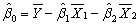
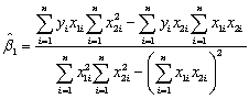
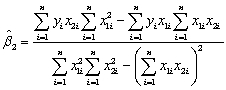
In the multiple regression model with two explanatory variables  the OLS estimators for the three parameters are as follows (small letters refer to deviations from means as in zi = Zi -
  ):
): 
 You have collected data for 104 countries of the world from the Penn World Tables and want to estimate the effect of the population growth rate (
  )and the saving rate (
  )(average investment share of GDP from 1980 to 1990)on GDP per worker (relative to the U.S. )in 1990.The various sums needed to calculate the OLS estimates are given below:
  = 33.33;
  = 2.025;
  = 17.313
  = 8.3103;
  = .0122;
  = 0.6422
  = -0.2304;
  = 1.5676;
  = -0.0520
(a)What are your expected signs for the regression coefficient? Calculate the coefficients and see if their signs correspond to your intuition.
(b)Find the regression ,and interpret it.What other factors can you think of that might have an influence on productivity?
the OLS estimators for the three parameters are as follows (small letters refer to deviations from means as in zi = Zi - ): You have collected data for 104 countries of the world from the Penn World Tables and want to estimate the effect of the population growth rate ( )and the saving rate ( )(average investment share of GDP from 1980 to 1990)on GDP per worker (relative to the U.S. )in 1990.The various sums needed to calculate the OLS estimates are given below: = 33.33; = 2.025; = 17.313 = 8.3103; = .0122; = 0.6422 = -0.2304; = 1.5676; = -0.0520(a)What are your expected signs for the regression coefficient? Calculate the coefficients and see if their signs correspond to your intuition.
(b)Find the regression
,and interpret it.What other factors can you think of that might have an influence on productivity? سؤال
سؤال
In the multiple regression model,the SER is given by
A)
B)
C)
D)
A)
B)
C)
D)
سؤال
Consider the multiple regression model with two regressors X1 and X2,where both variables are determinants of the dependent variable.You first regress Y on X1 only and find no relationship.However when regressing Y on X1 and X2,the slope coefficient  changes by a large amount.This suggests that your first regression suffers from
A)heteroskedasticity
B)perfect multicollinearity
C)omitted variable bias
D)dummy variable trap
changes by a large amount.This suggests that your first regression suffers fromA)heteroskedasticity
B)perfect multicollinearity
C)omitted variable bias
D)dummy variable trap
سؤال
Females,on average,are shorter and weigh less than males.One of your friends,who is a pre-med student,tells you that in addition,females will weigh less for a given height.To test this hypothesis,you collect height and weight of 29 female and 81 male students at your university.A regression of the weight on a constant,height,and a binary variable,which takes a value of one for females and is zero otherwise,yields the following result:  = -229.21 - 6.36 × Female + 5.58 × Height,
  =0.50,SER = 20.99
where Studentw is weight measured in pounds and Height is measured in inches.
(a)Interpret the results.Does it make sense to have a negative intercept?
(b)You decide that in order to give an interpretation to the intercept you should rescale the height variable.One possibility is to subtract 5 ft.or 60 inches from your Height,because the minimum height in your data set is 62 inches.The resulting new intercept is now 105.58.Can you interpret this number now? Do you thing that the regression has changed? What about the standard error of the regression?
(c)You have learned that correlation does not imply causation.Although this is true mathematically,does this always apply?
= -229.21 - 6.36 × Female + 5.58 × Height, =0.50,SER = 20.99where Studentw is weight measured in pounds and Height is measured in inches.
(a)Interpret the results.Does it make sense to have a negative intercept?
(b)You decide that in order to give an interpretation to the intercept you should rescale the height variable.One possibility is to subtract 5 ft.or 60 inches from your Height,because the minimum height in your data set is 62 inches.The resulting new intercept is now 105.58.Can you interpret this number now? Do you thing that the regression
has changed? What about the standard error of the regression?(c)You have learned that correlation does not imply causation.Although this is true mathematically,does this always apply?
سؤال
سؤال
In the multiple regression model Yi = β0 + β1X1i+ β2 X2i + ...+ βkXki + ui,i = 1,... ,n,the OLS estimators are obtained by minimizing the sum of
A)squared mistakes in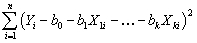
B)squared mistakes in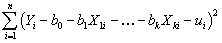
C)absolute mistakes in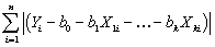
D)squared mistakes in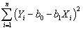
A)squared mistakes in
B)squared mistakes in
C)absolute mistakes in
D)squared mistakes in
سؤال
The Solow growth model suggests that countries with identical saving rates and population growth rates should converge to the same per capita income level.This result has been extended to include investment in human capital (education)as well as investment in physical capital.This hypothesis is referred to as the "conditional convergence hypothesis," since the convergence is dependent on countries obtaining the same values in the driving variables.To test the hypothesis,you collect data from the Penn World Tables on the average annual growth rate of GDP per worker (g6090)for the 1960-1990 sample period,and regress it on the (i)initial starting level of GDP per worker relative to the United States in 1960 (RelProd60), (ii)average population growth rate of the country (n), (iii)average investment share of GDP from 1960 to 1990 (SK - remember investment equals savings),and (iv)educational attainment in years for 1985 (Educ).The results for close to 100 countries is as follows:  = 0.004 - 0.172 × n + 0.133 × SK + 0.002 × Educ - 0.044 × RelProd60,
  =0.537,SER = 0.011
(a)Interpret the results.Do the coefficients have the expected signs? Why does a negative coefficient on the initial level of per capita income indicate conditional convergence ("beta-convergence")?
(b)Equations of the above type have been labeled "determinants of growth" equations in the literature.You recall from your intermediate macroeconomics course that growth in the Solow growth model is determined by technological progress.Yet the above equation does not contain technological progress.Is that inconsistent?
= 0.004 - 0.172 × n + 0.133 × SK + 0.002 × Educ - 0.044 × RelProd60, =0.537,SER = 0.011(a)Interpret the results.Do the coefficients have the expected signs? Why does a negative coefficient on the initial level of per capita income indicate conditional convergence ("beta-convergence")?
(b)Equations of the above type have been labeled "determinants of growth" equations in the literature.You recall from your intermediate macroeconomics course that growth in the Solow growth model is determined by technological progress.Yet the above equation does not contain technological progress.Is that inconsistent?
سؤال
The adjusted R2,or  ,is given by
A)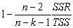
B)
C)
D)
,is given byA)
B)
C)
D)
سؤال
Consider the multiple regression model with two regressors X1 and X2,where both variables are determinants of the dependent variable.When omitting X2 from the regression,then there will be omitted variable bias for 
A)if X1 and X2 are correlated
B)always
C)if X2 is measured in percentages
D)if X2 is a dummy variable
A)if X1 and X2 are correlated
B)always
C)if X2 is measured in percentages
D)if X2 is a dummy variable
سؤال
سؤال
Consider the following multiple regression models (a)to (d)below.DFemme = 1 if the individual is a female,and is zero otherwise;DMale is a binary variable which takes on the value one if the individual is male,and is zero otherwise;DMarried is a binary variable which is unity for married individuals and is zero otherwise,and DSingle is (1-DMarried).Regressing weekly earnings (Earn)on a set of explanatory variables,you will experience perfect multicollinearity in the following cases unless:
A) i =
i =
 +
+
 DFemme +
 Dmale +
 X3i
X3i
B) i =
i =
 +
+
 DMarried +
 DSingle +
 X3i
X3i
C) i =
i =
 +
+
 DFemme +
 X3i
X3i
D) i =
i =
 DFemme +
 Dmale +
 DMarried +
 DSingle +
 X3i
X3i
A)
i = + DFemme + Dmale + X3iB)
i = + DMarried + DSingle + X3iC)
i = + DFemme + X3iD)
i = DFemme + Dmale + DMarried + DSingle + X3i سؤال
سؤال
Attendance at sports events depends on various factors.Teams typically do not change ticket prices from game to game to attract more spectators to less attractive games.However,there are other marketing tools used,such as fireworks,free hats,etc. ,for this purpose.You work as a consultant for a sports team,the Los Angeles Dodgers,to help them forecast attendance,so that they can potentially devise strategies for price discrimination.After collecting data over two years for every one of the 162 home games of the 2000 and 2001 season,you run the following regression:  = 15,005 + 201 × Temperat + 465 × DodgNetWin + 82 × OppNetWin
+ 9647 × DFSaSu + 1328 × Drain + 1609 × D150m + 271 × DDiv - 978 × D2001; =0.416,SER = 6983
where Attend is announced stadium attendance,Temperat it the average temperature on game day,DodgNetWin are the net wins of the Dodgers before the game (wins-losses),OppNetWin is the opposing team's net wins at the end of the previous season,and DFSaSu,Drain,D150m,Ddiv,and D2001 are binary variables,taking a value of 1 if the game was played on a weekend,it rained during that day,the opposing team was within a 150 mile radius,the opposing team plays in the same division as the Dodgers,and the game was played during 2001,respectively.
(a)Interpret the regression results.Do the coefficients have the expected signs?
(b)Excluding the last four binary variables results in the following regression result: = 14,838 + 202 × Temperat + 435 × DodgNetWin + 90 × OppNetWin
+ 10,472 × DFSaSu, =0.410,SER = 6925
According to this regression,what is your forecast of the change in attendance if the temperature increases by 30 degrees? Is it likely that people attend more games if the temperature increases? Is it possible that Temperat picks up the effect of an omitted variable?
(c)Assuming that ticket sales depend on prices,what would your policy advice be for the Dodgers to increase attendance?
(d)Dodger stadium is large and is not often sold out.The Boston Red Sox play in a much smaller stadium,Fenway Park,which often reaches capacity.If you did the same analysis for the Red Sox,what problems would you foresee in your analysis?
= 15,005 + 201 × Temperat + 465 × DodgNetWin + 82 × OppNetWin+ 9647 × DFSaSu + 1328 × Drain + 1609 × D150m + 271 × DDiv - 978 × D2001;
=0.416,SER = 6983where Attend is announced stadium attendance,Temperat it the average temperature on game day,DodgNetWin are the net wins of the Dodgers before the game (wins-losses),OppNetWin is the opposing team's net wins at the end of the previous season,and DFSaSu,Drain,D150m,Ddiv,and D2001 are binary variables,taking a value of 1 if the game was played on a weekend,it rained during that day,the opposing team was within a 150 mile radius,the opposing team plays in the same division as the Dodgers,and the game was played during 2001,respectively.
(a)Interpret the regression results.Do the coefficients have the expected signs?
(b)Excluding the last four binary variables results in the following regression result:
= 14,838 + 202 × Temperat + 435 × DodgNetWin + 90 × OppNetWin+ 10,472 × DFSaSu,
=0.410,SER = 6925According to this regression,what is your forecast of the change in attendance if the temperature increases by 30 degrees? Is it likely that people attend more games if the temperature increases? Is it possible that Temperat picks up the effect of an omitted variable?
(c)Assuming that ticket sales depend on prices,what would your policy advice be for the Dodgers to increase attendance?
(d)Dodger stadium is large and is not often sold out.The Boston Red Sox play in a much smaller stadium,Fenway Park,which often reaches capacity.If you did the same analysis for the Red Sox,what problems would you foresee in your analysis?
سؤال
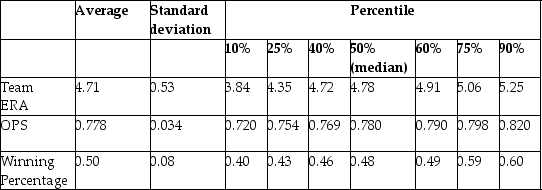
You have collected data from Major League Baseball (MLB)to find the determinants of winning.You have a general idea that both good pitching and strong hitting are needed to do well.However,you do not know how much each of these contributes separately.To investigate this problem,you collect data for all MLB during 1999 season.Your strategy is to first regress the winning percentage on pitching quality ("Team ERA"),second to regress the same variable on some measure of hitting ("OPS - On-base Plus Slugging percentage"),and third to regress the winning percentage on both.
Summary of the Distribution of Winning Percentage,On Base plus Slugging Percentage,
and Team Earned Run Average for MLB in 1999
 The results are as follows:
  = 0.94 - 0.100 × teamera,
  = 0.49,SER = 0.06.
  = -0.68 + 1.513 × ops,
  =0.45,SER = 0.06.
  = -0.19 - 0.099 × teamera + 1.490 × ops,
  =0.92,SER = 0.02.
(a)Interpret the multiple regression.What is the effect of a one point increase in team ERA? Given that the Atlanta Braves had the most wins that year,wining 103 games out of 162,do you find this effect important? Next analyze the importance and statistical significance for the OPS coefficient.(The Minnesota Twins had the minimum OPS of 0.712,while the Texas Rangers had the maximum with 0.840. )Since the intercept is negative,and since winning percentages must lie between zero and one,should you rerun the regression through the origin?
(b)What are some of the omitted variables in your analysis? Are they likely to affect the coefficient on Team ERA and OPS given the size of the and their potential correlation with the included variables?
Summary of the Distribution of Winning Percentage,On Base plus Slugging Percentage,
and Team Earned Run Average for MLB in 1999
The results are as follows: = 0.94 - 0.100 × teamera, = 0.49,SER = 0.06. = -0.68 + 1.513 × ops, =0.45,SER = 0.06. = -0.19 - 0.099 × teamera + 1.490 × ops, =0.92,SER = 0.02.(a)Interpret the multiple regression.What is the effect of a one point increase in team ERA? Given that the Atlanta Braves had the most wins that year,wining 103 games out of 162,do you find this effect important? Next analyze the importance and statistical significance for the OPS coefficient.(The Minnesota Twins had the minimum OPS of 0.712,while the Texas Rangers had the maximum with 0.840. )Since the intercept is negative,and since winning percentages must lie between zero and one,should you rerun the regression through the origin?
(b)What are some of the omitted variables in your analysis? Are they likely to affect the coefficient on Team ERA and OPS given the size of the
and their potential correlation with the included variables? سؤال
In the process of collecting weight and height data from 29 female and 81 male students at your university,you also asked the students for the number of siblings they have.Although it was not quite clear to you initially what you would use that variable for,you construct a new theory that suggests that children who have more siblings come from poorer families and will have to share the food on the table.Although a friend tells you that this theory does not pass the "straight-face" test,you decide to hypothesize that peers with many siblings will weigh less,on average,for a given height.In addition,you believe that the muscle/fat tissue composition of male bodies suggests that females will weigh less,on average,for a given height.To test these theories,you perform the following regression:  = -229.92 - 6.52 × Female + 0.51 × Sibs+ 5.58 × Height,
  =0.50,SER = 21.08
where Studentw is in pounds,Height is in inches,Female takes a value of 1 for females and is 0 otherwise,Sibs is the number of siblings.
Interpret the regression results.
= -229.92 - 6.52 × Female + 0.51 × Sibs+ 5.58 × Height, =0.50,SER = 21.08where Studentw is in pounds,Height is in inches,Female takes a value of 1 for females and is 0 otherwise,Sibs is the number of siblings.
Interpret the regression results.
سؤال
A subsample from the Current Population Survey is taken,on weekly earnings of individuals,their age,and their gender.You have read in the news that women make 70 cents to the $1 that men earn.To test this hypothesis,you first regress earnings on a constant and a binary variable,which takes on a value of 1 for females and is 0 otherwise.The results were:  = 570.70 - 170.72 × Female,
  =0.084,SER = 282.12.
(a)There are 850 females in your sample and 894 males.What are the mean earnings of males and females in this sample? What is the percentage of average female income to male income?
(b)You decide to control for age (in years)in your regression results because older people,up to a point,earn more on average than younger people.This regression output is as follows: = 323.70 - 169.78 × Female + 5.15 × Age,
  =0.135,SER = 274.45.
Interpret these results carefully.How much,on average,does a 40-year-old female make per year in your sample? What about a 20-year-old male? Does this represent stronger evidence of discrimination against females?
= 570.70 - 170.72 × Female, =0.084,SER = 282.12.(a)There are 850 females in your sample and 894 males.What are the mean earnings of males and females in this sample? What is the percentage of average female income to male income?
(b)You decide to control for age (in years)in your regression results because older people,up to a point,earn more on average than younger people.This regression output is as follows:
= 323.70 - 169.78 × Female + 5.15 × Age, =0.135,SER = 274.45.Interpret these results carefully.How much,on average,does a 40-year-old female make per year in your sample? What about a 20-year-old male? Does this represent stronger evidence of discrimination against females?
سؤال
You have collected data for 104 countries to address the difficult questions of the determinants for differences in the standard of living among the countries of the world.You recall from your macroeconomics lectures that the neoclassical growth model suggests that output per worker (per capita income)levels are determined by,among others,the saving rate and population growth rate.To test the predictions of this growth model,you run the following regression:  = 0.339 - 12.894 × n + 1.397 × SK,
  =0.621,SER = 0.177
where RelPersInc is GDP per worker relative to the United States,n is the average population growth rate,1980-1990,and SK is the average investment share of GDP from 1960 to 1990 (remember investment equals saving).
(a)Interpret the results.Do the signs correspond to what you expected them to be? Explain.
(b)You remember that human capital in addition to physical capital also plays a role in determining the standard of living of a country.You therefore collect additional data on the average educational attainment in years for 1985,and add this variable (Educ)to the above regression.This results in the modified regression output: = 0.046 - 5.869 × n + 0.738 × SK + 0.055 × Educ,
  =0.775,SER = 0.1377
How has the inclusion of Educ affected your previous results?
(c)Upon checking the regression output,you realize that there are only 86 observations,since data for Educ is not available for all 104 countries in your sample.Do you have to modify some of your statements in (d)?
(d)Brazil has the following values in your sample: RelPersInc = 0.30,n = 0.021,SK = 0.169,Educ = 3.5.Does your equation overpredict or underpredict the relative GDP per worker? What would happen to this result if Brazil managed to double the average educational attainment?
= 0.339 - 12.894 × n + 1.397 × SK, =0.621,SER = 0.177where RelPersInc is GDP per worker relative to the United States,n is the average population growth rate,1980-1990,and SK is the average investment share of GDP from 1960 to 1990 (remember investment equals saving).
(a)Interpret the results.Do the signs correspond to what you expected them to be? Explain.
(b)You remember that human capital in addition to physical capital also plays a role in determining the standard of living of a country.You therefore collect additional data on the average educational attainment in years for 1985,and add this variable (Educ)to the above regression.This results in the modified regression output:
= 0.046 - 5.869 × n + 0.738 × SK + 0.055 × Educ, =0.775,SER = 0.1377How has the inclusion of Educ affected your previous results?
(c)Upon checking the regression output,you realize that there are only 86 observations,since data for Educ is not available for all 104 countries in your sample.Do you have to modify some of your statements in (d)?
(d)Brazil has the following values in your sample: RelPersInc = 0.30,n = 0.021,SK = 0.169,Educ = 3.5.Does your equation overpredict or underpredict the relative GDP per worker? What would happen to this result if Brazil managed to double the average educational attainment?
سؤال
The cost of attending your college has once again gone up.Although you have been told that education is investment in human capital,which carries a return of roughly 10% a year,you (and your parents)are not pleased.One of the administrators at your university/college does not make the situation better by telling you that you pay more because the reputation of your institution is better than that of others.To investigate this hypothesis,you collect data randomly for 100 national universities and liberal arts colleges from the 2000-2001 U.S.News and World Report annual rankings.Next you perform the following regression  = 7,311.17 + 3,985.20 × Reputation - 0.20 × Size + 8,406.79 × Dpriv - 416.38 × Dlibart - 2,376.51 × Dreligion
R2=0.72,SER = 3,773.35
where Cost is Tuition,Fees,Room and Board in dollars,Reputation is the index used in U.S.News and World Report (based on a survey of university presidents and chief academic officers),which ranges from 1 ("marginal")to 5 ("distinguished"),Size is the number of undergraduate students,and Dpriv,Dlibart,and Dreligion are binary variables indicating whether the institution is private,a liberal arts college,and has a religious affiliation.
(a)Interpret the results.Do the coefficients have the expected sign?
(b)What is the forecasted cost for a liberal arts college,which has no religious affiliation,a size of 1,500 students and a reputation level of 4.5? (All liberal arts colleges are private. )
(c)To save money,you are willing to switch from a private university to a public university,which has a ranking of 0.5 less and 10,000 more students.What is the effect on your cost? Is it substantial?
(d)Eliminating the Size and Dlibart variables from your regression,the estimation regression becomes = 5,450.35 + 3,538.84 × Reputation + 10,935.70 × Dpriv - 2,783.31 × Dreligion;
  =0.72,SER = 3,792.68
Why do you think that the effect of attending a private institution has increased now?
(e)What can you say about causation in the above relationship? Is it possible that Cost affects Reputation rather than the other way around?
= 7,311.17 + 3,985.20 × Reputation - 0.20 × Size + 8,406.79 × Dpriv - 416.38 × Dlibart - 2,376.51 × DreligionR2=0.72,SER = 3,773.35
where Cost is Tuition,Fees,Room and Board in dollars,Reputation is the index used in U.S.News and World Report (based on a survey of university presidents and chief academic officers),which ranges from 1 ("marginal")to 5 ("distinguished"),Size is the number of undergraduate students,and Dpriv,Dlibart,and Dreligion are binary variables indicating whether the institution is private,a liberal arts college,and has a religious affiliation.
(a)Interpret the results.Do the coefficients have the expected sign?
(b)What is the forecasted cost for a liberal arts college,which has no religious affiliation,a size of 1,500 students and a reputation level of 4.5? (All liberal arts colleges are private. )
(c)To save money,you are willing to switch from a private university to a public university,which has a ranking of 0.5 less and 10,000 more students.What is the effect on your cost? Is it substantial?
(d)Eliminating the Size and Dlibart variables from your regression,the estimation regression becomes
= 5,450.35 + 3,538.84 × Reputation + 10,935.70 × Dpriv - 2,783.31 × Dreligion; =0.72,SER = 3,792.68Why do you think that the effect of attending a private institution has increased now?
(e)What can you say about causation in the above relationship? Is it possible that Cost affects Reputation rather than the other way around?
سؤال
The administration of your university/college is thinking about implementing a policy of coed floors only in dormitories.Currently there are only single gender floors.One reason behind such a policy might be to generate an atmosphere of better "understanding" between the sexes.The Dean of Students (DoS)has decided to investigate if such a behavior results in more "togetherness" by attempting to find the determinants of the gender composition at the dinner table in your main dining hall,and in that of a neighboring university,which only allows for coed floors in their dorms.The survey includes 176 students,63 from your university/college,and 113 from a neighboring institution.
(a)The Dean's first problem is how to define gender composition.To begin with,the survey excludes single persons' tables,since the study is to focus on group behavior.The Dean also eliminates sports teams from the analysis,since a large number of single-gender students will sit at the same table.Finally,the Dean decides to only analyze tables with three or more students,since she worries about "couples" distorting the results.The Dean finally settles for the following specification of the dependent variable:
GenderComp= Where "
  " stands for absolute value of Z.The variable can take on values from zero to fifty.Briefly analyze some of the possible values.What are the implications for gender composition as more female students join a given number of males at the table? Why would you choose the absolute value here? Discuss some other possible specifications for the dependent variable.
(b)After considering various explanatory variables,the Dean settles for an initial list of eight,and estimates the following relationship: = 30.90 - 3.78 × Size - 8.81 × DCoed + 2.28 × DFemme + 2.06 × DRoommate
- 0.17 × DAthlete + 1.49 × DCons - 0.81 SAT + 1.74 × SibOther, =0.24,SER = 15.50
where Size is the number of persons at the table minus 3,DCoed is a binary variable,which takes on the value of 1 if you live on a coed floor,DFemme is a binary variable,which is 1 for females and zero otherwise,DRoommate is a binary variable which equals 1 if the person at the table has a roommate and is zero otherwise,DAthlete is a binary variable which is 1 if the person at the table is a member of an athletic varsity team,DCons is a variable which measures the political tendency of the person at the table on a seven-point scale,ranging from 1 being "liberal" to 7 being "conservative," SAT is the SAT score of the person at the table measured on a seven-point scale,ranging from 1 for the category "900-1000" to 7 for the category "1510 and above," and increasing by one for 100 point increases,and SibOther is the number of siblings from the opposite gender in the family the person at the table grew up with.
Interpret the above equation carefully,justifying the inclusion of the explanatory variables along the way.Does it make sense to interpret the constant in the above regression?
(c)Had the Dean used the number of people sitting at the table instead of Number-3,what effect would that have had on the above specification?
(d)If you believe that going down the hallway and knocking on doors is one of the major determinants of who goes to eat with whom,then why would it not be a good idea to survey students at lunch tables?
(a)The Dean's first problem is how to define gender composition.To begin with,the survey excludes single persons' tables,since the study is to focus on group behavior.The Dean also eliminates sports teams from the analysis,since a large number of single-gender students will sit at the same table.Finally,the Dean decides to only analyze tables with three or more students,since she worries about "couples" distorting the results.The Dean finally settles for the following specification of the dependent variable:
GenderComp=
Where " " stands for absolute value of Z.The variable can take on values from zero to fifty.Briefly analyze some of the possible values.What are the implications for gender composition as more female students join a given number of males at the table? Why would you choose the absolute value here? Discuss some other possible specifications for the dependent variable.(b)After considering various explanatory variables,the Dean settles for an initial list of eight,and estimates the following relationship:
= 30.90 - 3.78 × Size - 8.81 × DCoed + 2.28 × DFemme + 2.06 × DRoommate- 0.17 × DAthlete + 1.49 × DCons - 0.81 SAT + 1.74 × SibOther,
=0.24,SER = 15.50where Size is the number of persons at the table minus 3,DCoed is a binary variable,which takes on the value of 1 if you live on a coed floor,DFemme is a binary variable,which is 1 for females and zero otherwise,DRoommate is a binary variable which equals 1 if the person at the table has a roommate and is zero otherwise,DAthlete is a binary variable which is 1 if the person at the table is a member of an athletic varsity team,DCons is a variable which measures the political tendency of the person at the table on a seven-point scale,ranging from 1 being "liberal" to 7 being "conservative," SAT is the SAT score of the person at the table measured on a seven-point scale,ranging from 1 for the category "900-1000" to 7 for the category "1510 and above," and increasing by one for 100 point increases,and SibOther is the number of siblings from the opposite gender in the family the person at the table grew up with.
Interpret the above equation carefully,justifying the inclusion of the explanatory variables along the way.Does it make sense to interpret the constant in the above regression?
(c)Had the Dean used the number of people sitting at the table instead of Number-3,what effect would that have had on the above specification?
(d)If you believe that going down the hallway and knocking on doors is one of the major determinants of who goes to eat with whom,then why would it not be a good idea to survey students at lunch tables?
سؤال
The OLS formula for the slope coefficients in the multiple regression model become increasingly more complicated,using the "sums" expressions,as you add more regressors.For example,in the regression with a single explanatory variable,the formula is 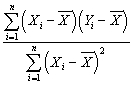 whereas this formula for the slope of the first explanatory variable is
  (small letters refer to deviations from means as in
  )
)
in the case of two explanatory variables.Give an intuitive explanations as to why this is the case.
whereas this formula for the slope of the first explanatory variable is (small letters refer to deviations from means as in )in the case of two explanatory variables.Give an intuitive explanations as to why this is the case.
سؤال
(Requires Statistics background beyond Chapters 2 and 3)One way to establish whether or not there is independence between two or more variables is to perform a  - test on independence between two variables.Explain why multiple regression analysis is a preferable tool to seek a relationship between variables.
- test on independence between two variables.Explain why multiple regression analysis is a preferable tool to seek a relationship between variables. سؤال
سؤال
(Requires Calculus)For the case of the multiple regression problem with two explanatory variables,show that minimizing the sum of squared residuals results in three conditions: 
سؤال
سؤال
In the case of perfect multicollinearity,OLS is unable to calculate the coefficients for the explanatory variables,because it is impossible to change one variable while holding all other variables constant.To see why this is the case,consider the coefficient for the first explanatory variable in the case of a multiple regression model with two explanatory variables:  (small letters refer to deviations from means as in
  ).
).
Divide each of the four terms by to derive an expression in terms of regression coefficients from the simple (one explanatory variable)regression model.In case of perfect multicollinearity,what would be R2 from the regression of
  on
on  ? As a result,what would be the value of the denominator in the above expression for
  ?
?
(small letters refer to deviations from means as in ).Divide each of the four terms by
to derive an expression in terms of regression coefficients from the simple (one explanatory variable)regression model.In case of perfect multicollinearity,what would be R2 from the regression of on ? As a result,what would be the value of the denominator in the above expression for ? سؤال
سؤال
سؤال
(Requires some Calculus)Consider the sample regression function .  .Take the total derivative.Next show that the partial derivative
  is obtained by holding
  constant,or controlling for
  .
.
.Take the total derivative.Next show that the partial derivative is obtained by holding constant,or controlling for . سؤال
You have collected a sub-sample from the Current Population Survey for the western region of the United States.Running a regression of average hourly earnings (ahe)on an intercept only,you get the following result:  =
=  0 = 18.58
a.Interpret the result.
b.You decide to include a single explanatory variable without an intercept.The binary variable DFemme takes on a value of "1" for females but is "0" otherwise.The regression result changes as follows: =
=  1×DFemme = 16.50×DFemme
What is the interpretation now?
c.You generate a new binary variable DMale by subtracting DFemme from 1,and run the new regression: =
=  2×DMale = 20.09×DMale
What is the interpretation of the coefficient now?
d.After thinking about the above results,you recognize that you could have generated the last two results either by running a regression on both binary variables,or on an intercept and one of the binary variables.What would the results have been?
= 0 = 18.58a.Interpret the result.
b.You decide to include a single explanatory variable without an intercept.The binary variable DFemme takes on a value of "1" for females but is "0" otherwise.The regression result changes as follows:
= 1×DFemme = 16.50×DFemmeWhat is the interpretation now?
c.You generate a new binary variable DMale by subtracting DFemme from 1,and run the new regression:
= 2×DMale = 20.09×DMaleWhat is the interpretation of the coefficient now?
d.After thinking about the above results,you recognize that you could have generated the last two results either by running a regression on both binary variables,or on an intercept and one of the binary variables.What would the results have been?
سؤال
It is not hard,but tedious,to derive the OLS formulae for the slope coefficient in the multiple regression case with two explanatory variables.The formula for the first regression slope is 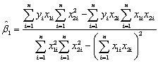 (small letters refer to deviations from means as in
  ).
).
Show that this formula reduces to the slope coefficient for the linear regression model with one regressor if the sample correlation between the two explanatory variables is zero.Given this result,what can you say about the effect of omitting the second explanatory variable from the regression?
(small letters refer to deviations from means as in ).Show that this formula reduces to the slope coefficient for the linear regression model with one regressor if the sample correlation between the two explanatory variables is zero.Given this result,what can you say about the effect of omitting the second explanatory variable from the regression?
سؤال
In the multiple regression problem with k explanatory variable,it would be quite tedious to derive the formulas for the slope coefficients without knowledge of linear algebra.The formulas certainly do not resemble the formula for the slope coefficient in the simple linear regression model with a single explanatory variable.However,it can be shown that the following three step procedure results in the same formula for slope coefficient of the first explanatory variable,  :
:
Step 1: regress Y on a constant and all other explanatory variables other than ,and calculate the residual (Res1).
Step 2: regress on a constant and all other explanatory variables,and calculate the residual (Res2).
Step 3: regress Res1 on a constant and Res2.
Can you give an intuitive explanation to this procedure?
:Step 1: regress Y on a constant and all other explanatory variables other than
,and calculate the residual (Res1).Step 2: regress
on a constant and all other explanatory variables,and calculate the residual (Res2).Step 3: regress Res1 on a constant and Res2.
Can you give an intuitive explanation to this procedure?
سؤال
Your textbook extends the simple regression analysis of Chapters 4 and 5 by adding an additional explanatory variable,the percent of English learners in school districts (PctEl).The results are as follows:  = 698.9 - 2.28 × STR
and = 698.0 - 1.10 × STR - 0.65 × PctEL
Explain why you think the coefficient on the student-teacher ratio has changed so dramatically (been more than halved).
= 698.9 - 2.28 × STRand
= 698.0 - 1.10 × STR - 0.65 × PctELExplain why you think the coefficient on the student-teacher ratio has changed so dramatically (been more than halved).
سؤال
(Requires Calculus)For the simple linear regression model of Chapter 4, 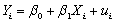 ,the OLS estimator for the intercept was
  ,and
,and 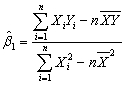 .Intuitively,the OLS estimators for the regression model
 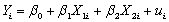 might be
 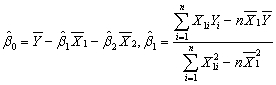 and
and 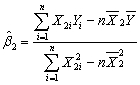 .By minimizing the prediction mistakes of the regression model with two explanatory variables,show that this cannot be the case.
,the OLS estimator for the intercept was ,and .Intuitively,the OLS estimators for the regression model might be and .By minimizing the prediction mistakes of the regression model with two explanatory variables,show that this cannot be the case. سؤال
(Requires Appendix material)Consider the following population regression function model with two explanatory variables:  .It is easy but tedious to show that SE(
  )is given by the following formula:
 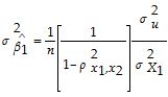 .Sketch how SE(
  )increases with the correlation between
  and
and  .
.
.It is easy but tedious to show that SE( )is given by the following formula: .Sketch how SE( )increases with the correlation between and . سؤال
You have obtained data on test scores and student-teacher ratios in region A and region B of your state.Region B,on average,has lower student-teacher ratios than region A.You decide to run the following regression 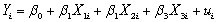 where
where  is the class size in region A,
  is the difference in class size between region A and B,and
  is the class size in region B.Your regression package shows a message indicating that it cannot estimate the above equation.What is the problem here and how can it be fixed?
where is the class size in region A, is the difference in class size between region A and B,and is the class size in region B.Your regression package shows a message indicating that it cannot estimate the above equation.What is the problem here and how can it be fixed? سؤال
سؤال
In the multiple regression model with two regressors,the formula for the slope of the first explanatory variable is  (small letters refer to deviations from means as in
  ).
).
An alternative way to derive the OLS estimator is given through the following three step procedure.
Step 1: regress Y on a constant and ,and calculate the residual (Res1).
Step 2: regress on a constant and
  ,and calculate the residual (Res2).
Step 3: regress Res1 on a constant and Res2.
Prove that the slope of the regression in Step 3 is identical to the above formula.
(small letters refer to deviations from means as in ).An alternative way to derive the OLS estimator is given through the following three step procedure.
Step 1: regress Y on a constant and
,and calculate the residual (Res1).Step 2: regress
on a constant and ,and calculate the residual (Res2).Step 3: regress Res1 on a constant and Res2.
Prove that the slope of the regression in Step 3 is identical to the above formula.
سؤال
سؤال
The probability limit of the OLS estimator in the case of omitted variables is given in your text by the following formula: 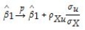 Give an intuitive explanation for two conditions under which the bias will be small.
Give an intuitive explanation for two conditions under which the bias will be small. سؤال
Assume that you have collected cross-sectional data for average hourly earnings (ahe),the number of years of education (educ)and gender of the individuals (you have coded individuals as "1" if they are female and "0" if they are male;the name of the resulting variable is DFemme).
Having faced recent tuition hikes at your university,you are interested in the return to education,that is,how much more will you earn extra for an additional year of being at your institution.To investigate this question,you run the following regression: = -4.58 + 1.71×educ
N = 14,925,R2 = 0.18,SER = 9.30
a.Interpret the regression output.
b.Being a female,you wonder how these results are affected if you entered a binary variable (DFemme),which takes on the value of "1" if the individual is a female,and is "0" for males.The result is as follows: = -3.44 - 4.09×DFemme + 1.76×educ
N = 14,925,R2 = 0.22,SER = 9.08
Does it make sense that the standard error of the regression decreased while the regression R2 increased?
c.Do you think that the regression you estimated first suffered from omitted variable bias?
Having faced recent tuition hikes at your university,you are interested in the return to education,that is,how much more will you earn extra for an additional year of being at your institution.To investigate this question,you run the following regression:
= -4.58 + 1.71×educN = 14,925,R2 = 0.18,SER = 9.30
a.Interpret the regression output.
b.Being a female,you wonder how these results are affected if you entered a binary variable (DFemme),which takes on the value of "1" if the individual is a female,and is "0" for males.The result is as follows:
= -3.44 - 4.09×DFemme + 1.76×educN = 14,925,R2 = 0.22,SER = 9.08
Does it make sense that the standard error of the regression decreased while the regression R2 increased?
c.Do you think that the regression you estimated first suffered from omitted variable bias?
سؤال
سؤال
سؤال
سؤال

فتح الحزمة
قم بالتسجيل لفتح البطاقات في هذه المجموعة!
Unlock Deck
Unlock Deck
1/65
العب
ملء الشاشة (f)
Deck 6: Linear Regression With Multiple Regressors
1
When there are omitted variables in the regression,which are determinants of the dependent variable,then
A)you cannot measure the effect of the omitted variable,but the estimator of your included variable(s)is (are)unaffected.
B)this has no effect on the estimator of your included variable because the other variable is not included.
C)this will always bias the OLS estimator of the included variable.
D)the OLS estimator is biased if the omitted variable is correlated with the included variable.
D
2
The following OLS assumption is most likely violated by omitted variables bias:
A)E(ui Xi)= 0
B)(Xi,Yi)i=1,... ,n are i.i.d draws from their joint distribution
C)there are no outliers for Xi,ui
D)there is heteroskedasticity
A)E(ui
Xi)= 0B)(Xi,Yi)i=1,... ,n are i.i.d draws from their joint distribution
C)there are no outliers for Xi,ui
D)there is heteroskedasticity
A
3
Under imperfect multicollinearity
A)the OLS estimator cannot be computed.
B)two or more of the regressors are highly correlated.
C)the OLS estimator is biased even in samples of n > 100.
D)the error terms are highly,but not perfectly,correlated.
A)the OLS estimator cannot be computed.
B)two or more of the regressors are highly correlated.
C)the OLS estimator is biased even in samples of n > 100.
D)the error terms are highly,but not perfectly,correlated.
B
4
The population multiple regression model when there are two regressors,X1i and X2i can be written as follows,with the exception of:
A)Yi = β0 + β1X1i + β2X2i + ui,i = 1,... ,n
B)Yi = β0X0i + β1X1i + β2X2i + ui,X0i = 1,i = 1,... ,n
C)Yi = Xji + ui,i = 1,... ,n
D)Yi = β0 + β1X1i + β2X2i + ...+ βkXki + ui,i = 1,... ,n
A)Yi = β0 + β1X1i + β2X2i + ui,i = 1,... ,n
B)Yi = β0X0i + β1X1i + β2X2i + ui,X0i = 1,i = 1,... ,n
C)Yi =
Xji + ui,i = 1,... ,nD)Yi = β0 + β1X1i + β2X2i + ...+ βkXki + ui,i = 1,... ,n
فتح الحزمة
افتح القفل للوصول البطاقات البالغ عددها 65 في هذه المجموعة.
فتح الحزمة
k this deck
5
If you had a two regressor regression model,then omitting one variable which is relevant
A)will have no effect on the coefficient of the included variable if the correlation between the excluded and the included variable is negative.
B)will always bias the coefficient of the included variable upwards.
C)can result in a negative value for the coefficient of the included variable,even though the coefficient will have a significant positive effect on Y if the omitted variable were included.
D)makes the sum of the product between the included variable and the residuals different from 0.
فتح الحزمة
افتح القفل للوصول البطاقات البالغ عددها 65 في هذه المجموعة.
فتح الحزمة
k this deck
6
When you have an omitted variable problem,the assumption that E(ui Xi)= 0 is violated.This implies that
A)the sum of the residuals is no longer zero.
B)there is another estimator called weighted least squares,which is BLUE.
C)the sum of the residuals times any of the explanatory variables is no longer zero.
D)the OLS estimator is no longer consistent.
Xi)= 0 is violated.This implies thatA)the sum of the residuals is no longer zero.
B)there is another estimator called weighted least squares,which is BLUE.
C)the sum of the residuals times any of the explanatory variables is no longer zero.
D)the OLS estimator is no longer consistent.
فتح الحزمة
افتح القفل للوصول البطاقات البالغ عددها 65 في هذه المجموعة.
فتح الحزمة
k this deck
7
The intercept in the multiple regression model
A)should be excluded if one explanatory variable has negative values.
B)determines the height of the regression line.
C)should be excluded because the population regression function does not go through the origin.
D)is statistically significant if it is larger than 1.96.
A)should be excluded if one explanatory variable has negative values.
B)determines the height of the regression line.
C)should be excluded because the population regression function does not go through the origin.
D)is statistically significant if it is larger than 1.96.
فتح الحزمة
افتح القفل للوصول البطاقات البالغ عددها 65 في هذه المجموعة.
فتح الحزمة
k this deck
8
In the multiple regression model,the adjusted R2, 2
A)cannot be negative.
B)will never be greater than the regression R2.
C)equals the square of the correlation coefficient r.
D)cannot decrease when an additional explanatory variable is added.
2A)cannot be negative.
B)will never be greater than the regression R2.
C)equals the square of the correlation coefficient r.
D)cannot decrease when an additional explanatory variable is added.
فتح الحزمة
افتح القفل للوصول البطاقات البالغ عددها 65 في هذه المجموعة.
فتح الحزمة
k this deck
9
You have to worry about perfect multicollinearity in the multiple regression model because
A)many economic variables are perfectly correlated.
B)the OLS estimator is no longer BLUE.
C)the OLS estimator cannot be computed in this situation.
D)in real life,economic variables change together all the time.
A)many economic variables are perfectly correlated.
B)the OLS estimator is no longer BLUE.
C)the OLS estimator cannot be computed in this situation.
D)in real life,economic variables change together all the time.
فتح الحزمة
افتح القفل للوصول البطاقات البالغ عددها 65 في هذه المجموعة.
فتح الحزمة
k this deck
10
Imagine you regressed earnings of individuals on a constant,a binary variable ("Male")which takes on the value 1 for males and is 0 otherwise,and another binary variable ("Female")which takes on the value 1 for females and is 0 otherwise.Because females typically earn less than males,you would expect
A)the coefficient for Male to have a positive sign,and for Female a negative sign.
B)both coefficients to be the same distance from the constant,one above and the other below.
C)none of the OLS estimators to exist because there is perfect multicollinearity.
D)this to yield a difference in means statistic.
فتح الحزمة
افتح القفل للوصول البطاقات البالغ عددها 65 في هذه المجموعة.
فتح الحزمة
k this deck
11
(Requires Calculus)In the multiple regression model you estimate the effect on Yi of a unit change in one of the Xi while holding all other regressors constant.This
A)makes little sense,because in the real world all other variables change.
B)corresponds to the economic principle of mutatis mutandis.
C)leaves the formula for the coefficient in the single explanatory variable case unaffected.
D)corresponds to taking a partial derivative in mathematics.
A)makes little sense,because in the real world all other variables change.
B)corresponds to the economic principle of mutatis mutandis.
C)leaves the formula for the coefficient in the single explanatory variable case unaffected.
D)corresponds to taking a partial derivative in mathematics.
فتح الحزمة
افتح القفل للوصول البطاقات البالغ عددها 65 في هذه المجموعة.
فتح الحزمة
k this deck
12
The sample regression line estimated by OLS
A)has an intercept that is equal to zero.
B)is the same as the population regression line.
C)cannot have negative and positive slopes.
D)is the line that minimizes the sum of squared prediction mistakes.
A)has an intercept that is equal to zero.
B)is the same as the population regression line.
C)cannot have negative and positive slopes.
D)is the line that minimizes the sum of squared prediction mistakes.
فتح الحزمة
افتح القفل للوصول البطاقات البالغ عددها 65 في هذه المجموعة.
فتح الحزمة
k this deck
13
Omitted variable bias
A)will always be present as long as the regression R2 < 1.
B)is always there but is negligible in almost all economic examples.
C)exists if the omitted variable is correlated with the included regressor but is not a determinant of the dependent variable.
D)exists if the omitted variable is correlated with the included regressor and is a determinant of the dependent variable.
فتح الحزمة
افتح القفل للوصول البطاقات البالغ عددها 65 في هذه المجموعة.
فتح الحزمة
k this deck
14
In a multiple regression framework,the slope coefficient on the regressor X2i
A)takes into account the scale of the error term.
B)is measured in the units of Yi divided by units of X2i.
C)is usually positive.
D)is larger than the coefficient on X1i.
A)takes into account the scale of the error term.
B)is measured in the units of Yi divided by units of X2i.
C)is usually positive.
D)is larger than the coefficient on X1i.
فتح الحزمة
افتح القفل للوصول البطاقات البالغ عددها 65 في هذه المجموعة.
فتح الحزمة
k this deck
15
In the multiple regression model,the least squares estimator is derived by
A)minimizing the sum of squared prediction mistakes.
B)setting the sum of squared errors equal to zero.
C)minimizing the absolute difference of the residuals.
D)forcing the smallest distance between the actual and fitted values.
A)minimizing the sum of squared prediction mistakes.
B)setting the sum of squared errors equal to zero.
C)minimizing the absolute difference of the residuals.
D)forcing the smallest distance between the actual and fitted values.
فتح الحزمة
افتح القفل للوصول البطاقات البالغ عددها 65 في هذه المجموعة.
فتح الحزمة
k this deck
16
The OLS residuals in the multiple regression model
A)cannot be calculated because there is more than one explanatory variable.
B)can be calculated by subtracting the fitted values from the actual values.
C)are zero because the predicted values are another name for forecasted values.
D)are typically the same as the population regression function errors.
فتح الحزمة
افتح القفل للوصول البطاقات البالغ عددها 65 في هذه المجموعة.
فتح الحزمة
k this deck
17
The main advantage of using multiple regression analysis over differences in means testing is that the regression technique
A)allows you to calculate p-values for the significance of your results.
B)provides you with a measure of your goodness of fit.
C)gives you quantitative estimates of a unit change in X.
D)assumes that the error terms are generated from a normal distribution.
A)allows you to calculate p-values for the significance of your results.
B)provides you with a measure of your goodness of fit.
C)gives you quantitative estimates of a unit change in X.
D)assumes that the error terms are generated from a normal distribution.
فتح الحزمة
افتح القفل للوصول البطاقات البالغ عددها 65 في هذه المجموعة.
فتح الحزمة
k this deck
18
In a two regressor regression model,if you exclude one of the relevant variables then
A)it is no longer reasonable to assume that the errors are homoskedastic.
B)OLS is no longer unbiased,but still consistent.
C)you are no longer controlling for the influence of the other variable.
D)the OLS estimator no longer exists.
A)it is no longer reasonable to assume that the errors are homoskedastic.
B)OLS is no longer unbiased,but still consistent.
C)you are no longer controlling for the influence of the other variable.
D)the OLS estimator no longer exists.
فتح الحزمة
افتح القفل للوصول البطاقات البالغ عددها 65 في هذه المجموعة.
فتح الحزمة
k this deck
19
Under the least squares assumptions for the multiple regression problem (zero conditional mean for the error term,all Xi and Yi being i.i.d. ,all Xi and ui having finite fourth moments,no perfect multicollinearity),the OLS estimators for the slopes and intercept
A)have an exact normal distribution for n > 25.
B)are BLUE.
C)have a normal distribution in small samples as long as the errors are homoskedastic.
D)are unbiased and consistent.
A)have an exact normal distribution for n > 25.
B)are BLUE.
C)have a normal distribution in small samples as long as the errors are homoskedastic.
D)are unbiased and consistent.
فتح الحزمة
افتح القفل للوصول البطاقات البالغ عددها 65 في هذه المجموعة.
فتح الحزمة
k this deck
20
One of the least squares assumptions in the multiple regression model is that you have random variables which are "i.i.d." This stands for
A)initially indeterminate differences.
B)irregularly integrated dichotomies.
C)identically initiated deltas (as in changes).
D)independently and identically distributed.
A)initially indeterminate differences.
B)irregularly integrated dichotomies.
C)identically initiated deltas (as in changes).
D)independently and identically distributed.
فتح الحزمة
افتح القفل للوصول البطاقات البالغ عددها 65 في هذه المجموعة.
فتح الحزمة
k this deck
21
In the multiple regression model with two explanatory variables the OLS estimators for the three parameters are as follows (small letters refer to deviations from means as in zi = Zi - ): You have collected data for 104 countries of the world from the Penn World Tables and want to estimate the effect of the population growth rate ( )and the saving rate ( )(average investment share of GDP from 1980 to 1990)on GDP per worker (relative to the U.S. )in 1990.The various sums needed to calculate the OLS estimates are given below: = 33.33; = 2.025; = 17.313 = 8.3103; = .0122; = 0.6422 = -0.2304; = 1.5676; = -0.0520
(a)What are your expected signs for the regression coefficient? Calculate the coefficients and see if their signs correspond to your intuition.
(b)Find the regression ,and interpret it.What other factors can you think of that might have an influence on productivity?
the OLS estimators for the three parameters are as follows (small letters refer to deviations from means as in zi = Zi - ): You have collected data for 104 countries of the world from the Penn World Tables and want to estimate the effect of the population growth rate ( )and the saving rate ( )(average investment share of GDP from 1980 to 1990)on GDP per worker (relative to the U.S. )in 1990.The various sums needed to calculate the OLS estimates are given below: = 33.33; = 2.025; = 17.313 = 8.3103; = .0122; = 0.6422 = -0.2304; = 1.5676; = -0.0520(a)What are your expected signs for the regression coefficient? Calculate the coefficients and see if their signs correspond to your intuition.
(b)Find the regression
,and interpret it.What other factors can you think of that might have an influence on productivity? فتح الحزمة
افتح القفل للوصول البطاقات البالغ عددها 65 في هذه المجموعة.
فتح الحزمة
k this deck
22
In multiple regression,the R2 increases whenever a regressor is
A)added unless the coefficient on the added regressor is exactly zero.
B)added.
C)added unless there is heterosckedasticity.
D)greater than 1.96 in absolute value.
A)added unless the coefficient on the added regressor is exactly zero.
B)added.
C)added unless there is heterosckedasticity.
D)greater than 1.96 in absolute value.
فتح الحزمة
افتح القفل للوصول البطاقات البالغ عددها 65 في هذه المجموعة.
فتح الحزمة
k this deck
23
In the multiple regression model,the SER is given by
A)
B)
C)
D)
A)
B)
C)
D)
فتح الحزمة
افتح القفل للوصول البطاقات البالغ عددها 65 في هذه المجموعة.
فتح الحزمة
k this deck
24
Consider the multiple regression model with two regressors X1 and X2,where both variables are determinants of the dependent variable.You first regress Y on X1 only and find no relationship.However when regressing Y on X1 and X2,the slope coefficient changes by a large amount.This suggests that your first regression suffers from
A)heteroskedasticity
B)perfect multicollinearity
C)omitted variable bias
D)dummy variable trap
changes by a large amount.This suggests that your first regression suffers fromA)heteroskedasticity
B)perfect multicollinearity
C)omitted variable bias
D)dummy variable trap
فتح الحزمة
افتح القفل للوصول البطاقات البالغ عددها 65 في هذه المجموعة.
فتح الحزمة
k this deck
25
Females,on average,are shorter and weigh less than males.One of your friends,who is a pre-med student,tells you that in addition,females will weigh less for a given height.To test this hypothesis,you collect height and weight of 29 female and 81 male students at your university.A regression of the weight on a constant,height,and a binary variable,which takes a value of one for females and is zero otherwise,yields the following result: = -229.21 - 6.36 × Female + 5.58 × Height, =0.50,SER = 20.99
where Studentw is weight measured in pounds and Height is measured in inches.
(a)Interpret the results.Does it make sense to have a negative intercept?
(b)You decide that in order to give an interpretation to the intercept you should rescale the height variable.One possibility is to subtract 5 ft.or 60 inches from your Height,because the minimum height in your data set is 62 inches.The resulting new intercept is now 105.58.Can you interpret this number now? Do you thing that the regression has changed? What about the standard error of the regression?
(c)You have learned that correlation does not imply causation.Although this is true mathematically,does this always apply?
= -229.21 - 6.36 × Female + 5.58 × Height, =0.50,SER = 20.99where Studentw is weight measured in pounds and Height is measured in inches.
(a)Interpret the results.Does it make sense to have a negative intercept?
(b)You decide that in order to give an interpretation to the intercept you should rescale the height variable.One possibility is to subtract 5 ft.or 60 inches from your Height,because the minimum height in your data set is 62 inches.The resulting new intercept is now 105.58.Can you interpret this number now? Do you thing that the regression
has changed? What about the standard error of the regression?(c)You have learned that correlation does not imply causation.Although this is true mathematically,does this always apply?
فتح الحزمة
افتح القفل للوصول البطاقات البالغ عددها 65 في هذه المجموعة.
فتح الحزمة
k this deck
26
Imperfect multicollinearity
A)is not relevant to the field of economics and business administration
B)only occurs in the study of finance
C)means that the least squares estimator of the slope is biased
D)means that two or more of the regressors are highly correlated
A)is not relevant to the field of economics and business administration
B)only occurs in the study of finance
C)means that the least squares estimator of the slope is biased
D)means that two or more of the regressors are highly correlated
فتح الحزمة
افتح القفل للوصول البطاقات البالغ عددها 65 في هذه المجموعة.
فتح الحزمة
k this deck
27
In the multiple regression model Yi = β0 + β1X1i+ β2 X2i + ...+ βkXki + ui,i = 1,... ,n,the OLS estimators are obtained by minimizing the sum of
A)squared mistakes in
B)squared mistakes in
C)absolute mistakes in
D)squared mistakes in
A)squared mistakes in
B)squared mistakes in
C)absolute mistakes in
D)squared mistakes in
فتح الحزمة
افتح القفل للوصول البطاقات البالغ عددها 65 في هذه المجموعة.
فتح الحزمة
k this deck
28
The Solow growth model suggests that countries with identical saving rates and population growth rates should converge to the same per capita income level.This result has been extended to include investment in human capital (education)as well as investment in physical capital.This hypothesis is referred to as the "conditional convergence hypothesis," since the convergence is dependent on countries obtaining the same values in the driving variables.To test the hypothesis,you collect data from the Penn World Tables on the average annual growth rate of GDP per worker (g6090)for the 1960-1990 sample period,and regress it on the (i)initial starting level of GDP per worker relative to the United States in 1960 (RelProd60), (ii)average population growth rate of the country (n), (iii)average investment share of GDP from 1960 to 1990 (SK - remember investment equals savings),and (iv)educational attainment in years for 1985 (Educ).The results for close to 100 countries is as follows: = 0.004 - 0.172 × n + 0.133 × SK + 0.002 × Educ - 0.044 × RelProd60, =0.537,SER = 0.011
(a)Interpret the results.Do the coefficients have the expected signs? Why does a negative coefficient on the initial level of per capita income indicate conditional convergence ("beta-convergence")?
(b)Equations of the above type have been labeled "determinants of growth" equations in the literature.You recall from your intermediate macroeconomics course that growth in the Solow growth model is determined by technological progress.Yet the above equation does not contain technological progress.Is that inconsistent?
= 0.004 - 0.172 × n + 0.133 × SK + 0.002 × Educ - 0.044 × RelProd60, =0.537,SER = 0.011(a)Interpret the results.Do the coefficients have the expected signs? Why does a negative coefficient on the initial level of per capita income indicate conditional convergence ("beta-convergence")?
(b)Equations of the above type have been labeled "determinants of growth" equations in the literature.You recall from your intermediate macroeconomics course that growth in the Solow growth model is determined by technological progress.Yet the above equation does not contain technological progress.Is that inconsistent?
فتح الحزمة
افتح القفل للوصول البطاقات البالغ عددها 65 في هذه المجموعة.
فتح الحزمة
k this deck
29
The adjusted R2,or ,is given by
A)
B)
C)
D)
,is given byA)
B)
C)
D)
فتح الحزمة
افتح القفل للوصول البطاقات البالغ عددها 65 في هذه المجموعة.
فتح الحزمة
k this deck
30
Consider the multiple regression model with two regressors X1 and X2,where both variables are determinants of the dependent variable.When omitting X2 from the regression,then there will be omitted variable bias for
A)if X1 and X2 are correlated
B)always
C)if X2 is measured in percentages
D)if X2 is a dummy variable
A)if X1 and X2 are correlated
B)always
C)if X2 is measured in percentages
D)if X2 is a dummy variable
فتح الحزمة
افتح القفل للوصول البطاقات البالغ عددها 65 في هذه المجموعة.
فتح الحزمة
k this deck
31
The dummy variable trap is an example of
A)imperfect multicollinearity
B)something that is of theoretical interest only
C)perfect multicollinearity
D)something that does not happen to university or college students
A)imperfect multicollinearity
B)something that is of theoretical interest only
C)perfect multicollinearity
D)something that does not happen to university or college students
فتح الحزمة
افتح القفل للوصول البطاقات البالغ عددها 65 في هذه المجموعة.
فتح الحزمة
k this deck
32
Consider the following multiple regression models (a)to (d)below.DFemme = 1 if the individual is a female,and is zero otherwise;DMale is a binary variable which takes on the value one if the individual is male,and is zero otherwise;DMarried is a binary variable which is unity for married individuals and is zero otherwise,and DSingle is (1-DMarried).Regressing weekly earnings (Earn)on a set of explanatory variables,you will experience perfect multicollinearity in the following cases unless:
A) i =
+
DFemme +
Dmale +
X3i
B) i =
+
DMarried +
DSingle +
X3i
C) i =
+
DFemme +
X3i
D) i =
DFemme +
Dmale +
DMarried +
DSingle +
X3i
A)
i = + DFemme + Dmale + X3iB)
i = + DMarried + DSingle + X3iC)
i = + DFemme + X3iD)
i = DFemme + Dmale + DMarried + DSingle + X3i فتح الحزمة
افتح القفل للوصول البطاقات البالغ عددها 65 في هذه المجموعة.
فتح الحزمة
k this deck
33
Imperfect multicollinearity
A)implies that it will be difficult to estimate precisely one or more of the partial effects using the data at hand
B)violates one of the four Least Squares assumptions in the multiple regression model
C)means that you cannot estimate the effect of at least one of the Xs on Y
D)suggests that a standard spreadsheet program does not have enough power to estimate the multiple regression model
فتح الحزمة
افتح القفل للوصول البطاقات البالغ عددها 65 في هذه المجموعة.
فتح الحزمة
k this deck
34
Attendance at sports events depends on various factors.Teams typically do not change ticket prices from game to game to attract more spectators to less attractive games.However,there are other marketing tools used,such as fireworks,free hats,etc. ,for this purpose.You work as a consultant for a sports team,the Los Angeles Dodgers,to help them forecast attendance,so that they can potentially devise strategies for price discrimination.After collecting data over two years for every one of the 162 home games of the 2000 and 2001 season,you run the following regression: = 15,005 + 201 × Temperat + 465 × DodgNetWin + 82 × OppNetWin
+ 9647 × DFSaSu + 1328 × Drain + 1609 × D150m + 271 × DDiv - 978 × D2001; =0.416,SER = 6983
where Attend is announced stadium attendance,Temperat it the average temperature on game day,DodgNetWin are the net wins of the Dodgers before the game (wins-losses),OppNetWin is the opposing team's net wins at the end of the previous season,and DFSaSu,Drain,D150m,Ddiv,and D2001 are binary variables,taking a value of 1 if the game was played on a weekend,it rained during that day,the opposing team was within a 150 mile radius,the opposing team plays in the same division as the Dodgers,and the game was played during 2001,respectively.
(a)Interpret the regression results.Do the coefficients have the expected signs?
(b)Excluding the last four binary variables results in the following regression result: = 14,838 + 202 × Temperat + 435 × DodgNetWin + 90 × OppNetWin
+ 10,472 × DFSaSu, =0.410,SER = 6925
According to this regression,what is your forecast of the change in attendance if the temperature increases by 30 degrees? Is it likely that people attend more games if the temperature increases? Is it possible that Temperat picks up the effect of an omitted variable?
(c)Assuming that ticket sales depend on prices,what would your policy advice be for the Dodgers to increase attendance?
(d)Dodger stadium is large and is not often sold out.The Boston Red Sox play in a much smaller stadium,Fenway Park,which often reaches capacity.If you did the same analysis for the Red Sox,what problems would you foresee in your analysis?
= 15,005 + 201 × Temperat + 465 × DodgNetWin + 82 × OppNetWin+ 9647 × DFSaSu + 1328 × Drain + 1609 × D150m + 271 × DDiv - 978 × D2001;
=0.416,SER = 6983where Attend is announced stadium attendance,Temperat it the average temperature on game day,DodgNetWin are the net wins of the Dodgers before the game (wins-losses),OppNetWin is the opposing team's net wins at the end of the previous season,and DFSaSu,Drain,D150m,Ddiv,and D2001 are binary variables,taking a value of 1 if the game was played on a weekend,it rained during that day,the opposing team was within a 150 mile radius,the opposing team plays in the same division as the Dodgers,and the game was played during 2001,respectively.
(a)Interpret the regression results.Do the coefficients have the expected signs?
(b)Excluding the last four binary variables results in the following regression result:
= 14,838 + 202 × Temperat + 435 × DodgNetWin + 90 × OppNetWin+ 10,472 × DFSaSu,
=0.410,SER = 6925According to this regression,what is your forecast of the change in attendance if the temperature increases by 30 degrees? Is it likely that people attend more games if the temperature increases? Is it possible that Temperat picks up the effect of an omitted variable?
(c)Assuming that ticket sales depend on prices,what would your policy advice be for the Dodgers to increase attendance?
(d)Dodger stadium is large and is not often sold out.The Boston Red Sox play in a much smaller stadium,Fenway Park,which often reaches capacity.If you did the same analysis for the Red Sox,what problems would you foresee in your analysis?
فتح الحزمة
افتح القفل للوصول البطاقات البالغ عددها 65 في هذه المجموعة.
فتح الحزمة
k this deck
35
You have collected data from Major League Baseball (MLB)to find the determinants of winning.You have a general idea that both good pitching and strong hitting are needed to do well.However,you do not know how much each of these contributes separately.To investigate this problem,you collect data for all MLB during 1999 season.Your strategy is to first regress the winning percentage on pitching quality ("Team ERA"),second to regress the same variable on some measure of hitting ("OPS - On-base Plus Slugging percentage"),and third to regress the winning percentage on both.
Summary of the Distribution of Winning Percentage,On Base plus Slugging Percentage,
and Team Earned Run Average for MLB in 1999
The results are as follows: = 0.94 - 0.100 × teamera, = 0.49,SER = 0.06. = -0.68 + 1.513 × ops, =0.45,SER = 0.06. = -0.19 - 0.099 × teamera + 1.490 × ops, =0.92,SER = 0.02.
(a)Interpret the multiple regression.What is the effect of a one point increase in team ERA? Given that the Atlanta Braves had the most wins that year,wining 103 games out of 162,do you find this effect important? Next analyze the importance and statistical significance for the OPS coefficient.(The Minnesota Twins had the minimum OPS of 0.712,while the Texas Rangers had the maximum with 0.840. )Since the intercept is negative,and since winning percentages must lie between zero and one,should you rerun the regression through the origin?
(b)What are some of the omitted variables in your analysis? Are they likely to affect the coefficient on Team ERA and OPS given the size of the and their potential correlation with the included variables?
Summary of the Distribution of Winning Percentage,On Base plus Slugging Percentage,
and Team Earned Run Average for MLB in 1999
The results are as follows: = 0.94 - 0.100 × teamera, = 0.49,SER = 0.06. = -0.68 + 1.513 × ops, =0.45,SER = 0.06. = -0.19 - 0.099 × teamera + 1.490 × ops, =0.92,SER = 0.02.(a)Interpret the multiple regression.What is the effect of a one point increase in team ERA? Given that the Atlanta Braves had the most wins that year,wining 103 games out of 162,do you find this effect important? Next analyze the importance and statistical significance for the OPS coefficient.(The Minnesota Twins had the minimum OPS of 0.712,while the Texas Rangers had the maximum with 0.840. )Since the intercept is negative,and since winning percentages must lie between zero and one,should you rerun the regression through the origin?
(b)What are some of the omitted variables in your analysis? Are they likely to affect the coefficient on Team ERA and OPS given the size of the
and their potential correlation with the included variables? فتح الحزمة
افتح القفل للوصول البطاقات البالغ عددها 65 في هذه المجموعة.
فتح الحزمة
k this deck
36
In the process of collecting weight and height data from 29 female and 81 male students at your university,you also asked the students for the number of siblings they have.Although it was not quite clear to you initially what you would use that variable for,you construct a new theory that suggests that children who have more siblings come from poorer families and will have to share the food on the table.Although a friend tells you that this theory does not pass the "straight-face" test,you decide to hypothesize that peers with many siblings will weigh less,on average,for a given height.In addition,you believe that the muscle/fat tissue composition of male bodies suggests that females will weigh less,on average,for a given height.To test these theories,you perform the following regression: = -229.92 - 6.52 × Female + 0.51 × Sibs+ 5.58 × Height, =0.50,SER = 21.08
where Studentw is in pounds,Height is in inches,Female takes a value of 1 for females and is 0 otherwise,Sibs is the number of siblings.
Interpret the regression results.
= -229.92 - 6.52 × Female + 0.51 × Sibs+ 5.58 × Height, =0.50,SER = 21.08where Studentw is in pounds,Height is in inches,Female takes a value of 1 for females and is 0 otherwise,Sibs is the number of siblings.
Interpret the regression results.
فتح الحزمة
افتح القفل للوصول البطاقات البالغ عددها 65 في هذه المجموعة.
فتح الحزمة
k this deck
37
A subsample from the Current Population Survey is taken,on weekly earnings of individuals,their age,and their gender.You have read in the news that women make 70 cents to the $1 that men earn.To test this hypothesis,you first regress earnings on a constant and a binary variable,which takes on a value of 1 for females and is 0 otherwise.The results were: = 570.70 - 170.72 × Female, =0.084,SER = 282.12.
(a)There are 850 females in your sample and 894 males.What are the mean earnings of males and females in this sample? What is the percentage of average female income to male income?
(b)You decide to control for age (in years)in your regression results because older people,up to a point,earn more on average than younger people.This regression output is as follows: = 323.70 - 169.78 × Female + 5.15 × Age, =0.135,SER = 274.45.
Interpret these results carefully.How much,on average,does a 40-year-old female make per year in your sample? What about a 20-year-old male? Does this represent stronger evidence of discrimination against females?
= 570.70 - 170.72 × Female, =0.084,SER = 282.12.(a)There are 850 females in your sample and 894 males.What are the mean earnings of males and females in this sample? What is the percentage of average female income to male income?
(b)You decide to control for age (in years)in your regression results because older people,up to a point,earn more on average than younger people.This regression output is as follows:
= 323.70 - 169.78 × Female + 5.15 × Age, =0.135,SER = 274.45.Interpret these results carefully.How much,on average,does a 40-year-old female make per year in your sample? What about a 20-year-old male? Does this represent stronger evidence of discrimination against females?
فتح الحزمة
افتح القفل للوصول البطاقات البالغ عددها 65 في هذه المجموعة.
فتح الحزمة
k this deck
38
You have collected data for 104 countries to address the difficult questions of the determinants for differences in the standard of living among the countries of the world.You recall from your macroeconomics lectures that the neoclassical growth model suggests that output per worker (per capita income)levels are determined by,among others,the saving rate and population growth rate.To test the predictions of this growth model,you run the following regression: = 0.339 - 12.894 × n + 1.397 × SK, =0.621,SER = 0.177
where RelPersInc is GDP per worker relative to the United States,n is the average population growth rate,1980-1990,and SK is the average investment share of GDP from 1960 to 1990 (remember investment equals saving).
(a)Interpret the results.Do the signs correspond to what you expected them to be? Explain.
(b)You remember that human capital in addition to physical capital also plays a role in determining the standard of living of a country.You therefore collect additional data on the average educational attainment in years for 1985,and add this variable (Educ)to the above regression.This results in the modified regression output: = 0.046 - 5.869 × n + 0.738 × SK + 0.055 × Educ, =0.775,SER = 0.1377
How has the inclusion of Educ affected your previous results?
(c)Upon checking the regression output,you realize that there are only 86 observations,since data for Educ is not available for all 104 countries in your sample.Do you have to modify some of your statements in (d)?
(d)Brazil has the following values in your sample: RelPersInc = 0.30,n = 0.021,SK = 0.169,Educ = 3.5.Does your equation overpredict or underpredict the relative GDP per worker? What would happen to this result if Brazil managed to double the average educational attainment?
= 0.339 - 12.894 × n + 1.397 × SK, =0.621,SER = 0.177where RelPersInc is GDP per worker relative to the United States,n is the average population growth rate,1980-1990,and SK is the average investment share of GDP from 1960 to 1990 (remember investment equals saving).
(a)Interpret the results.Do the signs correspond to what you expected them to be? Explain.
(b)You remember that human capital in addition to physical capital also plays a role in determining the standard of living of a country.You therefore collect additional data on the average educational attainment in years for 1985,and add this variable (Educ)to the above regression.This results in the modified regression output:
= 0.046 - 5.869 × n + 0.738 × SK + 0.055 × Educ, =0.775,SER = 0.1377How has the inclusion of Educ affected your previous results?
(c)Upon checking the regression output,you realize that there are only 86 observations,since data for Educ is not available for all 104 countries in your sample.Do you have to modify some of your statements in (d)?
(d)Brazil has the following values in your sample: RelPersInc = 0.30,n = 0.021,SK = 0.169,Educ = 3.5.Does your equation overpredict or underpredict the relative GDP per worker? What would happen to this result if Brazil managed to double the average educational attainment?
فتح الحزمة
افتح القفل للوصول البطاقات البالغ عددها 65 في هذه المجموعة.
فتح الحزمة
k this deck
39
The cost of attending your college has once again gone up.Although you have been told that education is investment in human capital,which carries a return of roughly 10% a year,you (and your parents)are not pleased.One of the administrators at your university/college does not make the situation better by telling you that you pay more because the reputation of your institution is better than that of others.To investigate this hypothesis,you collect data randomly for 100 national universities and liberal arts colleges from the 2000-2001 U.S.News and World Report annual rankings.Next you perform the following regression = 7,311.17 + 3,985.20 × Reputation - 0.20 × Size + 8,406.79 × Dpriv - 416.38 × Dlibart - 2,376.51 × Dreligion
R2=0.72,SER = 3,773.35
where Cost is Tuition,Fees,Room and Board in dollars,Reputation is the index used in U.S.News and World Report (based on a survey of university presidents and chief academic officers),which ranges from 1 ("marginal")to 5 ("distinguished"),Size is the number of undergraduate students,and Dpriv,Dlibart,and Dreligion are binary variables indicating whether the institution is private,a liberal arts college,and has a religious affiliation.
(a)Interpret the results.Do the coefficients have the expected sign?
(b)What is the forecasted cost for a liberal arts college,which has no religious affiliation,a size of 1,500 students and a reputation level of 4.5? (All liberal arts colleges are private. )
(c)To save money,you are willing to switch from a private university to a public university,which has a ranking of 0.5 less and 10,000 more students.What is the effect on your cost? Is it substantial?
(d)Eliminating the Size and Dlibart variables from your regression,the estimation regression becomes = 5,450.35 + 3,538.84 × Reputation + 10,935.70 × Dpriv - 2,783.31 × Dreligion; =0.72,SER = 3,792.68
Why do you think that the effect of attending a private institution has increased now?
(e)What can you say about causation in the above relationship? Is it possible that Cost affects Reputation rather than the other way around?
= 7,311.17 + 3,985.20 × Reputation - 0.20 × Size + 8,406.79 × Dpriv - 416.38 × Dlibart - 2,376.51 × DreligionR2=0.72,SER = 3,773.35
where Cost is Tuition,Fees,Room and Board in dollars,Reputation is the index used in U.S.News and World Report (based on a survey of university presidents and chief academic officers),which ranges from 1 ("marginal")to 5 ("distinguished"),Size is the number of undergraduate students,and Dpriv,Dlibart,and Dreligion are binary variables indicating whether the institution is private,a liberal arts college,and has a religious affiliation.
(a)Interpret the results.Do the coefficients have the expected sign?
(b)What is the forecasted cost for a liberal arts college,which has no religious affiliation,a size of 1,500 students and a reputation level of 4.5? (All liberal arts colleges are private. )
(c)To save money,you are willing to switch from a private university to a public university,which has a ranking of 0.5 less and 10,000 more students.What is the effect on your cost? Is it substantial?
(d)Eliminating the Size and Dlibart variables from your regression,the estimation regression becomes
= 5,450.35 + 3,538.84 × Reputation + 10,935.70 × Dpriv - 2,783.31 × Dreligion; =0.72,SER = 3,792.68Why do you think that the effect of attending a private institution has increased now?
(e)What can you say about causation in the above relationship? Is it possible that Cost affects Reputation rather than the other way around?
فتح الحزمة
افتح القفل للوصول البطاقات البالغ عددها 65 في هذه المجموعة.
فتح الحزمة
k this deck
40
The administration of your university/college is thinking about implementing a policy of coed floors only in dormitories.Currently there are only single gender floors.One reason behind such a policy might be to generate an atmosphere of better "understanding" between the sexes.The Dean of Students (DoS)has decided to investigate if such a behavior results in more "togetherness" by attempting to find the determinants of the gender composition at the dinner table in your main dining hall,and in that of a neighboring university,which only allows for coed floors in their dorms.The survey includes 176 students,63 from your university/college,and 113 from a neighboring institution.
(a)The Dean's first problem is how to define gender composition.To begin with,the survey excludes single persons' tables,since the study is to focus on group behavior.The Dean also eliminates sports teams from the analysis,since a large number of single-gender students will sit at the same table.Finally,the Dean decides to only analyze tables with three or more students,since she worries about "couples" distorting the results.The Dean finally settles for the following specification of the dependent variable:
GenderComp= Where " " stands for absolute value of Z.The variable can take on values from zero to fifty.Briefly analyze some of the possible values.What are the implications for gender composition as more female students join a given number of males at the table? Why would you choose the absolute value here? Discuss some other possible specifications for the dependent variable.
(b)After considering various explanatory variables,the Dean settles for an initial list of eight,and estimates the following relationship: = 30.90 - 3.78 × Size - 8.81 × DCoed + 2.28 × DFemme + 2.06 × DRoommate
- 0.17 × DAthlete + 1.49 × DCons - 0.81 SAT + 1.74 × SibOther, =0.24,SER = 15.50
where Size is the number of persons at the table minus 3,DCoed is a binary variable,which takes on the value of 1 if you live on a coed floor,DFemme is a binary variable,which is 1 for females and zero otherwise,DRoommate is a binary variable which equals 1 if the person at the table has a roommate and is zero otherwise,DAthlete is a binary variable which is 1 if the person at the table is a member of an athletic varsity team,DCons is a variable which measures the political tendency of the person at the table on a seven-point scale,ranging from 1 being "liberal" to 7 being "conservative," SAT is the SAT score of the person at the table measured on a seven-point scale,ranging from 1 for the category "900-1000" to 7 for the category "1510 and above," and increasing by one for 100 point increases,and SibOther is the number of siblings from the opposite gender in the family the person at the table grew up with.
Interpret the above equation carefully,justifying the inclusion of the explanatory variables along the way.Does it make sense to interpret the constant in the above regression?
(c)Had the Dean used the number of people sitting at the table instead of Number-3,what effect would that have had on the above specification?
(d)If you believe that going down the hallway and knocking on doors is one of the major determinants of who goes to eat with whom,then why would it not be a good idea to survey students at lunch tables?
(a)The Dean's first problem is how to define gender composition.To begin with,the survey excludes single persons' tables,since the study is to focus on group behavior.The Dean also eliminates sports teams from the analysis,since a large number of single-gender students will sit at the same table.Finally,the Dean decides to only analyze tables with three or more students,since she worries about "couples" distorting the results.The Dean finally settles for the following specification of the dependent variable:
GenderComp=
Where " " stands for absolute value of Z.The variable can take on values from zero to fifty.Briefly analyze some of the possible values.What are the implications for gender composition as more female students join a given number of males at the table? Why would you choose the absolute value here? Discuss some other possible specifications for the dependent variable.(b)After considering various explanatory variables,the Dean settles for an initial list of eight,and estimates the following relationship:
= 30.90 - 3.78 × Size - 8.81 × DCoed + 2.28 × DFemme + 2.06 × DRoommate- 0.17 × DAthlete + 1.49 × DCons - 0.81 SAT + 1.74 × SibOther,
=0.24,SER = 15.50where Size is the number of persons at the table minus 3,DCoed is a binary variable,which takes on the value of 1 if you live on a coed floor,DFemme is a binary variable,which is 1 for females and zero otherwise,DRoommate is a binary variable which equals 1 if the person at the table has a roommate and is zero otherwise,DAthlete is a binary variable which is 1 if the person at the table is a member of an athletic varsity team,DCons is a variable which measures the political tendency of the person at the table on a seven-point scale,ranging from 1 being "liberal" to 7 being "conservative," SAT is the SAT score of the person at the table measured on a seven-point scale,ranging from 1 for the category "900-1000" to 7 for the category "1510 and above," and increasing by one for 100 point increases,and SibOther is the number of siblings from the opposite gender in the family the person at the table grew up with.
Interpret the above equation carefully,justifying the inclusion of the explanatory variables along the way.Does it make sense to interpret the constant in the above regression?
(c)Had the Dean used the number of people sitting at the table instead of Number-3,what effect would that have had on the above specification?
(d)If you believe that going down the hallway and knocking on doors is one of the major determinants of who goes to eat with whom,then why would it not be a good idea to survey students at lunch tables?
فتح الحزمة
افتح القفل للوصول البطاقات البالغ عددها 65 في هذه المجموعة.
فتح الحزمة
k this deck
41
The OLS formula for the slope coefficients in the multiple regression model become increasingly more complicated,using the "sums" expressions,as you add more regressors.For example,in the regression with a single explanatory variable,the formula is whereas this formula for the slope of the first explanatory variable is (small letters refer to deviations from means as in )
in the case of two explanatory variables.Give an intuitive explanations as to why this is the case.
whereas this formula for the slope of the first explanatory variable is (small letters refer to deviations from means as in )in the case of two explanatory variables.Give an intuitive explanations as to why this is the case.
فتح الحزمة
افتح القفل للوصول البطاقات البالغ عددها 65 في هذه المجموعة.
فتح الحزمة
k this deck
42
(Requires Statistics background beyond Chapters 2 and 3)One way to establish whether or not there is independence between two or more variables is to perform a - test on independence between two variables.Explain why multiple regression analysis is a preferable tool to seek a relationship between variables.
- test on independence between two variables.Explain why multiple regression analysis is a preferable tool to seek a relationship between variables. فتح الحزمة
افتح القفل للوصول البطاقات البالغ عددها 65 في هذه المجموعة.
فتح الحزمة
k this deck
43
In the multiple regression with two explanatory variables,show that the TSS can still be decomposed into the ESS and the RSS.
فتح الحزمة
افتح القفل للوصول البطاقات البالغ عددها 65 في هذه المجموعة.
فتح الحزمة
k this deck
44
(Requires Calculus)For the case of the multiple regression problem with two explanatory variables,show that minimizing the sum of squared residuals results in three conditions:
فتح الحزمة
افتح القفل للوصول البطاقات البالغ عددها 65 في هذه المجموعة.
فتح الحزمة
k this deck
45
You try to establish that there is a positive relationship between the use of a fertilizer and the growth of a certain plant.Set up the design of an experiment to establish the relationship,paying particular attention to relevant control variables.Discuss in this context the effect of omitted variable bias.
فتح الحزمة
افتح القفل للوصول البطاقات البالغ عددها 65 في هذه المجموعة.
فتح الحزمة
k this deck
46
In the case of perfect multicollinearity,OLS is unable to calculate the coefficients for the explanatory variables,because it is impossible to change one variable while holding all other variables constant.To see why this is the case,consider the coefficient for the first explanatory variable in the case of a multiple regression model with two explanatory variables: (small letters refer to deviations from means as in ).
Divide each of the four terms by to derive an expression in terms of regression coefficients from the simple (one explanatory variable)regression model.In case of perfect multicollinearity,what would be R2 from the regression of on ? As a result,what would be the value of the denominator in the above expression for ?
(small letters refer to deviations from means as in ).Divide each of the four terms by
to derive an expression in terms of regression coefficients from the simple (one explanatory variable)regression model.In case of perfect multicollinearity,what would be R2 from the regression of on ? As a result,what would be the value of the denominator in the above expression for ? فتح الحزمة
افتح القفل للوصول البطاقات البالغ عددها 65 في هذه المجموعة.
فتح الحزمة
k this deck
47
Give at least three examples from macroeconomics and three from microeconomics that involve specified equations in a multiple regression analysis framework.Indicate in each case what the expected signs of the coefficients would be and if theory gives you an indication about the likely size of the coefficients.
فتح الحزمة
افتح القفل للوصول البطاقات البالغ عددها 65 في هذه المجموعة.
فتح الحزمة
k this deck
48
Your econometrics textbook stated that there will be omitted variable bias in the OLS estimator unless the included regressor,X,is uncorrelated with the omitted variable or the omitted variable is not a determinant of the dependent variable,Y.Give an intuitive explanation for these two conditions.
فتح الحزمة
افتح القفل للوصول البطاقات البالغ عددها 65 في هذه المجموعة.
فتح الحزمة
k this deck
49
(Requires some Calculus)Consider the sample regression function . .Take the total derivative.Next show that the partial derivative is obtained by holding constant,or controlling for .
.Take the total derivative.Next show that the partial derivative is obtained by holding constant,or controlling for . فتح الحزمة
افتح القفل للوصول البطاقات البالغ عددها 65 في هذه المجموعة.
فتح الحزمة
k this deck
50
You have collected a sub-sample from the Current Population Survey for the western region of the United States.Running a regression of average hourly earnings (ahe)on an intercept only,you get the following result: = 0 = 18.58
a.Interpret the result.
b.You decide to include a single explanatory variable without an intercept.The binary variable DFemme takes on a value of "1" for females but is "0" otherwise.The regression result changes as follows: = 1×DFemme = 16.50×DFemme
What is the interpretation now?
c.You generate a new binary variable DMale by subtracting DFemme from 1,and run the new regression: = 2×DMale = 20.09×DMale
What is the interpretation of the coefficient now?
d.After thinking about the above results,you recognize that you could have generated the last two results either by running a regression on both binary variables,or on an intercept and one of the binary variables.What would the results have been?
= 0 = 18.58a.Interpret the result.
b.You decide to include a single explanatory variable without an intercept.The binary variable DFemme takes on a value of "1" for females but is "0" otherwise.The regression result changes as follows:
= 1×DFemme = 16.50×DFemmeWhat is the interpretation now?
c.You generate a new binary variable DMale by subtracting DFemme from 1,and run the new regression:
= 2×DMale = 20.09×DMaleWhat is the interpretation of the coefficient now?
d.After thinking about the above results,you recognize that you could have generated the last two results either by running a regression on both binary variables,or on an intercept and one of the binary variables.What would the results have been?
فتح الحزمة
افتح القفل للوصول البطاقات البالغ عددها 65 في هذه المجموعة.
فتح الحزمة
k this deck
51
It is not hard,but tedious,to derive the OLS formulae for the slope coefficient in the multiple regression case with two explanatory variables.The formula for the first regression slope is (small letters refer to deviations from means as in ).
Show that this formula reduces to the slope coefficient for the linear regression model with one regressor if the sample correlation between the two explanatory variables is zero.Given this result,what can you say about the effect of omitting the second explanatory variable from the regression?
(small letters refer to deviations from means as in ).Show that this formula reduces to the slope coefficient for the linear regression model with one regressor if the sample correlation between the two explanatory variables is zero.Given this result,what can you say about the effect of omitting the second explanatory variable from the regression?
فتح الحزمة
افتح القفل للوصول البطاقات البالغ عددها 65 في هذه المجموعة.
فتح الحزمة
k this deck
52
In the multiple regression problem with k explanatory variable,it would be quite tedious to derive the formulas for the slope coefficients without knowledge of linear algebra.The formulas certainly do not resemble the formula for the slope coefficient in the simple linear regression model with a single explanatory variable.However,it can be shown that the following three step procedure results in the same formula for slope coefficient of the first explanatory variable, :
Step 1: regress Y on a constant and all other explanatory variables other than ,and calculate the residual (Res1).
Step 2: regress on a constant and all other explanatory variables,and calculate the residual (Res2).
Step 3: regress Res1 on a constant and Res2.
Can you give an intuitive explanation to this procedure?
:Step 1: regress Y on a constant and all other explanatory variables other than
,and calculate the residual (Res1).Step 2: regress
on a constant and all other explanatory variables,and calculate the residual (Res2).Step 3: regress Res1 on a constant and Res2.
Can you give an intuitive explanation to this procedure?
فتح الحزمة
افتح القفل للوصول البطاقات البالغ عددها 65 في هذه المجموعة.
فتح الحزمة
k this deck
53
Your textbook extends the simple regression analysis of Chapters 4 and 5 by adding an additional explanatory variable,the percent of English learners in school districts (PctEl).The results are as follows: = 698.9 - 2.28 × STR
and = 698.0 - 1.10 × STR - 0.65 × PctEL
Explain why you think the coefficient on the student-teacher ratio has changed so dramatically (been more than halved).
= 698.9 - 2.28 × STRand
= 698.0 - 1.10 × STR - 0.65 × PctELExplain why you think the coefficient on the student-teacher ratio has changed so dramatically (been more than halved).
فتح الحزمة
افتح القفل للوصول البطاقات البالغ عددها 65 في هذه المجموعة.
فتح الحزمة
k this deck
54
(Requires Calculus)For the simple linear regression model of Chapter 4, ,the OLS estimator for the intercept was ,and .Intuitively,the OLS estimators for the regression model might be and .By minimizing the prediction mistakes of the regression model with two explanatory variables,show that this cannot be the case.
,the OLS estimator for the intercept was ,and .Intuitively,the OLS estimators for the regression model might be and .By minimizing the prediction mistakes of the regression model with two explanatory variables,show that this cannot be the case. فتح الحزمة
افتح القفل للوصول البطاقات البالغ عددها 65 في هذه المجموعة.
فتح الحزمة
k this deck
55
(Requires Appendix material)Consider the following population regression function model with two explanatory variables: .It is easy but tedious to show that SE( )is given by the following formula: .Sketch how SE( )increases with the correlation between and .
.It is easy but tedious to show that SE( )is given by the following formula: .Sketch how SE( )increases with the correlation between and . فتح الحزمة
افتح القفل للوصول البطاقات البالغ عددها 65 في هذه المجموعة.
فتح الحزمة
k this deck
56
You have obtained data on test scores and student-teacher ratios in region A and region B of your state.Region B,on average,has lower student-teacher ratios than region A.You decide to run the following regression where is the class size in region A, is the difference in class size between region A and B,and is the class size in region B.Your regression package shows a message indicating that it cannot estimate the above equation.What is the problem here and how can it be fixed?
where is the class size in region A, is the difference in class size between region A and B,and is the class size in region B.Your regression package shows a message indicating that it cannot estimate the above equation.What is the problem here and how can it be fixed? فتح الحزمة
افتح القفل للوصول البطاقات البالغ عددها 65 في هذه المجموعة.
فتح الحزمة
k this deck
57
(Requires Calculus)For the case of the multiple regression problem with two explanatory variables,derive the OLS estimator for the intercept and the two slopes.
فتح الحزمة
افتح القفل للوصول البطاقات البالغ عددها 65 في هذه المجموعة.
فتح الحزمة
k this deck
58
In the multiple regression model with two regressors,the formula for the slope of the first explanatory variable is (small letters refer to deviations from means as in ).
An alternative way to derive the OLS estimator is given through the following three step procedure.
Step 1: regress Y on a constant and ,and calculate the residual (Res1).
Step 2: regress on a constant and ,and calculate the residual (Res2).
Step 3: regress Res1 on a constant and Res2.
Prove that the slope of the regression in Step 3 is identical to the above formula.
(small letters refer to deviations from means as in ).An alternative way to derive the OLS estimator is given through the following three step procedure.
Step 1: regress Y on a constant and
,and calculate the residual (Res1).Step 2: regress
on a constant and ,and calculate the residual (Res2).Step 3: regress Res1 on a constant and Res2.
Prove that the slope of the regression in Step 3 is identical to the above formula.
فتح الحزمة
افتح القفل للوصول البطاقات البالغ عددها 65 في هذه المجموعة.
فتح الحزمة
k this deck
59
One of your peers wants to analyze whether or not participating in varsity sports lowers or increases the GPA of students.She decides to collect data from 110 male and female students on their GPA and the number of hours they spend participating in varsity sports.The coefficient in the simple regression function turns out to be significantly negative,using the t-statistic and carrying out the appropriate hypothesis test.Upon reflection,she is concerned that she did not ask the students in her sample whether or not they were female or male.You point out to her that you are more concerned about the effect of omitted variables in her regression,such as the incoming SAT score of the students,and whether or not they are in a major from a high/low grading department.Elaborate on your argument.
فتح الحزمة
افتح القفل للوصول البطاقات البالغ عددها 65 في هذه المجموعة.
فتح الحزمة
k this deck
60
The probability limit of the OLS estimator in the case of omitted variables is given in your text by the following formula: Give an intuitive explanation for two conditions under which the bias will be small.
Give an intuitive explanation for two conditions under which the bias will be small. فتح الحزمة
افتح القفل للوصول البطاقات البالغ عددها 65 في هذه المجموعة.
فتح الحزمة
k this deck
61
Assume that you have collected cross-sectional data for average hourly earnings (ahe),the number of years of education (educ)and gender of the individuals (you have coded individuals as "1" if they are female and "0" if they are male;the name of the resulting variable is DFemme).
Having faced recent tuition hikes at your university,you are interested in the return to education,that is,how much more will you earn extra for an additional year of being at your institution.To investigate this question,you run the following regression: = -4.58 + 1.71×educ
N = 14,925,R2 = 0.18,SER = 9.30
a.Interpret the regression output.
b.Being a female,you wonder how these results are affected if you entered a binary variable (DFemme),which takes on the value of "1" if the individual is a female,and is "0" for males.The result is as follows: = -3.44 - 4.09×DFemme + 1.76×educ
N = 14,925,R2 = 0.22,SER = 9.08
Does it make sense that the standard error of the regression decreased while the regression R2 increased?
c.Do you think that the regression you estimated first suffered from omitted variable bias?
Having faced recent tuition hikes at your university,you are interested in the return to education,that is,how much more will you earn extra for an additional year of being at your institution.To investigate this question,you run the following regression:
= -4.58 + 1.71×educN = 14,925,R2 = 0.18,SER = 9.30
a.Interpret the regression output.
b.Being a female,you wonder how these results are affected if you entered a binary variable (DFemme),which takes on the value of "1" if the individual is a female,and is "0" for males.The result is as follows:
= -3.44 - 4.09×DFemme + 1.76×educN = 14,925,R2 = 0.22,SER = 9.08
Does it make sense that the standard error of the regression decreased while the regression R2 increased?
c.Do you think that the regression you estimated first suffered from omitted variable bias?
فتح الحزمة
افتح القفل للوصول البطاقات البالغ عددها 65 في هذه المجموعة.
فتح الحزمة
k this deck
62
You would like to find the effect of gender and marital status on earnings.As a result,you consider running the following regression:
ahei= β0 + β1×DFemmei + β2×DMarri + β3×DSinglei + β4×educi+...+ ui
Where ahe is average hourly earnings,DFemme is a binary variable which takes on the value of "1" if the individual is a female and is "0" otherwise,DMarr is a binary variable which takes on the value of "1" if the individual is married and is "0" otherwise,DSingle takes on the value of "1" if the individual is not married and is "0" otherwise.The regression program which you are using either returns a message that the equation cannot be estimated or drops one of the coefficients.Why do you think that is?
فتح الحزمة
افتح القفل للوصول البطاقات البالغ عددها 65 في هذه المجموعة.
فتح الحزمة
k this deck
63
Consider the following earnings function:
ahei= β0 + β1×DFemmei + β2×educi+...+ ui
versus the alternative specification
ahei= γ0 × DMale + γ1×DFemmei + γ2×educi+...+ ui
where ahe is average hourly earnings,DFemme is a binary variable which takes on the value of "1" if the individual is a female and is "0" otherwise,educ measures the years of education,and DMale is a binary variable which takes on the value of "1" if the individual is a male and is "0" otherwise.There may be additional explanatory variables in the equation.
a.How do the βs and γs compare? Putting it differently,having estimated the coefficients in the first equation,can you derive the coefficients in the second equation without re-estimating the regression?
b.Will the goodness of fit measures,such as the regression R2,differ between the two equations?
c.What is the reason why economists typically prefer the second specification over the first?
فتح الحزمة
افتح القفل للوصول البطاقات البالغ عددها 65 في هذه المجموعة.
فتح الحزمة
k this deck
64
For this question,use the California Testscore Data Set and your regression package (a spreadsheet program if necessary).First perform a multiple regression of testscores on a constant,the student-teacher ratio,and the percent of English learners.Record the coefficients.Next,do the following three step procedure instead: first,regress the testscore on a constant and the percent of English learners.Calculate the residuals and store them under the name resYX2.Second,regress the student-teacher ratio on a constant and the percent of English learners.Calculate the residuals from this regression and store these under the name resX1X2.Finally regress resYX2 on resX1X2 (and a constant,if you wish).Explain intuitively why the simple regression coefficient in the last regression is identical to the regression coefficient on the student-teacher ratio in the multiple regression.
فتح الحزمة
افتح القفل للوصول البطاقات البالغ عددها 65 في هذه المجموعة.
فتح الحزمة
k this deck
65
You have collected data on individuals and their attributes.Consequently you have generated several binary variables,which take on a value of "1" if the individual has that characteristic and are "0" otherwise.One example is the binary variable DMarr which is "1" for married individuals and "0" for non-married variables.If you run the following regression:
ahei= β0 + β1×educi + β2×DMarri + ui
a.What is the interpretation for β2?
b.You are interested in directly observing the effect that being non-married ("single")has on earnings,controlling for years of education.Instead of recording all observations such that they are "1" for a not married individual and "0" for a married person,how can you generate such a variable (DSingle)through a simple command in your regression program?
فتح الحزمة
افتح القفل للوصول البطاقات البالغ عددها 65 في هذه المجموعة.
فتح الحزمة
k this deck
فتح الحزمة
افتح القفل للوصول البطاقات البالغ عددها 65 في هذه المجموعة.


