Deck 16: Additional Topics in Time Series Regression
ملء الشاشة (f)
سؤال
سؤال
سؤال
سؤال
سؤال
سؤال
سؤال
سؤال
سؤال
سؤال
سؤال
سؤال
سؤال
سؤال
سؤال
Δ2Yt
A)= ΔYt - ΔYt-1.
B)= -
-
 .
.
C)= ΔYt -ΔYt-2.
D)= Yt - Yt-2.
A)= ΔYt - ΔYt-1.
B)=
- .C)= ΔYt -ΔYt-2.
D)= Yt - Yt-2.
سؤال
سؤال
سؤال
سؤال
سؤال
سؤال
You have collected quarterly data on inflation and unemployment rates for Canada from 1961:III to 1995:IV to estimate a VAR(4)model of the change in the rate of inflation and the unemployment rate.The results are  t = 1.02 - .54 ΔInft-1 - .46 ΔInft-2 - .32 ΔInft-2 - .01 ΔInft-4
.09)(.09)(.09)(.08)(.44)
-.76 Unempt-1 + .20 Unempt-2 - .16 Unempt-3 + .59 Unempt-4
(.43)(.76)(.76)(.44) = .26.
  t = 0.18 - .003 ΔInft-1 - .016 ΔInft-2 - .018 ΔInft-3 - .010 ΔInft-4
(.10)(.016)(.018)(.017)(.016)
+ 1.47 Unempt-1 - .46 Unempt-2 - .08 Unempt-3 + .05 Unempt-4
(.08)(.14)(.14)(.08) = .980.
(a)Explain how you would use the above regressions to conduct one period ahead forecasts.
(b)Should you test for cointegration between the change in the inflation rate and the unemployment rate and,in the case of finding cointegration here,respecify the above model as a VECM?
(c)The Granger causality test yields the following F-statistics: 3.75 for the test that the coefficients on lagged unemployment rate in the change of inflation equation are all zero;and 0.36 for the test that the coefficients on lagged changes in the inflation rate are all zero.Based on these results,does unemployment Granger-cause inflation? Does inflation Granger-cause unemployment?
t = 1.02 - .54 ΔInft-1 - .46 ΔInft-2 - .32 ΔInft-2 - .01 ΔInft-4.09)(.09)(.09)(.08)(.44)
-.76 Unempt-1 + .20 Unempt-2 - .16 Unempt-3 + .59 Unempt-4
(.43)(.76)(.76)(.44)
= .26. t = 0.18 - .003 ΔInft-1 - .016 ΔInft-2 - .018 ΔInft-3 - .010 ΔInft-4(.10)(.016)(.018)(.017)(.016)
+ 1.47 Unempt-1 - .46 Unempt-2 - .08 Unempt-3 + .05 Unempt-4
(.08)(.14)(.14)(.08)
= .980.(a)Explain how you would use the above regressions to conduct one period ahead forecasts.
(b)Should you test for cointegration between the change in the inflation rate and the unemployment rate and,in the case of finding cointegration here,respecify the above model as a VECM?
(c)The Granger causality test yields the following F-statistics: 3.75 for the test that the coefficients on lagged unemployment rate in the change of inflation equation are all zero;and 0.36 for the test that the coefficients on lagged changes in the inflation rate are all zero.Based on these results,does unemployment Granger-cause inflation? Does inflation Granger-cause unemployment?
سؤال
You have collected quarterly data for the unemployment rate (Unemp)in the United States,using a sample period from 1962:I (first quarter)to 2009:IV (the data is collected at a monthly frequency,but you have taken quarterly averages).
a.Does economic theory suggest that the unemployment rate should be stationary?
b.Testing the unemployment rate for stationarity,you run the following regression (where the lag length was determined using the BIC;using the AIC instead does not change the outcome of the test,even though it chooses 9 lags of the LHS variable): t = 0.217 - 0.035 Unempt-1 + 0.689 ΔUnempt-1
(0.01)0.0012)(0.054)
Use the ADF statistic with an intercept only to test for stationarity.What is your decision?
c.The standard errors reported above were homoskedasticity-only standard errors.Do you think you could potentially improve on inference by allowing for HAC standard errors?
d.An alternative test for a unit root,the DF-GLS,produces a test statistic of -2.75.Find the critical value and decide whether or not to reject the null hypothesis.If the decision is different from (c),is there any reason why you might prefer the DF-GLS test over the ADF test?
a.Does economic theory suggest that the unemployment rate should be stationary?
b.Testing the unemployment rate for stationarity,you run the following regression (where the lag length was determined using the BIC;using the AIC instead does not change the outcome of the test,even though it chooses 9 lags of the LHS variable):
t = 0.217 - 0.035 Unempt-1 + 0.689 ΔUnempt-1(0.01)0.0012)(0.054)
Use the ADF statistic with an intercept only to test for stationarity.What is your decision?
c.The standard errors reported above were homoskedasticity-only standard errors.Do you think you could potentially improve on inference by allowing for HAC standard errors?
d.An alternative test for a unit root,the DF-GLS,produces a test statistic of -2.75.Find the critical value and decide whether or not to reject the null hypothesis.If the decision is different from (c),is there any reason why you might prefer the DF-GLS test over the ADF test?
سؤال
سؤال
سؤال
سؤال
Using the ADL(1,1)regression Yt = β0 + β1Yt-1 +  Xt-1 + ut,the ARCH model for the regression error assumes that ut is normally distributed with mean zero and variance
  ,where
A) = α0 + α1
 + α2
+ α2
 + ...+ αp
 .
.
B) =
=
 + ...+
 + φ1
+ φ1
 + ...+ φq
 .
.
C) = φ1
= φ1
 + ...+ φq
 .
.
D) = α0 + α1
 + ...+ αp
 + φ1
+ φ1
 + ...+ φq
 .
.
Xt-1 + ut,the ARCH model for the regression error assumes that ut is normally distributed with mean zero and variance ,whereA)
= α0 + α1 + α2 + ...+ αp .B)
= + ...+ + φ1 + ...+ φq .C)
= φ1 + ...+ φq .D)
= α0 + α1 + ...+ αp + φ1 + ...+ φq . سؤال
سؤال
The BIC for the VAR is
A)BIC(p)= ln[det (![<strong>The BIC for the VAR is</strong> A)BIC(p)= ln[det ( u)] + k(kp+1) B)BIC(p)= ln[det ( u)] + k(p+1) C)BIC(p)= ln[det ( u)] + k(kp+1) D)BIC(p)= ln[SSR(p)] + k(p+1) <div style=padding-top: 35px>](https://d2lvgg3v3hfg70.cloudfront.net/TB2833/11eab146_bd62_ff1b_896a_e1956f793bbd_TB2833_11.jpg) u)] + k(kp+1)
u)] + k(kp+1)
![<strong>The BIC for the VAR is</strong> A)BIC(p)= ln[det ( u)] + k(kp+1) B)BIC(p)= ln[det ( u)] + k(p+1) C)BIC(p)= ln[det ( u)] + k(kp+1) D)BIC(p)= ln[SSR(p)] + k(p+1) <div style=padding-top: 35px>](https://d2lvgg3v3hfg70.cloudfront.net/TB2833/11eab146_bd62_ff1c_896a_9fdca345c250_TB2833_11.jpg)
B)BIC(p)= ln[det (![<strong>The BIC for the VAR is</strong> A)BIC(p)= ln[det ( u)] + k(kp+1) B)BIC(p)= ln[det ( u)] + k(p+1) C)BIC(p)= ln[det ( u)] + k(kp+1) D)BIC(p)= ln[SSR(p)] + k(p+1) <div style=padding-top: 35px>](https://d2lvgg3v3hfg70.cloudfront.net/TB2833/11eab146_bd63_262d_896a_db6f42765b95_TB2833_11.jpg) u)] + k(p+1)
u)] + k(p+1)
![<strong>The BIC for the VAR is</strong> A)BIC(p)= ln[det ( u)] + k(kp+1) B)BIC(p)= ln[det ( u)] + k(p+1) C)BIC(p)= ln[det ( u)] + k(kp+1) D)BIC(p)= ln[SSR(p)] + k(p+1) <div style=padding-top: 35px>](https://d2lvgg3v3hfg70.cloudfront.net/TB2833/11eab146_bd63_262e_896a_37d52af63c3a_TB2833_11.jpg)
C)BIC(p)= ln[det (![<strong>The BIC for the VAR is</strong> A)BIC(p)= ln[det ( u)] + k(kp+1) B)BIC(p)= ln[det ( u)] + k(p+1) C)BIC(p)= ln[det ( u)] + k(kp+1) D)BIC(p)= ln[SSR(p)] + k(p+1) <div style=padding-top: 35px>](https://d2lvgg3v3hfg70.cloudfront.net/TB2833/11eab146_bd63_262f_896a_dd9048647063_TB2833_00.jpg) u)] + k(kp+1)
u)] + k(kp+1)
![<strong>The BIC for the VAR is</strong> A)BIC(p)= ln[det ( u)] + k(kp+1) B)BIC(p)= ln[det ( u)] + k(p+1) C)BIC(p)= ln[det ( u)] + k(kp+1) D)BIC(p)= ln[SSR(p)] + k(p+1) <div style=padding-top: 35px>](https://d2lvgg3v3hfg70.cloudfront.net/TB2833/11eab146_bd63_2630_896a_fdd9975791e9_TB2833_11.jpg)
D)BIC(p)= ln[SSR(p)] + k(p+1)![<strong>The BIC for the VAR is</strong> A)BIC(p)= ln[det ( u)] + k(kp+1) B)BIC(p)= ln[det ( u)] + k(p+1) C)BIC(p)= ln[det ( u)] + k(kp+1) D)BIC(p)= ln[SSR(p)] + k(p+1) <div style=padding-top: 35px>](https://d2lvgg3v3hfg70.cloudfront.net/TB2833/11eab146_bd63_2631_896a_2906a9a38d93_TB2833_11.jpg)
A)BIC(p)= ln[det (
u)] + k(kp+1)B)BIC(p)= ln[det (
u)] + k(p+1)C)BIC(p)= ln[det (
u)] + k(kp+1)D)BIC(p)= ln[SSR(p)] + k(p+1)
سؤال
سؤال
سؤال
Purchasing power parity (PPP),postulates that the exchange rate between two countries equals the ratio of the respective price indexes or ExchRate =  (where ExchRate is the foreign exchange rate between the two countries,and P represents the price index,with f indicating the foreign country).The long-run version of PPP implies that that the exchange rate and the price ratio share a common trend.
(a)You collect monthly foreign exchange rate data from 1974:1 to 2002:4 for the U.S./U.K.exchange rate ($/£)and you collect data on the Consumer Price Index for both countries.Explain how you would used the Engle-Granger test statistic to investigate the long-run PPP hypothesis.
(b)One of your peers explains that there may be an easier way to test for the validity of PPP.She suggests to simply test whether or not the "real" exchange rate,or competitiveness,is stationary.(The real exchange rate is given by ExchRate × )Is she correct? Explain.How would you implement her suggestion? Which alternative test-statistic is available?
(where ExchRate is the foreign exchange rate between the two countries,and P represents the price index,with f indicating the foreign country).The long-run version of PPP implies that that the exchange rate and the price ratio share a common trend.(a)You collect monthly foreign exchange rate data from 1974:1 to 2002:4 for the U.S./U.K.exchange rate ($/£)and you collect data on the Consumer Price Index for both countries.Explain how you would used the Engle-Granger test statistic to investigate the long-run PPP hypothesis.
(b)One of your peers explains that there may be an easier way to test for the validity of PPP.She suggests to simply test whether or not the "real" exchange rate,or competitiveness,is stationary.(The real exchange rate is given by ExchRate ×
)Is she correct? Explain.How would you implement her suggestion? Which alternative test-statistic is available? سؤال
سؤال
You have collected quarterly Canadian data on the unemployment and the inflation rate from 1962:I to 2001:IV.You want to re-estimate the ADL(3,1)formulation of the Phillips curve using a GARCH(1,1)specification.The results are as follows:  t = 1.17 - .56 ΔInft-1 - .47 ΔInft-2 - .31 ΔInft-3 - .13 Unempt-1
(.48)(.08)(.10)(.09)(.06) = .86 + .27
  + .53
+ .53  .
.
(.40)(.11)(.15)
(a)Test the two coefficients for and
and  in the GARCH model individually for statistical significance.
(b)Estimating the same equation by OLS results in t = 1.19 - .51 ΔInft-1 - .47 ΔInft-2 - .28 ΔInft-3 - .16Unempt-1
(.54)(.10)(.11)(.08)(.07)
Briefly compare the estimates.Which of the two methods do you prefer?
(c)Given your results from the test in (a),what can you say about the variance of the error terms in the Phillips Curve for Canada?
(d)The following figure plots the residuals along with bands of plus or minus one predicted standard deviation (that is,± )based on the GARCH(1,1)model.
 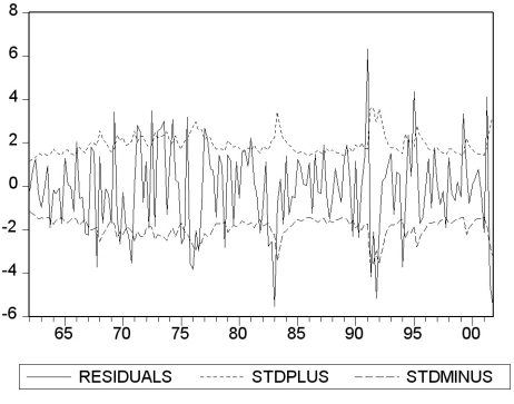 Describe what you see.
t = 1.17 - .56 ΔInft-1 - .47 ΔInft-2 - .31 ΔInft-3 - .13 Unempt-1(.48)(.08)(.10)(.09)(.06)
= .86 + .27 + .53 .(.40)(.11)(.15)
(a)Test the two coefficients for
and in the GARCH model individually for statistical significance.(b)Estimating the same equation by OLS results in
t = 1.19 - .51 ΔInft-1 - .47 ΔInft-2 - .28 ΔInft-3 - .16Unempt-1(.54)(.10)(.11)(.08)(.07)
Briefly compare the estimates.Which of the two methods do you prefer?
(c)Given your results from the test in (a),what can you say about the variance of the error terms in the Phillips Curve for Canada?
(d)The following figure plots the residuals along with bands of plus or minus one predicted standard deviation (that is,±
)based on the GARCH(1,1)model. Describe what you see. سؤال
سؤال
Consider the GARCH(1,1)model  = α0 + α1
  + φ1
+ φ1  .Show that this model can be rewritten as
  =
=  + α1(
+ α1(  + φ1
+ φ1  +
+ 
 +
+ 
 + ... ).(Hint: use the GARCH(1,1)model but specify it for
  ;substitute this expression into the original specification,and so on. )Explain intuitively the meaning of the resulting formulation.
= α0 + α1 + φ1 .Show that this model can be rewritten as = + α1( + φ1 + + + ... ).(Hint: use the GARCH(1,1)model but specify it for ;substitute this expression into the original specification,and so on. )Explain intuitively the meaning of the resulting formulation. سؤال
سؤال
سؤال
سؤال
سؤال
سؤال
سؤال
There has been much talk recently about the convergence of inflation rates between many of the OECD economies.You want to see if there is evidence of this closer to home by checking whether or not Canada's inflation rate and the United States' inflation rate are cointegrated.
(a)You begin your numerical analysis by testing for a stochastic trend in the variables,using an Augmented Dickey-Fuller test.The t-statistic for the coefficient of interest is as follows:
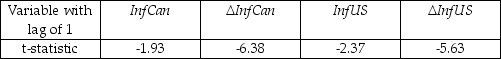 where InfCan is the Canadian inflation rate,and InfUS is the United States inflation rate.The estimated equation included an intercept.For each case make a decision about the stationarity of the variables based on the critical value of the Augmented Dickey-Fuller test statistic.
(b)Your test for cointegration results in a EG-ADF statistic of (-7.34).Can you reject the null hypothesis of a unit root for the residuals from the cointegrating regression?
(c)Using a working hypothesis that the two inflation rates are cointegrated,you want to test whether or not the slope coefficient equals one.To do so you estimate the cointegrating equation using the DOLS estimator with HAC standard errors.The coefficient on the U.S.inflation rate has a value of 0.45 with a standard error of 0.13.Can you reject the null hypothesis that the slope equals unity?
(d)Even if you could not reject the null hypothesis of a unit slope,would that have been sufficient evidence to establish convergence?
(a)You begin your numerical analysis by testing for a stochastic trend in the variables,using an Augmented Dickey-Fuller test.The t-statistic for the coefficient of interest is as follows:
where InfCan is the Canadian inflation rate,and InfUS is the United States inflation rate.The estimated equation included an intercept.For each case make a decision about the stationarity of the variables based on the critical value of the Augmented Dickey-Fuller test statistic.(b)Your test for cointegration results in a EG-ADF statistic of (-7.34).Can you reject the null hypothesis of a unit root for the residuals from the cointegrating regression?
(c)Using a working hypothesis that the two inflation rates are cointegrated,you want to test whether or not the slope coefficient equals one.To do so you estimate the cointegrating equation using the DOLS estimator with HAC standard errors.The coefficient on the U.S.inflation rate has a value of 0.45 with a standard error of 0.13.Can you reject the null hypothesis that the slope equals unity?
(d)Even if you could not reject the null hypothesis of a unit slope,would that have been sufficient evidence to establish convergence?
سؤال
In this case,the Granger causality statistic does not exceed the critical value,and hence the conclusion is that the change in the inflation rate does not Granger-cause the unemployment rate.  t = 0.05 - 0.31 ΔInft-1
(0.14)(0.07)
t = 1982:I - 2009:IV,R2 = 0.10,SER = 2.4
a.Calculate the one-quarter-ahead forecast of both ΔInf2010:I and Inf2010:I (the inflation rate in 2009:IV was 2.6 percent,and the change in the inflation rate for that quarter was -1.04).
b.Calculate the forecast for 2010:II using the iterated multiperiod AR forecast both for the change in the inflation rate and the inflation rate.
c.What alternative method could you have used to forecast two quarters ahead? Write down the equation for the two-period ahead forecast,using parameters instead of numerical coefficients,which you would have used.
t = 0.05 - 0.31 ΔInft-1(0.14)(0.07)
t = 1982:I - 2009:IV,R2 = 0.10,SER = 2.4
a.Calculate the one-quarter-ahead forecast of both ΔInf2010:I and Inf2010:I (the inflation rate in 2009:IV was 2.6 percent,and the change in the inflation rate for that quarter was -1.04).
b.Calculate the forecast for 2010:II using the iterated multiperiod AR forecast both for the change in the inflation rate and the inflation rate.
c.What alternative method could you have used to forecast two quarters ahead? Write down the equation for the two-period ahead forecast,using parameters instead of numerical coefficients,which you would have used.
سؤال
سؤال
Your textbook states that there "are three ways to decide if two variables can plausibly be modeled as cointegrated: use expert knowledge and economic theory,graph the series and see whether they appear to have a common stochastic trend,and perform statistical tests for cointegration.All three ways should be used in practice." Accordingly you set out to check whether (the log of)consumption and (the log of)personal disposable income are cointegrated.You collect data for the sample period 1962:I to 1995:IV and plot the two variables. 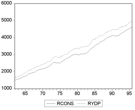 (a)Using the first two methods to examine the series for cointegration,what do you think the likely answer is?
(b)You begin your numerical analysis by testing for a stochastic trend in the variables,using an Augmented Dickey-Fuller test.The t-statistic for the coefficient of interest is as follows:
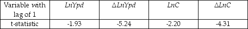 where LnYpd is (the log of)personal disposable income,and LnC is (the log of)real consumption.The estimated equation included an intercept for the two growth rates,and,in addition,a deterministic trend for the level variables.For each case make a decision about the stationarity of the variables based on the critical value of the Augmented Dickey-Fuller test statistic.Why do you think a trend was included for level variables?
(c)Using the first step of the EG-ADF procedure,you get the following result: t = -0.24 + 1.017 lnYpdt
Should you interpret this equation? Would you be impressed if you were told that the regression R2 was 0.998 and that the t-statistic for the slope was 266.06? Why or why not?
(d)The Dickey-Fuller test for the residuals for the cointegrating regressions results in a t-statistic of
(-3.64).State the null and alternative hypothesis and make a decision based on the result.
(e)You want to investigate if the slope of the cointegrating vector is one.To do so,you use the DOLS estimator and HAC standard errors.The slope coefficient is 1.024 with a standard error of 0.009.Can you reject the null hypothesis that the slope equals one?
(a)Using the first two methods to examine the series for cointegration,what do you think the likely answer is?(b)You begin your numerical analysis by testing for a stochastic trend in the variables,using an Augmented Dickey-Fuller test.The t-statistic for the coefficient of interest is as follows:
where LnYpd is (the log of)personal disposable income,and LnC is (the log of)real consumption.The estimated equation included an intercept for the two growth rates,and,in addition,a deterministic trend for the level variables.For each case make a decision about the stationarity of the variables based on the critical value of the Augmented Dickey-Fuller test statistic.Why do you think a trend was included for level variables?(c)Using the first step of the EG-ADF procedure,you get the following result:
t = -0.24 + 1.017 lnYpdtShould you interpret this equation? Would you be impressed if you were told that the regression R2 was 0.998 and that the t-statistic for the slope was 266.06? Why or why not?
(d)The Dickey-Fuller test for the residuals for the cointegrating regressions results in a t-statistic of
(-3.64).State the null and alternative hypothesis and make a decision based on the result.
(e)You want to investigate if the slope of the cointegrating vector is one.To do so,you use the DOLS estimator and HAC standard errors.The slope coefficient is 1.024 with a standard error of 0.009.Can you reject the null hypothesis that the slope equals one?
سؤال
You have collected quarterly data for real GDP (Y)for the United States for the period 1962:I (first quarter)to 2009:IV.
a.Testing the log of GDP for stationarity,you run the following regression (where the lag length was determined using the AIC): t = 0.03 - 0.0024 lnYt-1 + 0.253 ΔlnYt-1 + 0.167 ΔlnYt-2
(0.03)(0.0014)(0.072)(0.072)
t = 1962:I - 2009:IV,R2 = 0.16,SER = 0.008
Use the ADF statistic with an intercept only to test for stationarity.What is your decision?
b.You have decided to test the growth rate of real GDP for stationarity for the same sample period.The regression is as follows: t = 0.0041 - 0.543 ΔlnYt-1 - 0.186 Δ2lnYt-1
(0.0009)(0.082)(0.071)
t = 1962:I - 2009:IV,R2 = 0.16,SER = 0.008
Use the ADF statistic with an intercept only to test for stationarity.What is your decision?
c.Using the orders of integration terminology,what order of integration is the log level of real GDP? The growth rate?
d.Given that the SER hardly changed in the second equation,why is the regression R2 larger?
a.Testing the log of GDP for stationarity,you run the following regression (where the lag length was determined using the AIC):
t = 0.03 - 0.0024 lnYt-1 + 0.253 ΔlnYt-1 + 0.167 ΔlnYt-2(0.03)(0.0014)(0.072)(0.072)
t = 1962:I - 2009:IV,R2 = 0.16,SER = 0.008
Use the ADF statistic with an intercept only to test for stationarity.What is your decision?
b.You have decided to test the growth rate of real GDP for stationarity for the same sample period.The regression is as follows:
t = 0.0041 - 0.543 ΔlnYt-1 - 0.186 Δ2lnYt-1(0.0009)(0.082)(0.071)
t = 1962:I - 2009:IV,R2 = 0.16,SER = 0.008
Use the ADF statistic with an intercept only to test for stationarity.What is your decision?
c.Using the orders of integration terminology,what order of integration is the log level of real GDP? The growth rate?
d.Given that the SER hardly changed in the second equation,why is the regression R2 larger?
سؤال
Consider the following model Yt = β0 + β1Xt + β2Xt-1 + β3Yt-1 + ut,where Xt is strictly exogenous.Show that by imposing the restriction  ,you can derive the following so-called Error Correction Mechanism (ECM)model
△Yt = β0 + β1△Xt - θ(Y - X)t-1 + ut
where θ = β1 + β2.What is the short-run (impact)response of a unit increase in X? What is the long-run solution? Why do you think the term in parenthesis in the above expression is called ECM?
,you can derive the following so-called Error Correction Mechanism (ECM)model△Yt = β0 + β1△Xt - θ(Y - X)t-1 + ut
where θ = β1 + β2.What is the short-run (impact)response of a unit increase in X? What is the long-run solution? Why do you think the term in parenthesis in the above expression is called ECM?
سؤال
Economic theory suggests that the law of one price holds.Applying this concept to foreign and domestic goods implies that goods will sell for the same price across countries.The consumer price index is the price for a basket of goods,and is calculated for countries as a whole.Hence in the absence of barriers to trade,and large transportation costs (and the fact that not all goods are traded)you should observe Purchasing Power Parity (PPP)between two countries,or ExchRate × P = Pf,where ExchRate is the foreign exchange rate between the two countries,and P represents the price index,with f indicating the foreign country.Dividing both sides of the equation by the domestic price level then gives you the standard formulation for PPP: ExchRate =  .If PPP holds in the long run,then the exchange rate and the price ratio should share a common trend.Since it is a long-run concept,cointegration provides an interesting way to test for it.
a.Using monthly data for the U.S./U.K.exchange rate ($/₤)and the respective price indexes,you estimate the following regression: t = 0.44 + 0.69 (lnPUS - lnPUK)
Collecting the residuals from this regression and using an ADF test for cointegration,you find a t-statistic of -2.71.Can you reject the null-hypothesis of no cointegration? What is the critical value?
b.Was it good econometric practice to test for cointegration right away? What else should you have done before proceeding with the EG-ADF test?
.If PPP holds in the long run,then the exchange rate and the price ratio should share a common trend.Since it is a long-run concept,cointegration provides an interesting way to test for it.a.Using monthly data for the U.S./U.K.exchange rate ($/₤)and the respective price indexes,you estimate the following regression:
t = 0.44 + 0.69 (lnPUS - lnPUK)Collecting the residuals from this regression and using an ADF test for cointegration,you find a t-statistic of -2.71.Can you reject the null-hypothesis of no cointegration? What is the critical value?
b.Was it good econometric practice to test for cointegration right away? What else should you have done before proceeding with the EG-ADF test?
سؤال
سؤال

فتح الحزمة
قم بالتسجيل لفتح البطاقات في هذه المجموعة!
Unlock Deck
Unlock Deck
1/50
العب
ملء الشاشة (f)
Deck 16: Additional Topics in Time Series Regression
1
Multiperiod forecasting with multiple predictors
A)is the same as the iterated AR forecast method.
B)can use the iterated VAR forecast method.
C)will yield superior results when using the multiperiod regression forecast h periods into the future based on p lags of each Yt ,rather than the iterated VAR forecast method.
D)will always yield superior results using the iterated VAR since it takes all equations into account.
B
2
Unit root tests
A)use the standard normal distribution since they are based on the t-statistic.
B)cannot use the standard normal distribution for statistical inference.As a result the ADF statistic has its own special table of critical values.
C)can use the standard normal distribution only when testing that the level variable is stationary,but not the difference variable.
D)can use the standard normal distribution but only if HAC standard errors were computed.
B
3
A VAR with five variables,4 lags and constant terms for each equation will have a total of
A)21 coefficients.
B)100 coefficients.
C)105 coefficients.
D)84 coefficients.
A)21 coefficients.
B)100 coefficients.
C)105 coefficients.
D)84 coefficients.
C
4
The error term in a multiperiod regression
A)is serially correlated.
B)causes OLS to be inconsistent.
C)is serially correlated,but less so the longer the forecast horizon.
D)is serially uncorrelated.
A)is serially correlated.
B)causes OLS to be inconsistent.
C)is serially correlated,but less so the longer the forecast horizon.
D)is serially uncorrelated.
فتح الحزمة
افتح القفل للوصول البطاقات البالغ عددها 50 في هذه المجموعة.
فتح الحزمة
k this deck
5
One advantage of forecasts based on a VAR rather than separately forecasting the variables involved is
A)that VAR forecasts are easier to calculate.
B)you typically have knowledge of future values of at least one of the variables involved.
C)it can help to make the forecasts mutually consistent.
D)that VAR involves panel data.
A)that VAR forecasts are easier to calculate.
B)you typically have knowledge of future values of at least one of the variables involved.
C)it can help to make the forecasts mutually consistent.
D)that VAR involves panel data.
فتح الحزمة
افتح القفل للوصول البطاقات البالغ عددها 50 في هذه المجموعة.
فتح الحزمة
k this deck
6
A vector autoregression
A)is the ADL model with an AR process in the error term.
B)is the same as a univariate autoregression.
C)is a set of k time series regressions,in which the regressors are lagged values of all k series.
D)involves errors that are autocorrelated but can be written in vector format.
A)is the ADL model with an AR process in the error term.
B)is the same as a univariate autoregression.
C)is a set of k time series regressions,in which the regressors are lagged values of all k series.
D)involves errors that are autocorrelated but can be written in vector format.
فتح الحزمة
افتح القفل للوصول البطاقات البالغ عددها 50 في هذه المجموعة.
فتح الحزمة
k this deck
7
The order of integration
A)can never be zero.
B)is the number of times that the series needs to be differenced for it to be stationary.
C)is the value of φ1 in the quasi difference(ΔYt - φ1Yt-1).
D)depends on the number of lags in the VAR specification.
A)can never be zero.
B)is the number of times that the series needs to be differenced for it to be stationary.
C)is the value of φ1 in the quasi difference(ΔYt - φ1Yt-1).
D)depends on the number of lags in the VAR specification.
فتح الحزمة
افتح القفل للوصول البطاقات البالغ عددها 50 في هذه المجموعة.
فتح الحزمة
k this deck
8
In a VECM,
A)past values of Yt - θ Xt help to predict future values of ΔYt and/or ΔXt.
B)errors are corrected for serial correlation using the Cochrane-Orcutt method.
C)current values of Yt - θ Xt help to predict future values of ΔYt and/or ΔXt.
D)VAR techniques,such as information criteria,no longer apply.
A)past values of Yt - θ Xt help to predict future values of ΔYt and/or ΔXt.
B)errors are corrected for serial correlation using the Cochrane-Orcutt method.
C)current values of Yt - θ Xt help to predict future values of ΔYt and/or ΔXt.
D)VAR techniques,such as information criteria,no longer apply.
فتح الحزمة
افتح القفل للوصول البطاقات البالغ عددها 50 في هذه المجموعة.
فتح الحزمة
k this deck
9
If Yt is I(2),then
A)Δ2Yt is stationary.
B)Yt has a unit autoregressive root.
C)ΔYt is stationary.
D)Yt is stationary.
A)Δ2Yt is stationary.
B)Yt has a unit autoregressive root.
C)ΔYt is stationary.
D)Yt is stationary.
فتح الحزمة
افتح القفل للوصول البطاقات البالغ عددها 50 في هذه المجموعة.
فتح الحزمة
k this deck
10
If Xt and Yt are cointegrated,then the OLS estimator of the coefficient in the cointegrating regression is
A)BLUE.
B)unbiased when using HAC standard errors.
C)unbiased even in small samples.
D)consistent.
A)BLUE.
B)unbiased when using HAC standard errors.
C)unbiased even in small samples.
D)consistent.
فتح الحزمة
افتح القفل للوصول البطاقات البالغ عددها 50 في هذه المجموعة.
فتح الحزمة
k this deck
11
To test the null hypothesis of a unit root,the ADF test
A)has higher power than the so-called DF-GLS test.
B)uses complicated interative techniques.
C)cannot be calculated if the variable is integrated of order two or higher.
D)uses a t-statistic and a special critical value.
A)has higher power than the so-called DF-GLS test.
B)uses complicated interative techniques.
C)cannot be calculated if the variable is integrated of order two or higher.
D)uses a t-statistic and a special critical value.
فتح الحزمة
افتح القفل للوصول البطاقات البالغ عددها 50 في هذه المجموعة.
فتح الحزمة
k this deck
12
The following is not a consequence of Xt and Yt being cointegrated:
A)if Xt and Yt are both I(1),then for some θ,Yt - θ Xt is I(0).
B)Xt and Yt have the same stochastic trend.
C)in the expression Yt - θ Xt ,θ is called the cointegrating coefficient.
D)if Xt and Yt are cointegrated then integrating one of the variables gives you the same result as integrating the other.
فتح الحزمة
افتح القفل للوصول البطاقات البالغ عددها 50 في هذه المجموعة.
فتح الحزمة
k this deck
13
The following is not an appropriate way to tell whether two variables are cointegrated:
A)see if the two variables are integrated of the same order.
B)graph the series and see whether they appear to have a common stochastic trend.
C)perform statistical tests for cointegration.
D)use expert knowledge and economic theory.
A)see if the two variables are integrated of the same order.
B)graph the series and see whether they appear to have a common stochastic trend.
C)perform statistical tests for cointegration.
D)use expert knowledge and economic theory.
فتح الحزمة
افتح القفل للوصول البطاقات البالغ عددها 50 في هذه المجموعة.
فتح الحزمة
k this deck
14
The coefficients of the VAR are estimated by
A)using a simultaneous estimation method such as TSLS.
B)maximum likelihood.
C)panel methods.
D)estimating each of the equations by OLS.
A)using a simultaneous estimation method such as TSLS.
B)maximum likelihood.
C)panel methods.
D)estimating each of the equations by OLS.
فتح الحزمة
افتح القفل للوصول البطاقات البالغ عددها 50 في هذه المجموعة.
فتح الحزمة
k this deck
15
Δ2Yt
A)= ΔYt - ΔYt-1.
B)= -
.
C)= ΔYt -ΔYt-2.
D)= Yt - Yt-2.
A)= ΔYt - ΔYt-1.
B)=
- .C)= ΔYt -ΔYt-2.
D)= Yt - Yt-2.
فتح الحزمة
افتح القفل للوصول البطاقات البالغ عددها 50 في هذه المجموعة.
فتح الحزمة
k this deck
16
The biggest conceptual difference between using VARs for forecasting and using them for structural modeling is that
A)you need to use the Granger causality test for structural modeling.
B)structural modeling requires very specific assumptions derived from economic theory and institutional knowledge of what is exogenous and what is not.
C)you can no longer use the information criteria to decide on the lag length.
D)structural modeling only allows a maximum of three equations in the VAR.
فتح الحزمة
افتح القفل للوصول البطاقات البالغ عددها 50 في هذه المجموعة.
فتح الحزمة
k this deck
17
A multiperiod regression forecast h periods into the future based on an AR(p)is computed
A)the same way as the iterated AR forecast.
B)by estimating the multiperiod regression Yt = δ0 + δ1Yt-h + ...+ δpYt-p-h+1 + ut,then using the estimated coefficients to compute the forecast h periods in advance.
C)by estimating the multiperiod regression Yt = δ0 + δ1Yt-h + ut ,then using the estimate coefficients to compute the forecast h period in advance.
D)by first computing the one-period ahead forecast,next using that to compute the two-period ahead forecast,and so forth.
فتح الحزمة
افتح القفل للوصول البطاقات البالغ عددها 50 في هذه المجموعة.
فتح الحزمة
k this deck
18
You can determine the lag lengths in a VAR
A)by using confidence intervals.
B)by using critical values from the standard normal table.
C)by using either F-tests or information criteria.
D)with the help from economic theory and institutional knowledge.
A)by using confidence intervals.
B)by using critical values from the standard normal table.
C)by using either F-tests or information criteria.
D)with the help from economic theory and institutional knowledge.
فتح الحزمة
افتح القفل للوصول البطاقات البالغ عددها 50 في هذه المجموعة.
فتح الحزمة
k this deck
19
Under the VAR assumptions,the OLS estimators are
A)consistent and have a joint normal distribution even in small samples.
B)BLUE.
C)consistent and have a joint normal distribution in large samples.
D)unbiased.
A)consistent and have a joint normal distribution even in small samples.
B)BLUE.
C)consistent and have a joint normal distribution in large samples.
D)unbiased.
فتح الحزمة
افتح القفل للوصول البطاقات البالغ عددها 50 في هذه المجموعة.
فتح الحزمة
k this deck
20
A VAR allows you to test joint hypothesis that involve restrictions across multiple equations by
A)computing a z-statistic.
B)computing the BIC but not the AIC.
C)using a stability test.
D)computing an F-statistic.
A)computing a z-statistic.
B)computing the BIC but not the AIC.
C)using a stability test.
D)computing an F-statistic.
فتح الحزمة
افتح القفل للوصول البطاقات البالغ عددها 50 في هذه المجموعة.
فتح الحزمة
k this deck
21
You have collected quarterly data on inflation and unemployment rates for Canada from 1961:III to 1995:IV to estimate a VAR(4)model of the change in the rate of inflation and the unemployment rate.The results are t = 1.02 - .54 ΔInft-1 - .46 ΔInft-2 - .32 ΔInft-2 - .01 ΔInft-4
.09)(.09)(.09)(.08)(.44)
-.76 Unempt-1 + .20 Unempt-2 - .16 Unempt-3 + .59 Unempt-4
(.43)(.76)(.76)(.44) = .26. t = 0.18 - .003 ΔInft-1 - .016 ΔInft-2 - .018 ΔInft-3 - .010 ΔInft-4
(.10)(.016)(.018)(.017)(.016)
+ 1.47 Unempt-1 - .46 Unempt-2 - .08 Unempt-3 + .05 Unempt-4
(.08)(.14)(.14)(.08) = .980.
(a)Explain how you would use the above regressions to conduct one period ahead forecasts.
(b)Should you test for cointegration between the change in the inflation rate and the unemployment rate and,in the case of finding cointegration here,respecify the above model as a VECM?
(c)The Granger causality test yields the following F-statistics: 3.75 for the test that the coefficients on lagged unemployment rate in the change of inflation equation are all zero;and 0.36 for the test that the coefficients on lagged changes in the inflation rate are all zero.Based on these results,does unemployment Granger-cause inflation? Does inflation Granger-cause unemployment?
t = 1.02 - .54 ΔInft-1 - .46 ΔInft-2 - .32 ΔInft-2 - .01 ΔInft-4.09)(.09)(.09)(.08)(.44)
-.76 Unempt-1 + .20 Unempt-2 - .16 Unempt-3 + .59 Unempt-4
(.43)(.76)(.76)(.44)
= .26. t = 0.18 - .003 ΔInft-1 - .016 ΔInft-2 - .018 ΔInft-3 - .010 ΔInft-4(.10)(.016)(.018)(.017)(.016)
+ 1.47 Unempt-1 - .46 Unempt-2 - .08 Unempt-3 + .05 Unempt-4
(.08)(.14)(.14)(.08)
= .980.(a)Explain how you would use the above regressions to conduct one period ahead forecasts.
(b)Should you test for cointegration between the change in the inflation rate and the unemployment rate and,in the case of finding cointegration here,respecify the above model as a VECM?
(c)The Granger causality test yields the following F-statistics: 3.75 for the test that the coefficients on lagged unemployment rate in the change of inflation equation are all zero;and 0.36 for the test that the coefficients on lagged changes in the inflation rate are all zero.Based on these results,does unemployment Granger-cause inflation? Does inflation Granger-cause unemployment?
فتح الحزمة
افتح القفل للوصول البطاقات البالغ عددها 50 في هذه المجموعة.
فتح الحزمة
k this deck
22
You have collected quarterly data for the unemployment rate (Unemp)in the United States,using a sample period from 1962:I (first quarter)to 2009:IV (the data is collected at a monthly frequency,but you have taken quarterly averages).
a.Does economic theory suggest that the unemployment rate should be stationary?
b.Testing the unemployment rate for stationarity,you run the following regression (where the lag length was determined using the BIC;using the AIC instead does not change the outcome of the test,even though it chooses 9 lags of the LHS variable): t = 0.217 - 0.035 Unempt-1 + 0.689 ΔUnempt-1
(0.01)0.0012)(0.054)
Use the ADF statistic with an intercept only to test for stationarity.What is your decision?
c.The standard errors reported above were homoskedasticity-only standard errors.Do you think you could potentially improve on inference by allowing for HAC standard errors?
d.An alternative test for a unit root,the DF-GLS,produces a test statistic of -2.75.Find the critical value and decide whether or not to reject the null hypothesis.If the decision is different from (c),is there any reason why you might prefer the DF-GLS test over the ADF test?
a.Does economic theory suggest that the unemployment rate should be stationary?
b.Testing the unemployment rate for stationarity,you run the following regression (where the lag length was determined using the BIC;using the AIC instead does not change the outcome of the test,even though it chooses 9 lags of the LHS variable):
t = 0.217 - 0.035 Unempt-1 + 0.689 ΔUnempt-1(0.01)0.0012)(0.054)
Use the ADF statistic with an intercept only to test for stationarity.What is your decision?
c.The standard errors reported above were homoskedasticity-only standard errors.Do you think you could potentially improve on inference by allowing for HAC standard errors?
d.An alternative test for a unit root,the DF-GLS,produces a test statistic of -2.75.Find the critical value and decide whether or not to reject the null hypothesis.If the decision is different from (c),is there any reason why you might prefer the DF-GLS test over the ADF test?
فتح الحزمة
افتح القفل للوصول البطاقات البالغ عددها 50 في هذه المجموعة.
فتح الحزمة
k this deck
23
The lag length in a VAR using the BIC proceeds as follows: Among a set of candidate values of p,the estimated lag length xxxis the value of p
A)For which the BIC exceeds the AIC
B)That maximizes BIC(p)
C)Cannot be determined here since a VAR is a system of equations,not a single one
D)That minimizes BIC(p)
A)For which the BIC exceeds the AIC
B)That maximizes BIC(p)
C)Cannot be determined here since a VAR is a system of equations,not a single one
D)That minimizes BIC(p)
فتح الحزمة
افتح القفل للوصول البطاقات البالغ عددها 50 في هذه المجموعة.
فتح الحزمة
k this deck
24
What role does the concept of cointegration and the order of integration play in modeling the relationship between variables? Explain how tests of cointegration work.
فتح الحزمة
افتح القفل للوصول البطاقات البالغ عددها 50 في هذه المجموعة.
فتح الحزمة
k this deck
25
The DOLS estimator has the following property if Xt and Yt are cointegrated:
A)it is BLUE even in small samples.
B)it is efficient in large samples.
C)it has a standard normal distribution when homoskedasticity-only standard errors are used.
D)it has a non-normal distribution in large samples when HAC standard errors are used.
A)it is BLUE even in small samples.
B)it is efficient in large samples.
C)it has a standard normal distribution when homoskedasticity-only standard errors are used.
D)it has a non-normal distribution in large samples when HAC standard errors are used.
فتح الحزمة
افتح القفل للوصول البطاقات البالغ عددها 50 في هذه المجموعة.
فتح الحزمة
k this deck
26
Using the ADL(1,1)regression Yt = β0 + β1Yt-1 + Xt-1 + ut,the ARCH model for the regression error assumes that ut is normally distributed with mean zero and variance ,where
A) = α0 + α1
+ α2
+ ...+ αp
.
B) =
+ ...+
+ φ1
+ ...+ φq
.
C) = φ1
+ ...+ φq
.
D) = α0 + α1
+ ...+ αp
+ φ1
+ ...+ φq
.
Xt-1 + ut,the ARCH model for the regression error assumes that ut is normally distributed with mean zero and variance ,whereA)
= α0 + α1 + α2 + ...+ αp .B)
= + ...+ + φ1 + ...+ φq .C)
= φ1 + ...+ φq .D)
= α0 + α1 + ...+ αp + φ1 + ...+ φq . فتح الحزمة
افتح القفل للوصول البطاقات البالغ عددها 50 في هذه المجموعة.
فتح الحزمة
k this deck
27
The dynamic OLS (DOLS)estimator of the cointegrating coefficient,if Yt and Xt are cointegrated,
A)is efficient in large samples
B)statistical inference about the cointegrating coefficient is valid
C)the t-statistic constructed using the DOLS estimator with HAC standard errors has a standard normal distribution in large samples
D)all of the above
A)is efficient in large samples
B)statistical inference about the cointegrating coefficient is valid
C)the t-statistic constructed using the DOLS estimator with HAC standard errors has a standard normal distribution in large samples
D)all of the above
فتح الحزمة
افتح القفل للوصول البطاقات البالغ عددها 50 في هذه المجموعة.
فتح الحزمة
k this deck
28
The BIC for the VAR is
A)BIC(p)= ln[det ( u)] + k(kp+1)
B)BIC(p)= ln[det ( u)] + k(p+1)
C)BIC(p)= ln[det ( u)] + k(kp+1)
D)BIC(p)= ln[SSR(p)] + k(p+1)
A)BIC(p)= ln[det (
u)] + k(kp+1)B)BIC(p)= ln[det (
u)] + k(p+1)C)BIC(p)= ln[det (
u)] + k(kp+1)D)BIC(p)= ln[SSR(p)] + k(p+1)
فتح الحزمة
افتح القفل للوصول البطاقات البالغ عددها 50 في هذه المجموعة.
فتح الحزمة
k this deck
29
Volatility clustering
A)is evident in most cross-sections.
B)implies that a series is serially correlated.
C)can mostly be found in studies of the labor market.
D)is evident in many financial time series.
A)is evident in most cross-sections.
B)implies that a series is serially correlated.
C)can mostly be found in studies of the labor market.
D)is evident in many financial time series.
فتح الحزمة
افتح القفل للوصول البطاقات البالغ عددها 50 في هذه المجموعة.
فتح الحزمة
k this deck
30
A VAR with k time series variables consists of
A)k equations,one for each of the variables,where the regressors in all equations are lagged values of all the variables
B)a single equation,where the regressors are lagged values of all the variables
C)k equations,one for each of the variables,where the regressors in all equations are never more than one lag of all the variables
D)k equations,one for each of the variables,where the regressors in all equations are current values of all the variables
فتح الحزمة
افتح القفل للوصول البطاقات البالغ عددها 50 في هذه المجموعة.
فتح الحزمة
k this deck
31
Purchasing power parity (PPP),postulates that the exchange rate between two countries equals the ratio of the respective price indexes or ExchRate = (where ExchRate is the foreign exchange rate between the two countries,and P represents the price index,with f indicating the foreign country).The long-run version of PPP implies that that the exchange rate and the price ratio share a common trend.
(a)You collect monthly foreign exchange rate data from 1974:1 to 2002:4 for the U.S./U.K.exchange rate ($/£)and you collect data on the Consumer Price Index for both countries.Explain how you would used the Engle-Granger test statistic to investigate the long-run PPP hypothesis.
(b)One of your peers explains that there may be an easier way to test for the validity of PPP.She suggests to simply test whether or not the "real" exchange rate,or competitiveness,is stationary.(The real exchange rate is given by ExchRate × )Is she correct? Explain.How would you implement her suggestion? Which alternative test-statistic is available?
(where ExchRate is the foreign exchange rate between the two countries,and P represents the price index,with f indicating the foreign country).The long-run version of PPP implies that that the exchange rate and the price ratio share a common trend.(a)You collect monthly foreign exchange rate data from 1974:1 to 2002:4 for the U.S./U.K.exchange rate ($/£)and you collect data on the Consumer Price Index for both countries.Explain how you would used the Engle-Granger test statistic to investigate the long-run PPP hypothesis.
(b)One of your peers explains that there may be an easier way to test for the validity of PPP.She suggests to simply test whether or not the "real" exchange rate,or competitiveness,is stationary.(The real exchange rate is given by ExchRate ×
)Is she correct? Explain.How would you implement her suggestion? Which alternative test-statistic is available? فتح الحزمة
افتح القفل للوصول البطاقات البالغ عددها 50 في هذه المجموعة.
فتح الحزمة
k this deck
32
Think of at least five examples from economics where theory suggests that the variables involved are cointegrated.For one of these cases,explain how you would test for cointegration between the variables involved and how you could use this information to improve forecasting.
فتح الحزمة
افتح القفل للوصول البطاقات البالغ عددها 50 في هذه المجموعة.
فتح الحزمة
k this deck
33
You have collected quarterly Canadian data on the unemployment and the inflation rate from 1962:I to 2001:IV.You want to re-estimate the ADL(3,1)formulation of the Phillips curve using a GARCH(1,1)specification.The results are as follows: t = 1.17 - .56 ΔInft-1 - .47 ΔInft-2 - .31 ΔInft-3 - .13 Unempt-1
(.48)(.08)(.10)(.09)(.06) = .86 + .27 + .53 .
(.40)(.11)(.15)
(a)Test the two coefficients for and in the GARCH model individually for statistical significance.
(b)Estimating the same equation by OLS results in t = 1.19 - .51 ΔInft-1 - .47 ΔInft-2 - .28 ΔInft-3 - .16Unempt-1
(.54)(.10)(.11)(.08)(.07)
Briefly compare the estimates.Which of the two methods do you prefer?
(c)Given your results from the test in (a),what can you say about the variance of the error terms in the Phillips Curve for Canada?
(d)The following figure plots the residuals along with bands of plus or minus one predicted standard deviation (that is,± )based on the GARCH(1,1)model. Describe what you see.
t = 1.17 - .56 ΔInft-1 - .47 ΔInft-2 - .31 ΔInft-3 - .13 Unempt-1(.48)(.08)(.10)(.09)(.06)
= .86 + .27 + .53 .(.40)(.11)(.15)
(a)Test the two coefficients for
and in the GARCH model individually for statistical significance.(b)Estimating the same equation by OLS results in
t = 1.19 - .51 ΔInft-1 - .47 ΔInft-2 - .28 ΔInft-3 - .16Unempt-1(.54)(.10)(.11)(.08)(.07)
Briefly compare the estimates.Which of the two methods do you prefer?
(c)Given your results from the test in (a),what can you say about the variance of the error terms in the Phillips Curve for Canada?
(d)The following figure plots the residuals along with bands of plus or minus one predicted standard deviation (that is,±
)based on the GARCH(1,1)model. Describe what you see. فتح الحزمة
افتح القفل للوصول البطاقات البالغ عددها 50 في هذه المجموعة.
فتح الحزمة
k this deck
34
Carefully explain the difference between forecasting variables separately versus forecasting a vector of time series variables.Mention how you choose optimal lag lengths in each case.Part of your essay should deal with multiperiod forecasts and different methods that can be used in that situation.Finally address the difference between VARS and VECM.
فتح الحزمة
افتح القفل للوصول البطاقات البالغ عددها 50 في هذه المجموعة.
فتح الحزمة
k this deck
35
Consider the GARCH(1,1)model = α0 + α1 + φ1 .Show that this model can be rewritten as = + α1( + φ1 + + + ... ).(Hint: use the GARCH(1,1)model but specify it for ;substitute this expression into the original specification,and so on. )Explain intuitively the meaning of the resulting formulation.
= α0 + α1 + φ1 .Show that this model can be rewritten as = + α1( + φ1 + + + ... ).(Hint: use the GARCH(1,1)model but specify it for ;substitute this expression into the original specification,and so on. )Explain intuitively the meaning of the resulting formulation. فتح الحزمة
افتح القفل للوصول البطاقات البالغ عددها 50 في هذه المجموعة.
فتح الحزمة
k this deck
36
Assume that you have used the OLS estimator in the cointegrating regression and test the residual for a unit root using an ADF test.The resulting ADF test statistic has a
A)normal distribution in large samples.
B)non-normal distribution which requires ADF critical values for inference.
C)non-normal distribution which requires EG-ADF critical values for inference.
D)normal distribution when HAC standard errors are used.
A)normal distribution in large samples.
B)non-normal distribution which requires ADF critical values for inference.
C)non-normal distribution which requires EG-ADF critical values for inference.
D)normal distribution when HAC standard errors are used.
فتح الحزمة
افتح القفل للوصول البطاقات البالغ عددها 50 في هذه المجموعة.
فتح الحزمة
k this deck
37
ARCH and GARCH models are estimated using the
A)OLS estimation method.
B)the method of maximum likelihood.
C)DOLS estimation method.
D)VAR specification.
A)OLS estimation method.
B)the method of maximum likelihood.
C)DOLS estimation method.
D)VAR specification.
فتح الحزمة
افتح القفل للوصول البطاقات البالغ عددها 50 في هذه المجموعة.
فتح الحزمة
k this deck
38
Some macroeconomic theories suggest that there is a short-run relationship between the inflation rate and the unemployment rate.How would you go about forecasting these two variables? Suggest various alternatives and discuss their advantages and disadvantages.
فتح الحزمة
افتح القفل للوصول البطاقات البالغ عددها 50 في هذه المجموعة.
فتح الحزمة
k this deck
39
The EG-ADF test
A)is the similar to the DF-GLS test
B)is a test for cointegration
C)has as a limitation that it can only test if two variables,but not more than two,are cointegrated
D)uses the ADF in the second step of its procedure
A)is the similar to the DF-GLS test
B)is a test for cointegration
C)has as a limitation that it can only test if two variables,but not more than two,are cointegrated
D)uses the ADF in the second step of its procedure
فتح الحزمة
افتح القفل للوصول البطاقات البالغ عددها 50 في هذه المجموعة.
فتح الحزمة
k this deck
40
"Heteroskedasticity typically occurs in cross-sections,while serial correlation is typically observed in time-series data." Discuss and critically evaluate this statement.
فتح الحزمة
افتح القفل للوصول البطاقات البالغ عددها 50 في هذه المجموعة.
فتح الحزمة
k this deck
41
You have re-estimated the two variable VAR model of the change in the inflation rate and the unemployment rate presented in your textbook using the sample period 1982:I (first quarter)to 2009:IV.To see if the conclusions regarding Granger causality of changed,you conduct an F-test for this new sample period.The results are as follows: The F-statistic testing the null hypothesis that the coefficients on Unempt-1,Unempt-2,Unempt-3,and Unemplt-4 are zero in the inflation equation (Equation 16.5 in your textbook)is 6.04.The F-statistic testing the hypothesis that the coefficients on the four lags of ΔInft are zero in the unemployment equation (Equation 16.6 in your textbook)is 0.80.
a.What is the critical value of the F-statistic in both cases?
b.Do you think that the unemployment rate Granger-causes changes in the inflation rate?
c.Do you think that the change in the inflation rate Granger-causes the unemployment rate?
a.What is the critical value of the F-statistic in both cases?
b.Do you think that the unemployment rate Granger-causes changes in the inflation rate?
c.Do you think that the change in the inflation rate Granger-causes the unemployment rate?
فتح الحزمة
افتح القفل للوصول البطاقات البالغ عددها 50 في هذه المجموعة.
فتح الحزمة
k this deck
42
There has been much talk recently about the convergence of inflation rates between many of the OECD economies.You want to see if there is evidence of this closer to home by checking whether or not Canada's inflation rate and the United States' inflation rate are cointegrated.
(a)You begin your numerical analysis by testing for a stochastic trend in the variables,using an Augmented Dickey-Fuller test.The t-statistic for the coefficient of interest is as follows:
where InfCan is the Canadian inflation rate,and InfUS is the United States inflation rate.The estimated equation included an intercept.For each case make a decision about the stationarity of the variables based on the critical value of the Augmented Dickey-Fuller test statistic.
(b)Your test for cointegration results in a EG-ADF statistic of (-7.34).Can you reject the null hypothesis of a unit root for the residuals from the cointegrating regression?
(c)Using a working hypothesis that the two inflation rates are cointegrated,you want to test whether or not the slope coefficient equals one.To do so you estimate the cointegrating equation using the DOLS estimator with HAC standard errors.The coefficient on the U.S.inflation rate has a value of 0.45 with a standard error of 0.13.Can you reject the null hypothesis that the slope equals unity?
(d)Even if you could not reject the null hypothesis of a unit slope,would that have been sufficient evidence to establish convergence?
(a)You begin your numerical analysis by testing for a stochastic trend in the variables,using an Augmented Dickey-Fuller test.The t-statistic for the coefficient of interest is as follows:
where InfCan is the Canadian inflation rate,and InfUS is the United States inflation rate.The estimated equation included an intercept.For each case make a decision about the stationarity of the variables based on the critical value of the Augmented Dickey-Fuller test statistic.(b)Your test for cointegration results in a EG-ADF statistic of (-7.34).Can you reject the null hypothesis of a unit root for the residuals from the cointegrating regression?
(c)Using a working hypothesis that the two inflation rates are cointegrated,you want to test whether or not the slope coefficient equals one.To do so you estimate the cointegrating equation using the DOLS estimator with HAC standard errors.The coefficient on the U.S.inflation rate has a value of 0.45 with a standard error of 0.13.Can you reject the null hypothesis that the slope equals unity?
(d)Even if you could not reject the null hypothesis of a unit slope,would that have been sufficient evidence to establish convergence?
فتح الحزمة
افتح القفل للوصول البطاقات البالغ عددها 50 في هذه المجموعة.
فتح الحزمة
k this deck
43
In this case,the Granger causality statistic does not exceed the critical value,and hence the conclusion is that the change in the inflation rate does not Granger-cause the unemployment rate. t = 0.05 - 0.31 ΔInft-1
(0.14)(0.07)
t = 1982:I - 2009:IV,R2 = 0.10,SER = 2.4
a.Calculate the one-quarter-ahead forecast of both ΔInf2010:I and Inf2010:I (the inflation rate in 2009:IV was 2.6 percent,and the change in the inflation rate for that quarter was -1.04).
b.Calculate the forecast for 2010:II using the iterated multiperiod AR forecast both for the change in the inflation rate and the inflation rate.
c.What alternative method could you have used to forecast two quarters ahead? Write down the equation for the two-period ahead forecast,using parameters instead of numerical coefficients,which you would have used.
t = 0.05 - 0.31 ΔInft-1(0.14)(0.07)
t = 1982:I - 2009:IV,R2 = 0.10,SER = 2.4
a.Calculate the one-quarter-ahead forecast of both ΔInf2010:I and Inf2010:I (the inflation rate in 2009:IV was 2.6 percent,and the change in the inflation rate for that quarter was -1.04).
b.Calculate the forecast for 2010:II using the iterated multiperiod AR forecast both for the change in the inflation rate and the inflation rate.
c.What alternative method could you have used to forecast two quarters ahead? Write down the equation for the two-period ahead forecast,using parameters instead of numerical coefficients,which you would have used.
فتح الحزمة
افتح القفل للوصول البطاقات البالغ عددها 50 في هذه المجموعة.
فتح الحزمة
k this deck
44
Your textbook so far considered variables for cointegration that are integrated of the same order.For example,the log of consumption and personal disposable income might both be I(1)variables,and the error correction term would be I(0),if consumption and personal disposable income were cointegrated.
(a)Do you think that it makes sense to test for cointegration between two variables if they are integrated of different orders? Explain.
(b)Would your answer change if you have three variables,two of which are I(1)while the third is I(0)? Can you think of an example in this case?
(a)Do you think that it makes sense to test for cointegration between two variables if they are integrated of different orders? Explain.
(b)Would your answer change if you have three variables,two of which are I(1)while the third is I(0)? Can you think of an example in this case?
فتح الحزمة
افتح القفل للوصول البطاقات البالغ عددها 50 في هذه المجموعة.
فتح الحزمة
k this deck
45
Your textbook states that there "are three ways to decide if two variables can plausibly be modeled as cointegrated: use expert knowledge and economic theory,graph the series and see whether they appear to have a common stochastic trend,and perform statistical tests for cointegration.All three ways should be used in practice." Accordingly you set out to check whether (the log of)consumption and (the log of)personal disposable income are cointegrated.You collect data for the sample period 1962:I to 1995:IV and plot the two variables. (a)Using the first two methods to examine the series for cointegration,what do you think the likely answer is?
(b)You begin your numerical analysis by testing for a stochastic trend in the variables,using an Augmented Dickey-Fuller test.The t-statistic for the coefficient of interest is as follows:
where LnYpd is (the log of)personal disposable income,and LnC is (the log of)real consumption.The estimated equation included an intercept for the two growth rates,and,in addition,a deterministic trend for the level variables.For each case make a decision about the stationarity of the variables based on the critical value of the Augmented Dickey-Fuller test statistic.Why do you think a trend was included for level variables?
(c)Using the first step of the EG-ADF procedure,you get the following result: t = -0.24 + 1.017 lnYpdt
Should you interpret this equation? Would you be impressed if you were told that the regression R2 was 0.998 and that the t-statistic for the slope was 266.06? Why or why not?
(d)The Dickey-Fuller test for the residuals for the cointegrating regressions results in a t-statistic of
(-3.64).State the null and alternative hypothesis and make a decision based on the result.
(e)You want to investigate if the slope of the cointegrating vector is one.To do so,you use the DOLS estimator and HAC standard errors.The slope coefficient is 1.024 with a standard error of 0.009.Can you reject the null hypothesis that the slope equals one?
(a)Using the first two methods to examine the series for cointegration,what do you think the likely answer is?(b)You begin your numerical analysis by testing for a stochastic trend in the variables,using an Augmented Dickey-Fuller test.The t-statistic for the coefficient of interest is as follows:
where LnYpd is (the log of)personal disposable income,and LnC is (the log of)real consumption.The estimated equation included an intercept for the two growth rates,and,in addition,a deterministic trend for the level variables.For each case make a decision about the stationarity of the variables based on the critical value of the Augmented Dickey-Fuller test statistic.Why do you think a trend was included for level variables?(c)Using the first step of the EG-ADF procedure,you get the following result:
t = -0.24 + 1.017 lnYpdtShould you interpret this equation? Would you be impressed if you were told that the regression R2 was 0.998 and that the t-statistic for the slope was 266.06? Why or why not?
(d)The Dickey-Fuller test for the residuals for the cointegrating regressions results in a t-statistic of
(-3.64).State the null and alternative hypothesis and make a decision based on the result.
(e)You want to investigate if the slope of the cointegrating vector is one.To do so,you use the DOLS estimator and HAC standard errors.The slope coefficient is 1.024 with a standard error of 0.009.Can you reject the null hypothesis that the slope equals one?
فتح الحزمة
افتح القفل للوصول البطاقات البالغ عددها 50 في هذه المجموعة.
فتح الحزمة
k this deck
46
You have collected quarterly data for real GDP (Y)for the United States for the period 1962:I (first quarter)to 2009:IV.
a.Testing the log of GDP for stationarity,you run the following regression (where the lag length was determined using the AIC): t = 0.03 - 0.0024 lnYt-1 + 0.253 ΔlnYt-1 + 0.167 ΔlnYt-2
(0.03)(0.0014)(0.072)(0.072)
t = 1962:I - 2009:IV,R2 = 0.16,SER = 0.008
Use the ADF statistic with an intercept only to test for stationarity.What is your decision?
b.You have decided to test the growth rate of real GDP for stationarity for the same sample period.The regression is as follows: t = 0.0041 - 0.543 ΔlnYt-1 - 0.186 Δ2lnYt-1
(0.0009)(0.082)(0.071)
t = 1962:I - 2009:IV,R2 = 0.16,SER = 0.008
Use the ADF statistic with an intercept only to test for stationarity.What is your decision?
c.Using the orders of integration terminology,what order of integration is the log level of real GDP? The growth rate?
d.Given that the SER hardly changed in the second equation,why is the regression R2 larger?
a.Testing the log of GDP for stationarity,you run the following regression (where the lag length was determined using the AIC):
t = 0.03 - 0.0024 lnYt-1 + 0.253 ΔlnYt-1 + 0.167 ΔlnYt-2(0.03)(0.0014)(0.072)(0.072)
t = 1962:I - 2009:IV,R2 = 0.16,SER = 0.008
Use the ADF statistic with an intercept only to test for stationarity.What is your decision?
b.You have decided to test the growth rate of real GDP for stationarity for the same sample period.The regression is as follows:
t = 0.0041 - 0.543 ΔlnYt-1 - 0.186 Δ2lnYt-1(0.0009)(0.082)(0.071)
t = 1962:I - 2009:IV,R2 = 0.16,SER = 0.008
Use the ADF statistic with an intercept only to test for stationarity.What is your decision?
c.Using the orders of integration terminology,what order of integration is the log level of real GDP? The growth rate?
d.Given that the SER hardly changed in the second equation,why is the regression R2 larger?
فتح الحزمة
افتح القفل للوصول البطاقات البالغ عددها 50 في هذه المجموعة.
فتح الحزمة
k this deck
47
Consider the following model Yt = β0 + β1Xt + β2Xt-1 + β3Yt-1 + ut,where Xt is strictly exogenous.Show that by imposing the restriction ,you can derive the following so-called Error Correction Mechanism (ECM)model
△Yt = β0 + β1△Xt - θ(Y - X)t-1 + ut
where θ = β1 + β2.What is the short-run (impact)response of a unit increase in X? What is the long-run solution? Why do you think the term in parenthesis in the above expression is called ECM?
,you can derive the following so-called Error Correction Mechanism (ECM)model△Yt = β0 + β1△Xt - θ(Y - X)t-1 + ut
where θ = β1 + β2.What is the short-run (impact)response of a unit increase in X? What is the long-run solution? Why do you think the term in parenthesis in the above expression is called ECM?
فتح الحزمة
افتح القفل للوصول البطاقات البالغ عددها 50 في هذه المجموعة.
فتح الحزمة
k this deck
48
Economic theory suggests that the law of one price holds.Applying this concept to foreign and domestic goods implies that goods will sell for the same price across countries.The consumer price index is the price for a basket of goods,and is calculated for countries as a whole.Hence in the absence of barriers to trade,and large transportation costs (and the fact that not all goods are traded)you should observe Purchasing Power Parity (PPP)between two countries,or ExchRate × P = Pf,where ExchRate is the foreign exchange rate between the two countries,and P represents the price index,with f indicating the foreign country.Dividing both sides of the equation by the domestic price level then gives you the standard formulation for PPP: ExchRate = .If PPP holds in the long run,then the exchange rate and the price ratio should share a common trend.Since it is a long-run concept,cointegration provides an interesting way to test for it.
a.Using monthly data for the U.S./U.K.exchange rate ($/₤)and the respective price indexes,you estimate the following regression: t = 0.44 + 0.69 (lnPUS - lnPUK)
Collecting the residuals from this regression and using an ADF test for cointegration,you find a t-statistic of -2.71.Can you reject the null-hypothesis of no cointegration? What is the critical value?
b.Was it good econometric practice to test for cointegration right away? What else should you have done before proceeding with the EG-ADF test?
.If PPP holds in the long run,then the exchange rate and the price ratio should share a common trend.Since it is a long-run concept,cointegration provides an interesting way to test for it.a.Using monthly data for the U.S./U.K.exchange rate ($/₤)and the respective price indexes,you estimate the following regression:
t = 0.44 + 0.69 (lnPUS - lnPUK)Collecting the residuals from this regression and using an ADF test for cointegration,you find a t-statistic of -2.71.Can you reject the null-hypothesis of no cointegration? What is the critical value?
b.Was it good econometric practice to test for cointegration right away? What else should you have done before proceeding with the EG-ADF test?
فتح الحزمة
افتح القفل للوصول البطاقات البالغ عددها 50 في هذه المجموعة.
فتح الحزمة
k this deck
49
For the United States,there is somewhat conflicting evidence whether or not the inflation rate has a unit autoregressive root.For example,for the sample period 1962:I to 1999:IV using the ADF statistic,you cannot reject at the 5% significance level that inflation contains a stochastic trend.However the null hypothesis can be rejected at the 10% significance level.The DF-GLS test rejects the null hypothesis at the five percent level.This result turns out to be sensitive to the number of lags chosen and the sample period.
(a)Somewhat intrigued by these findings,you decide to repeat the exercise using Canadian data.Letting the AIC choose the lag length of the ADF regression,which turns out to be three,the ADF statistic is
(-1.91).What is your decision regarding the null hypothesis?
(b)You also calculate the DF-GLS statistic,which turns out to be (-1.23).Can you reject the null hypothesis in this case?
(c)Is it possible for the two test statistics to yield different answers and if so,why?
فتح الحزمة
افتح القفل للوصول البطاقات البالغ عددها 50 في هذه المجموعة.
فتح الحزمة
k this deck
50
You have collected time series for various macroeconomic variables to test if there is a single cointegrating relationship among multiple variables.Formulate the null hypothesis and compare the EG-ADF statistic to its critical value.
(a)Canadian unemployment rate,Canadian Inflation Rate,United States unemployment rate,United States inflation rate;t = (-3.374).
(b)Approval of United States presidents (Gallup poll),cyclical unemployment rate,inflation rate,Michigan Index of Consumer Sentiment;t = (-3.837).
(c)The log of real GDP,log of real government expenditures,log of real money supply (M2);t = (-2.23).
(d)Briefly explain how you could potentially improve on VAR(p)forecasts by using a cointegrating vector.
فتح الحزمة
افتح القفل للوصول البطاقات البالغ عددها 50 في هذه المجموعة.
فتح الحزمة
k this deck
فتح الحزمة
افتح القفل للوصول البطاقات البالغ عددها 50 في هذه المجموعة.


