Deck 15: Estimation of Dynamic Causal Effects
ملء الشاشة (f)
سؤال
سؤال
سؤال
سؤال
سؤال
سؤال
سؤال
سؤال
سؤال
سؤال
سؤال
سؤال
سؤال
سؤال
سؤال
سؤال
سؤال
سؤال
سؤال
سؤال
سؤال
سؤال
سؤال
سؤال
A model that attracted quite a bit of interest in macroeconomics in the 1970s was the St.Louis model.The underlying idea was to calculate fiscal and monetary impact and long run cumulative dynamic multipliers,by relating output (growth)to government expenditure (growth)and money supply (growth).The assumption was that both government expenditures and the money supply were exogenous.Estimation of a St.Louis type model using quarterly data from 1960:I-1995:IV results in the following output (HAC standard errors in parenthesis):  t = 0.018 + 0.006 × dmgrowtht + 0.235 × dmgrowtht-1 + 0.344 × dmgrowtht-2
(0.004)(0.079)(0.091)(0.087)
+ 0.385 × dmgrotht-3 + 0.425 × mgrowtht-4 + 0.170 × dggrowtht - 0.044dggrowtht-1
(0.097)(0.069)(0.049)(0.068)
- 0.003 × dggrowtht-2 - 0.079 × dggrowtht-3 + 0.018 × ggrowtht-4;
(0.040)(0.051)(0.027)
R2 = 0.346,SER=0.03
where ygrowth is quarterly growth of real GDP,mgrowth is quarterly growth of real money supply (M2),and ggrowth is quarterly growth of real government expenditures."d" in front of ggrowth and mgrowth indicates a change in the variable.
(a)Assuming that money and government expenditures are exogenous,what do the coefficients represent? Calculate the h-period cumulative dynamic multipliers from these.How can you test for the statistical significance of the cumulative dynamic multipliers and the long-run cumulative dynamic multiplier?
(b)Sketch the estimated dynamic and cumulative dynamic fiscal and monetary multipliers.
(c)For these coefficients to represent dynamic multipliers,the money supply and government expenditures must be exogenous variables.Explain why this is unlikely to be the case.As a result,what importance should you attach to the above results?
t = 0.018 + 0.006 × dmgrowtht + 0.235 × dmgrowtht-1 + 0.344 × dmgrowtht-2(0.004)(0.079)(0.091)(0.087)
+ 0.385 × dmgrotht-3 + 0.425 × mgrowtht-4 + 0.170 × dggrowtht - 0.044dggrowtht-1
(0.097)(0.069)(0.049)(0.068)
- 0.003 × dggrowtht-2 - 0.079 × dggrowtht-3 + 0.018 × ggrowtht-4;
(0.040)(0.051)(0.027)
R2 = 0.346,SER=0.03
where ygrowth is quarterly growth of real GDP,mgrowth is quarterly growth of real money supply (M2),and ggrowth is quarterly growth of real government expenditures."d" in front of ggrowth and mgrowth indicates a change in the variable.
(a)Assuming that money and government expenditures are exogenous,what do the coefficients represent? Calculate the h-period cumulative dynamic multipliers from these.How can you test for the statistical significance of the cumulative dynamic multipliers and the long-run cumulative dynamic multiplier?
(b)Sketch the estimated dynamic and cumulative dynamic fiscal and monetary multipliers.
(c)For these coefficients to represent dynamic multipliers,the money supply and government expenditures must be exogenous variables.Explain why this is unlikely to be the case.As a result,what importance should you attach to the above results?
سؤال
سؤال
سؤال
سؤال
Consider the following distributed lag model  is serially uncorrelated,and X is strictly exogenous.
(a)How many parameters are there to be estimated between the two equations?
(b)Using the two equations of the model above,derive the ADL form of the model.
(c)There are five regressors in the ADL model,namely Yt-1,Xt,Xt-1,Xt-2 and the constant.Estimating the ADL model linearly will give you five coefficients.Can you derive the parameters of the original two equation model from these five estimates? Why or why not?
(d)What alternative method do you have to retrieve the parameters of the two equation model?
is serially uncorrelated,and X is strictly exogenous.(a)How many parameters are there to be estimated between the two equations?
(b)Using the two equations of the model above,derive the ADL form of the model.
(c)There are five regressors in the ADL model,namely Yt-1,Xt,Xt-1,Xt-2 and the constant.Estimating the ADL model linearly will give you five coefficients.Can you derive the parameters of the original two equation model from these five estimates? Why or why not?
(d)What alternative method do you have to retrieve the parameters of the two equation model?
سؤال
سؤال
The Gallup Poll frequently surveys the electorate to quantify the public's opinion of the president.Since 1945,Gallup settled on the following wording of its presidential poll: "Do you approve or disapprove of the way (name)is handling his job as president?" Gallup has not changed its presidential question since then,and respondents can answer "approve," "disapprove," or "no opinion."
You want to see how this approval rating is related to the Michigan index of consumer sentiment (ICS).The monthly survey,conducted with a minimum sample of 500,asks people if they feel "better/worse off" with regard to current and future conditions.
(a)To estimate dynamic causal effects,you collect quarterly data from 1962:I - 1998:II for the United States.You allow a binary variable for each presidency to capture the intrinsic popularity of the President.Furthermore,you eliminate observations that include a change in party for the presidency by using a binary variable,which takes on the value of one during the first quarter of the year after the election.Finally,a friendly political scientist provides you with (i)an "events" variable, (ii)a "Vietnam" binary variable,and (iii)a "honeymoon" variable,which measures the effect of a higher popularity of a president immediately following the election.(The coefficients of these variables will not be reported here. )
Assuming that consumer sentiment is exogenous,you estimate the following two specifications (numbers in parenthesis are heteroskedasticity- and autocorrelation-consistent standard errors): t = 26.08 + 0.178 × ICSt + 0.232 × ICSt-1;R2= 0.667,SER = 7.00
(8.83)(0.120)(0.135) t = 26.08 + 0.178 × ΔICSt + 0.411 + ICSt-1;R2 = 0.667,SER = 7.00
(8.17)(0.120 )(0.089)
What is the difference between the two specifications? What is the advantage of estimating the second equation,if any?
(b)Assuming that the errors follow an AR(1)process,you also estimate the following alternative: t = -4.61 + 0.300 × ICSt - 0.070 × ICSt-1- 0.054 × ICSt-2;+ 0.776 × Approvalt-1;
(5.84)(0.083)(0.099)(0.083)(0.057)
R2 = 0.868,SER = 4.45
How is this specification related to the previous ones? What implicit assumptions did you have to make to allow for desirable properties of the OLS estimator?
(c)You finally estimate the approval equation using the quasi-difference specification and the GLS estimator.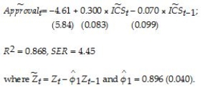 How is this equation related to the ones in (a)and (b)? What are the properties of the GLS estimator here,under the assumption that ICS is strictly exogenous?
(d)Is it likely that the ICS is exogenous here? Strictly exogenous?
You want to see how this approval rating is related to the Michigan index of consumer sentiment (ICS).The monthly survey,conducted with a minimum sample of 500,asks people if they feel "better/worse off" with regard to current and future conditions.
(a)To estimate dynamic causal effects,you collect quarterly data from 1962:I - 1998:II for the United States.You allow a binary variable for each presidency to capture the intrinsic popularity of the President.Furthermore,you eliminate observations that include a change in party for the presidency by using a binary variable,which takes on the value of one during the first quarter of the year after the election.Finally,a friendly political scientist provides you with (i)an "events" variable, (ii)a "Vietnam" binary variable,and (iii)a "honeymoon" variable,which measures the effect of a higher popularity of a president immediately following the election.(The coefficients of these variables will not be reported here. )
Assuming that consumer sentiment is exogenous,you estimate the following two specifications (numbers in parenthesis are heteroskedasticity- and autocorrelation-consistent standard errors):
t = 26.08 + 0.178 × ICSt + 0.232 × ICSt-1;R2= 0.667,SER = 7.00(8.83)(0.120)(0.135)
t = 26.08 + 0.178 × ΔICSt + 0.411 + ICSt-1;R2 = 0.667,SER = 7.00(8.17)(0.120 )(0.089)
What is the difference between the two specifications? What is the advantage of estimating the second equation,if any?
(b)Assuming that the errors follow an AR(1)process,you also estimate the following alternative:
t = -4.61 + 0.300 × ICSt - 0.070 × ICSt-1- 0.054 × ICSt-2;+ 0.776 × Approvalt-1;(5.84)(0.083)(0.099)(0.083)(0.057)
R2 = 0.868,SER = 4.45
How is this specification related to the previous ones? What implicit assumptions did you have to make to allow for desirable properties of the OLS estimator?
(c)You finally estimate the approval equation using the quasi-difference specification and the GLS estimator.
How is this equation related to the ones in (a)and (b)? What are the properties of the GLS estimator here,under the assumption that ICS is strictly exogenous?(d)Is it likely that the ICS is exogenous here? Strictly exogenous?
سؤال
سؤال
سؤال
سؤال
سؤال
One of the central predictions of neo-classical macroeconomic growth theory is that an increase in the growth rate of the population causes at first a decline the growth rate of real output per capita,but that subsequently the growth rate returns to its natural level,itself determined by the rate of technological innovation.The intuition is that,if the growth rate of the workforce increases,then more has to be saved to provide the new workers with physical capital.However,accumulating capital takes time,so that output per capita falls in the short run.
Under the assumption that population growth is exogenous,a number of regressions of the growth rate of output per capita on current and lagged population growth were performed,as reported below.(A constant was included in the regressions but is not reported.HAC standard errors are in brackets.BIC is listed at the bottom of the table).
Regression of Growth Rate of Real Per-Capita GDP on Lags of Population Growth,
United States,1825-2000
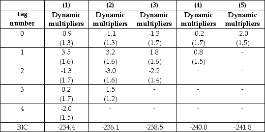 (a)Which of these models is favored by the information criterion?
(b)How consistent are these estimates with the theory? Is this a fair test of the theory? Why or why not?
(c)Can you think of any improved data to test the theory?
Under the assumption that population growth is exogenous,a number of regressions of the growth rate of output per capita on current and lagged population growth were performed,as reported below.(A constant was included in the regressions but is not reported.HAC standard errors are in brackets.BIC is listed at the bottom of the table).
Regression of Growth Rate of Real Per-Capita GDP on Lags of Population Growth,
United States,1825-2000
(a)Which of these models is favored by the information criterion?(b)How consistent are these estimates with the theory? Is this a fair test of the theory? Why or why not?
(c)Can you think of any improved data to test the theory?
سؤال
سؤال
The distributed lag model assumptions include all of the following with the exception of:
A)There is no perfect multicollinearity.
B)Xt is strictly exogenous.
C)E(ut Xt,Xt-1,Xt-2)= 0
D)The random variables Xt and Yt have a stationary distribution.
A)There is no perfect multicollinearity.
B)Xt is strictly exogenous.
C)E(ut
Xt,Xt-1,Xt-2)= 0D)The random variables Xt and Yt have a stationary distribution.
سؤال
سؤال
سؤال
سؤال
(Requires Appendix material)Your textbook states that in "the distributed lag regression model,the error term ut can be correlated with its lagged values.This autocorrelation arises,because,in time series data,the omitted factors that comprise ut can themselves be serially correlated."
(a)Give an example what the authors have in mind.
(b)Consider the ADL model,where the X's are strictly exogenous,and there is no autocorrelation (and/or heteroskedasticity)in the error term.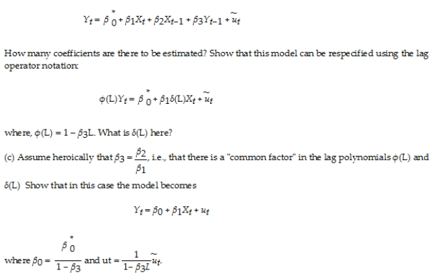 (d)Explain why autocorrelation in this model can be seen as a "simplification," not a "nuisance." Can you use the F-test to test the above hypothesis? Why or why not?
(a)Give an example what the authors have in mind.
(b)Consider the ADL model,where the X's are strictly exogenous,and there is no autocorrelation (and/or heteroskedasticity)in the error term.
(d)Explain why autocorrelation in this model can be seen as a "simplification," not a "nuisance." Can you use the F-test to test the above hypothesis? Why or why not? سؤال
It has been argued that Canada's aggregate output growth and unemployment rates are very sensitive to United States economic fluctuations,while the opposite is not true.
(a)A researcher uses a distributed lag model to estimate dynamic causal effects of U.S.economic activity on Canada.The results (HAC standard errors in parenthesis)for the sample period 1961:I-1995:IV are: t = -1.42 + 0.717 × urust + 0.262 × urust-1 + 0.023 × urust-2 - 0.083 × urust-3
(0.83)(0.457)(0.557)(0.398)(0.405)
- 0.726 × urust-4 + 1.267 × urust-5;R2= 0.672,SER = 1.444
(0.504)(0.385)
where urcan is the Canadian unemployment rate,and urus is the United States unemployment rate.
Calculate the long-run cumulative dynamic multiplier.
(b)What are some of the omitted variables that could cause autocorrelation in the error terms? Are these omitted variables likely to uncorrelated with current and lagged values of the U.S.unemployment rate? Do you think that the U.S.unemployment rate is exogenous in this distributed lag regression?
(a)A researcher uses a distributed lag model to estimate dynamic causal effects of U.S.economic activity on Canada.The results (HAC standard errors in parenthesis)for the sample period 1961:I-1995:IV are:
t = -1.42 + 0.717 × urust + 0.262 × urust-1 + 0.023 × urust-2 - 0.083 × urust-3(0.83)(0.457)(0.557)(0.398)(0.405)
- 0.726 × urust-4 + 1.267 × urust-5;R2= 0.672,SER = 1.444
(0.504)(0.385)
where urcan is the Canadian unemployment rate,and urus is the United States unemployment rate.
Calculate the long-run cumulative dynamic multiplier.
(b)What are some of the omitted variables that could cause autocorrelation in the error terms? Are these omitted variables likely to uncorrelated with current and lagged values of the U.S.unemployment rate? Do you think that the U.S.unemployment rate is exogenous in this distributed lag regression?
سؤال
سؤال
You are hired to forecast the unemployment rate in a geographical area that is peripheral to a large metropolitan area in the United States.The area in question is called the Inland Empire (San Bernardino County and Riverside County)and is situated east of Greater Los Angeles (Los Angeles County and Orange County).While the area has a large population (it is the 14th largest metropolitan statistical area in the United States),its economic activity relies heavily on that of the larger area it is attached to.For example,it is estimated that approximately 20% of its workforce commutes into the Greater Los Angeles area for work and few workers commute the other way.Furthermore,its logistics industry is heavily dependent on economic activity in the Greater Los Angeles Area.As a result,you view the unemployment rate of the Greater Los Angeles Area (urGLA)to be exogenous in determining the unemployment rate in the Inland Empire (urIE).You estimate the following distributed lag model,where numbers in parenthesis are HAC standard errors:
Δ = 0.00002 + 0.74 Δ
  - 0.04 Δ
  - 0.01 Δ
  + 0.07 Δ
  + 0.05 Δ
  (0.00010)(0.06)(0.06)(0.06)(0.06)(0.06)
+ 0.09 Δ + 0.10Δ
  (0.05)(0.06)
t = 1991:01-2009:12,R2 = 0.60,SER = 0.001
a.What is the impact effect of a one percentage point increase (say from 0.06 to 0.07)of the unemployment rate in the Greater Los Angeles area?
b.What is the long-run cumulative dynamic multiplier?
c.Why do you think the variables above appear in changes rather than in levels?
Δ
= 0.00002 + 0.74 Δ - 0.04 Δ - 0.01 Δ + 0.07 Δ + 0.05 Δ (0.00010)(0.06)(0.06)(0.06)(0.06)(0.06)+ 0.09 Δ
+ 0.10Δ (0.05)(0.06)t = 1991:01-2009:12,R2 = 0.60,SER = 0.001
a.What is the impact effect of a one percentage point increase (say from 0.06 to 0.07)of the unemployment rate in the Greater Los Angeles area?
b.What is the long-run cumulative dynamic multiplier?
c.Why do you think the variables above appear in changes rather than in levels?
سؤال
There is some economic research which suggests that oil prices play a central role in causing recessions in developed countries.Some of this work suggests that it is only oil price increases that matter and even more specifically,that it is the percentage point difference between oil prices at date t and the maximum value over the previous year.Realizing that energy prices in general can fluctuate quite dramatically in both directions and that geographic areas also benefit substantially from oil price decreases,you decide to estimate the following distributed lag model using annual data (numbers in parenthesis are HAC standard errors):  t = 3.39 - 0.009 (Poil/CPI)t - 0.028 (Poil/CPI)t-1
(0.27)(0.010)(0.011)
t = 1960-2008,R2 = 0.15,SER = 1.88
a.What is the impact effect of a 25 percent increase in real oil prices?
b.What is the predicted cumulative change in GDP Growth over two years of this effect?
c.The HAC F-statistic is 4.07.Can you reject the null hypothesis that oil price changes have no effect on real GDP growth? What is the critical value you considered? Is there any reason why you should be cautious using an F-test in this case,given the sample period?
t = 3.39 - 0.009 (Poil/CPI)t - 0.028 (Poil/CPI)t-1(0.27)(0.010)(0.011)
t = 1960-2008,R2 = 0.15,SER = 1.88
a.What is the impact effect of a 25 percent increase in real oil prices?
b.What is the predicted cumulative change in GDP Growth over two years of this effect?
c.The HAC F-statistic is 4.07.Can you reject the null hypothesis that oil price changes have no effect on real GDP growth? What is the critical value you considered? Is there any reason why you should be cautious using an F-test in this case,given the sample period?
سؤال
سؤال
Your textbook estimates the initial relationship between the percentage change of real frozen OJ and the freezing degree days as follows:  t = -0.40 + 0.47 FDDt
(0.22)(0.13)
t = 1950:1 - 2000:12,R2 = 0.09,SER = 4.8
a.Calculate the t-statistic for the slope coefficient.Can you reject the null hypothesis that the coefficient is zero in the population?
b.The above regression was estimated using HAC standard errors.When you re-estimate the regression using homoskedasticity-only standard errors,the standard error of the slope coefficient drops to 0.06.Calculate the t-statistic for the slope coefficient again.Which of the two standard errors should you use for statistical inference?
t = -0.40 + 0.47 FDDt(0.22)(0.13)
t = 1950:1 - 2000:12,R2 = 0.09,SER = 4.8
a.Calculate the t-statistic for the slope coefficient.Can you reject the null hypothesis that the coefficient is zero in the population?
b.The above regression was estimated using HAC standard errors.When you re-estimate the regression using homoskedasticity-only standard errors,the standard error of the slope coefficient drops to 0.06.Calculate the t-statistic for the slope coefficient again.Which of the two standard errors should you use for statistical inference?
سؤال
Your textbook used a distributed lag model with only current and past values of Xt-1 coupled with an AR(1)error model to derive a quasi-difference model,where the error term was uncorrelated.
(a)Instead use a static model Yt = β0 + β1Xt + ut here,where the error term follows an AR(1).Derive the quasi difference form.Explain why in the case of the infeasible GLS estimators you could easily estimate the βs by OLS.
(b)Since φ1 (the autocorrelation parameter for ut)is unknown,describe the Cochrane-Orcutt estimation procedure.
(c)Explain how the iterated Cochrane-Orcutt estimator works in this situation.Iterations stop when there is "convergence" in the estimates.What do you think is meant by that?
(d)Your textbook has pointed out that the iterated Cochrane-Orcutt GLS estimator is in fact the nonlinear least squares estimator of the model.Given that -1 < φ1 < 1,suggest a "grid search" or some strategy to "nail down" the value of 1 which minimizes the sum of squared residuals.This is the so-called Hildreth-Lu method.
(a)Instead use a static model Yt = β0 + β1Xt + ut here,where the error term follows an AR(1).Derive the quasi difference form.Explain why in the case of the infeasible GLS estimators you could easily estimate the βs by OLS.
(b)Since φ1 (the autocorrelation parameter for ut)is unknown,describe the Cochrane-Orcutt estimation procedure.
(c)Explain how the iterated Cochrane-Orcutt estimator works in this situation.Iterations stop when there is "convergence" in the estimates.What do you think is meant by that?
(d)Your textbook has pointed out that the iterated Cochrane-Orcutt GLS estimator is in fact the nonlinear least squares estimator of the model.Given that -1 < φ1 < 1,suggest a "grid search" or some strategy to "nail down" the value of
1 which minimizes the sum of squared residuals.This is the so-called Hildreth-Lu method. سؤال
Consider the following model Yt = β0 +  + ut where the superscript "e" indicates expected values.This may represent an example where consumption depends on expected,or "permanent," income.Furthermore,let expected income be formed as follows:
  =
=  + λ(Xt -
  );0 < λ < 1
(a)In the above expectation formation hypothesis,expectations are formed at the end of the period,say the 31st of December,if you had annual data.Give an intuitive explanation for this process.
(b)Rewrite the expectations equation in the following form: = (1 - λ)
  + λXt
+ λXt
Next,following the method used in your textbook,lag both sides of the equation and replace .Repeat this process by repeatedly substituting expression for
  ,
,  ,and so forth.Show that this results in the following equation:
  = λXt + λ(1-λ)Xt-1 + λ(1- λ)2 Xt-2 + ...+ λ(1- λ)n Xt-n + (1 - λ)n+1
  Explain why it is reasonable to drop the last right hand side term as n becomes large.
(c)Substitute the above expression into the original model that related Y to .Although you now have right hand side variables that are all observable,what do you perceive as a potential problem here if you wanted to estimate this distributed lag model without further restrictions?
(d)Lag both sides of the equation,multiply through by (1- λ),and subtract this equation from the equation found in (c).This is called a "Koyck transformation." What does the resulting equation look like? What is the error process? What is the impact effect (zero-period dynamic multiplier)of a unit change in X,and how does it differ from long run cumulative dynamic multiplier?
+ ut where the superscript "e" indicates expected values.This may represent an example where consumption depends on expected,or "permanent," income.Furthermore,let expected income be formed as follows: = + λ(Xt - );0 < λ < 1(a)In the above expectation formation hypothesis,expectations are formed at the end of the period,say the 31st of December,if you had annual data.Give an intuitive explanation for this process.
(b)Rewrite the expectations equation in the following form:
= (1 - λ) + λXtNext,following the method used in your textbook,lag both sides of the equation and replace
.Repeat this process by repeatedly substituting expression for , ,and so forth.Show that this results in the following equation: = λXt + λ(1-λ)Xt-1 + λ(1- λ)2 Xt-2 + ...+ λ(1- λ)n Xt-n + (1 - λ)n+1 Explain why it is reasonable to drop the last right hand side term as n becomes large.(c)Substitute the above expression into the original model that related Y to
.Although you now have right hand side variables that are all observable,what do you perceive as a potential problem here if you wanted to estimate this distributed lag model without further restrictions?(d)Lag both sides of the equation,multiply through by (1- λ),and subtract this equation from the equation found in (c).This is called a "Koyck transformation." What does the resulting equation look like? What is the error process? What is the impact effect (zero-period dynamic multiplier)of a unit change in X,and how does it differ from long run cumulative dynamic multiplier?
سؤال

فتح الحزمة
قم بالتسجيل لفتح البطاقات في هذه المجموعة!
Unlock Deck
Unlock Deck
1/50
العب
ملء الشاشة (f)
Deck 15: Estimation of Dynamic Causal Effects
1
A distributed lag regression
A)is also called AR(p).
B)can also be used with cross-sectional data.
C)gives estimates of dynamic causal effects.
D)is sometimes referred to as ADL.
A)is also called AR(p).
B)can also be used with cross-sectional data.
C)gives estimates of dynamic causal effects.
D)is sometimes referred to as ADL.
C
2
To convey information about the dynamic multipliers more effectively,you should
A)plot them.
B)discuss these carefully one at a time.
C)estimate them by maximum likelihood methods.
D)first make sure that they are stationary.
A)plot them.
B)discuss these carefully one at a time.
C)estimate them by maximum likelihood methods.
D)first make sure that they are stationary.
A
3
The concept of exogeneity is important because
A)it clarifies whether or not the variable is determined inside or outside your model.
B)maximum likelihood estimation is no longer valid.
C)under strict exogeneity,OLS may not be efficient as an estimator of dynamic causal effects.
D)endogenous variables are not stationary,but exogenous variables are.
C
4
Infeasible GLS
A)requires too much memory even for today's PCs.
B)uses complicated interative techniques.
C)cannot be calculated since it also uses quasi differences for Xt.
D)assumes the parameters of the error autocorrelation process to be known.
A)requires too much memory even for today's PCs.
B)uses complicated interative techniques.
C)cannot be calculated since it also uses quasi differences for Xt.
D)assumes the parameters of the error autocorrelation process to be known.
فتح الحزمة
افتح القفل للوصول البطاقات البالغ عددها 50 في هذه المجموعة.
فتح الحزمة
k this deck
5
Sensitivity analysis of the results may include the following with the exception of
A)stability over time analysis of the estimated multipliers.
B)using homoskedasticity only rather than HAC standard errors.
C)investigation of omitted variable bias.
D)looking at different computations of the HAC standard errors.
A)stability over time analysis of the estimated multipliers.
B)using homoskedasticity only rather than HAC standard errors.
C)investigation of omitted variable bias.
D)looking at different computations of the HAC standard errors.
فتح الحزمة
افتح القفل للوصول البطاقات البالغ عددها 50 في هذه المجموعة.
فتح الحزمة
k this deck
6
GLS involves
A)writing the model in differences and estimating it by OLS,using HAC standard errors.
B)truncating the sample at both ends of the period,then estimating by OLS using HAC standard errors.
C)checking the AIC rather than the BIC in choosing the maximum lag-length of the regressors.
D)transforming the regression model so that the errors are homoskedastic and serially uncorrelated,and then estimating the transformed regression model by OLS.
فتح الحزمة
افتح القفل للوصول البطاقات البالغ عددها 50 في هذه المجموعة.
فتح الحزمة
k this deck
7
Ascertaining whether or not a regressor is strictly exogenous or exogenous ultimately requires all of the following with the exception of
A)economic theory.
B)institutional knowledge.
C)expert judgment.
D)use of HAC standard errors.
A)economic theory.
B)institutional knowledge.
C)expert judgment.
D)use of HAC standard errors.
فتح الحزمة
افتح القفل للوصول البطاقات البالغ عددها 50 في هذه المجموعة.
فتح الحزمة
k this deck
8
GLS
A)results in smaller variances of the estimator than OLS if the regressors are strictly exogenous.
B)is the same as OLS using HAC standard errors.
C)can be used even if the regressors are not strictly exogenous.
D)can be used for time-series estimation,but not in cross-sectional data.
A)results in smaller variances of the estimator than OLS if the regressors are strictly exogenous.
B)is the same as OLS using HAC standard errors.
C)can be used even if the regressors are not strictly exogenous.
D)can be used for time-series estimation,but not in cross-sectional data.
فتح الحزمة
افتح القفل للوصول البطاقات البالغ عددها 50 في هذه المجموعة.
فتح الحزمة
k this deck
9
In time series,the definition of causal effects
A)says that one variable helps predict another variable.
B)does not make much sense since there are not multiple subjects.
C)assumes that the same subject is being given different treatments at different points in time.
D)requires panel data.
A)says that one variable helps predict another variable.
B)does not make much sense since there are not multiple subjects.
C)assumes that the same subject is being given different treatments at different points in time.
D)requires panel data.
فتح الحزمة
افتح القفل للوصول البطاقات البالغ عددها 50 في هذه المجموعة.
فتح الحزمة
k this deck
10
A seasonal binary (or indicator or dummy)variable,in the case of monthly data,
A)is a binary variable that take on the value of 1 for a given month and is 0 otherwise.
B)is a variable that has values of 1 to 12 in a given year.
C)is a variable that contains 1s during a given year and is 0 otherwise.
D)does not exist,since a month is not a season.
A)is a binary variable that take on the value of 1 for a given month and is 0 otherwise.
B)is a variable that has values of 1 to 12 in a given year.
C)is a variable that contains 1s during a given year and is 0 otherwise.
D)does not exist,since a month is not a season.
فتح الحزمة
افتح القفل للوصول البطاقات البالغ عددها 50 في هذه المجموعة.
فتح الحزمة
k this deck
11
The distributed lag model is given by
A)Yt = β0 + β1Xt + β2Yt-1 + ut.
B)Yt = β0 + β1Yt-1 + β2Yt-2 + ...+ βrYt-r + ut.
C)Yt = β0 + β1ut + β2ut+1 + β3ut+2 + ...+ βr+1ut+r + et.
D)Yt = β0 + β1Xt + β2Xt-1 + β3Xt-2 + ...+ βr+1Xt-r + ut.
A)Yt = β0 + β1Xt + β2Yt-1 + ut.
B)Yt = β0 + β1Yt-1 + β2Yt-2 + ...+ βrYt-r + ut.
C)Yt = β0 + β1ut + β2ut+1 + β3ut+2 + ...+ βr+1ut+r + et.
D)Yt = β0 + β1Xt + β2Xt-1 + β3Xt-2 + ...+ βr+1Xt-r + ut.
فتح الحزمة
افتح القفل للوصول البطاقات البالغ عددها 50 في هذه المجموعة.
فتح الحزمة
k this deck
12
Autocorrelation of the error terms
A)makes it impossible to calculate homoskedasticity only standard errors.
B)causes OLS to be no longer consistent.
C)causes the usual OLS standard errors to be inconsistent.
D)results in OLS being biased.
A)makes it impossible to calculate homoskedasticity only standard errors.
B)causes OLS to be no longer consistent.
C)causes the usual OLS standard errors to be inconsistent.
D)results in OLS being biased.
فتح الحزمة
افتح القفل للوصول البطاقات البالغ عددها 50 في هذه المجموعة.
فتح الحزمة
k this deck
13
Heteroskedasticity- and autocorrelation-consistent standard errors
A)result in the OLS estimator being BLUE.
B)should be used when errors are autocorrelated.
C)are calculated when using the Cochrane-Orcutt iterative procedure.
D)have the same formula as the heteroskedasticity robust standard errors in cross-sections.
A)result in the OLS estimator being BLUE.
B)should be used when errors are autocorrelated.
C)are calculated when using the Cochrane-Orcutt iterative procedure.
D)have the same formula as the heteroskedasticity robust standard errors in cross-sections.
فتح الحزمة
افتح القفل للوصول البطاقات البالغ عددها 50 في هذه المجموعة.
فتح الحزمة
k this deck
14
The 95% confidence interval for the dynamic multipliers should be computed by using the estimated coefficient ±
A)1.96 times the RMSFE.
B)1.96 times the HAC standard errors.
C)1.96,since the HAC errors are standardized.
D)1.64 times the HAC standard errors since the alternative hypothesis is one-sided.
A)1.96 times the RMSFE.
B)1.96 times the HAC standard errors.
C)1.96,since the HAC errors are standardized.
D)1.64 times the HAC standard errors since the alternative hypothesis is one-sided.
فتح الحزمة
افتح القفل للوصول البطاقات البالغ عددها 50 في هذه المجموعة.
فتح الحزمة
k this deck
15
The impact effect is the
A)zero period dynamic multiplier.
B)h period dynamic multiplier,h>0.
C)cumulative dynamic multiplier.
D)long-run cumulative dynamic multiplier.
A)zero period dynamic multiplier.
B)h period dynamic multiplier,h>0.
C)cumulative dynamic multiplier.
D)long-run cumulative dynamic multiplier.
فتح الحزمة
افتح القفل للوصول البطاقات البالغ عددها 50 في هذه المجموعة.
فتح الحزمة
k this deck
16
The concepts of exogeneity,strict exogeneity,and predeterminedness
A)are defined in such a way that strict exogeneity implies exogeneity.
B)can be used interchangeably.
C)are defined in such a way that exogeneity implies strict exogeneity.
D)correspond to endogeneity,strict endogeneity,and lagged endogenous variables.
A)are defined in such a way that strict exogeneity implies exogeneity.
B)can be used interchangeably.
C)are defined in such a way that exogeneity implies strict exogeneity.
D)correspond to endogeneity,strict endogeneity,and lagged endogenous variables.
فتح الحزمة
افتح القفل للوصول البطاقات البالغ عددها 50 في هذه المجموعة.
فتح الحزمة
k this deck
17
The long-run cumulative dynamic multiplier
A)cannot be calculated since in the long-run,we are all dead.
B)is the sum of all individual dynamic multipliers.
C)is the coefficient on Xt-r in the standard formulation of the distributed lag model.
D)is the difference between the coefficient on Xt-1 and Xt-r.
A)cannot be calculated since in the long-run,we are all dead.
B)is the sum of all individual dynamic multipliers.
C)is the coefficient on Xt-r in the standard formulation of the distributed lag model.
D)is the difference between the coefficient on Xt-1 and Xt-r.
فتح الحزمة
افتح القفل للوصول البطاقات البالغ عددها 50 في هذه المجموعة.
فتح الحزمة
k this deck
18
Estimation of dynamic multipliers under strict exogeneity should be done by
A)instrumental variable methods.
B)OLS.
C)feasible GLS.
D)analyzing the stationarity of the multipliers.
A)instrumental variable methods.
B)OLS.
C)feasible GLS.
D)analyzing the stationarity of the multipliers.
فتح الحزمة
افتح القفل للوصول البطاقات البالغ عددها 50 في هذه المجموعة.
فتح الحزمة
k this deck
19
Quasi differences in Yt are defined as
A)Yt - Yt-1.
B)Yt - φ1Yt-1.
C)△Yt - φ1Yt-1.
D)φ1(Yt - Yt-1).
A)Yt - Yt-1.
B)Yt - φ1Yt-1.
C)△Yt - φ1Yt-1.
D)φ1(Yt - Yt-1).
فتح الحزمة
افتح القفل للوصول البطاقات البالغ عددها 50 في هذه المجموعة.
فتح الحزمة
k this deck
20
The Cochrane-Orcutt iterative method is
A)a special case of GLS estimation.
B)a method to compute HAC standard errors.
C)a special case of maximum likelihood estimation.
D)a grid search for the autoregressive parameters on the error process.
A)a special case of GLS estimation.
B)a method to compute HAC standard errors.
C)a special case of maximum likelihood estimation.
D)a grid search for the autoregressive parameters on the error process.
فتح الحزمة
افتح القفل للوصول البطاقات البالغ عددها 50 في هذه المجموعة.
فتح الحزمة
k this deck
21
Consider the distributed lag model Yt = β0 + β1Xt + β2Xt-1 + β3Xt-2 + … + βr+1Xt-r + ut.The dynamic causal effect is
A)β0 + β1
B)β1 + β2+…+βr+1
C)β0 + β1+…+βr+1
D)β1
A)β0 + β1
B)β1 + β2+…+βr+1
C)β0 + β1+…+βr+1
D)β1
فتح الحزمة
افتح القفل للوصول البطاقات البالغ عددها 50 في هذه المجموعة.
فتح الحزمة
k this deck
22
Given the relationship between the two variables,the following is most likely to be exogenous:
A)the inflation rate and the short term interest rate: short-term interest rate is exogenous
B)U.S.rate of inflation and increases in oil prices: oil prices are exgoneous
C)Australian exports and U.S.aggregate income: U.S.aggregate income is exogenous
D)change in inflation,lagged changes of inflation,and lags of unemployment: lags of unemployment are exogenous
فتح الحزمة
افتح القفل للوصول البطاقات البالغ عددها 50 في هذه المجموعة.
فتح الحزمة
k this deck
23
GLS is consistent and BLUE if
A)X is predetermined.
B)the error process is AR(1).
C)X is strictly exogenous.
D)all the roots are inside the unit circle.
A)X is predetermined.
B)the error process is AR(1).
C)X is strictly exogenous.
D)all the roots are inside the unit circle.
فتح الحزمة
افتح القفل للوصول البطاقات البالغ عددها 50 في هذه المجموعة.
فتح الحزمة
k this deck
24
A model that attracted quite a bit of interest in macroeconomics in the 1970s was the St.Louis model.The underlying idea was to calculate fiscal and monetary impact and long run cumulative dynamic multipliers,by relating output (growth)to government expenditure (growth)and money supply (growth).The assumption was that both government expenditures and the money supply were exogenous.Estimation of a St.Louis type model using quarterly data from 1960:I-1995:IV results in the following output (HAC standard errors in parenthesis): t = 0.018 + 0.006 × dmgrowtht + 0.235 × dmgrowtht-1 + 0.344 × dmgrowtht-2
(0.004)(0.079)(0.091)(0.087)
+ 0.385 × dmgrotht-3 + 0.425 × mgrowtht-4 + 0.170 × dggrowtht - 0.044dggrowtht-1
(0.097)(0.069)(0.049)(0.068)
- 0.003 × dggrowtht-2 - 0.079 × dggrowtht-3 + 0.018 × ggrowtht-4;
(0.040)(0.051)(0.027)
R2 = 0.346,SER=0.03
where ygrowth is quarterly growth of real GDP,mgrowth is quarterly growth of real money supply (M2),and ggrowth is quarterly growth of real government expenditures."d" in front of ggrowth and mgrowth indicates a change in the variable.
(a)Assuming that money and government expenditures are exogenous,what do the coefficients represent? Calculate the h-period cumulative dynamic multipliers from these.How can you test for the statistical significance of the cumulative dynamic multipliers and the long-run cumulative dynamic multiplier?
(b)Sketch the estimated dynamic and cumulative dynamic fiscal and monetary multipliers.
(c)For these coefficients to represent dynamic multipliers,the money supply and government expenditures must be exogenous variables.Explain why this is unlikely to be the case.As a result,what importance should you attach to the above results?
t = 0.018 + 0.006 × dmgrowtht + 0.235 × dmgrowtht-1 + 0.344 × dmgrowtht-2(0.004)(0.079)(0.091)(0.087)
+ 0.385 × dmgrotht-3 + 0.425 × mgrowtht-4 + 0.170 × dggrowtht - 0.044dggrowtht-1
(0.097)(0.069)(0.049)(0.068)
- 0.003 × dggrowtht-2 - 0.079 × dggrowtht-3 + 0.018 × ggrowtht-4;
(0.040)(0.051)(0.027)
R2 = 0.346,SER=0.03
where ygrowth is quarterly growth of real GDP,mgrowth is quarterly growth of real money supply (M2),and ggrowth is quarterly growth of real government expenditures."d" in front of ggrowth and mgrowth indicates a change in the variable.
(a)Assuming that money and government expenditures are exogenous,what do the coefficients represent? Calculate the h-period cumulative dynamic multipliers from these.How can you test for the statistical significance of the cumulative dynamic multipliers and the long-run cumulative dynamic multiplier?
(b)Sketch the estimated dynamic and cumulative dynamic fiscal and monetary multipliers.
(c)For these coefficients to represent dynamic multipliers,the money supply and government expenditures must be exogenous variables.Explain why this is unlikely to be the case.As a result,what importance should you attach to the above results?
فتح الحزمة
افتح القفل للوصول البطاقات البالغ عددها 50 في هذه المجموعة.
فتح الحزمة
k this deck
25
In your intermediate macroeconomics course,government expenditures and the money supply were treated as exogenous,in the sense that the variables could be changed to conduct economic policy to influence target variables,but that these variables would not react to changes in the economy as a result of some fixed rule.The St.Louis Model,proposed by two researchers at the Federal Reserve in St.Louis,used this idea to test whether monetary policy or fiscal policy was more effective in influencing output behavior.Although there were various versions of this model,the basic specification was of the following type:
Δln(Yt)= β0 + β1Δln mt + ...+ βpΔln mt-p-1 + βp+1Δln Gt + ...+ βp+qΔln Gt-q-1 + ut
Assuming that money supply and government expenditures are exogenous,how would you estimate dynamic causal effects? Why do you think this type of model is no longer used by most to calculate fiscal and monetary multipliers?
فتح الحزمة
افتح القفل للوصول البطاقات البالغ عددها 50 في هذه المجموعة.
فتح الحزمة
k this deck
26
In the distributed lag model,the coefficient on the contemporaneous value of the regressor is called the
A)dynamic effect.
B)cumulative multiplier.
C)autoregressive error.
D)impact effect.
A)dynamic effect.
B)cumulative multiplier.
C)autoregressive error.
D)impact effect.
فتح الحزمة
افتح القفل للوصول البطاقات البالغ عددها 50 في هذه المجموعة.
فتح الحزمة
k this deck
27
HAC standard errors should be used because
A)they are convenient simplifications of the heteroskedasticity-robust standard errors.
B)conventional standard errors may result in misleading inference.
C)they are easier to calculate than the heteroskedasticity-robust standard errors and yet still allow you to perform inference correctly.
D)when there is a structural break,then conventional standard errors result in misleading inference.
فتح الحزمة
افتح القفل للوصول البطاقات البالغ عددها 50 في هذه المجموعة.
فتح الحزمة
k this deck
28
Consider the following distributed lag model is serially uncorrelated,and X is strictly exogenous.
(a)How many parameters are there to be estimated between the two equations?
(b)Using the two equations of the model above,derive the ADL form of the model.
(c)There are five regressors in the ADL model,namely Yt-1,Xt,Xt-1,Xt-2 and the constant.Estimating the ADL model linearly will give you five coefficients.Can you derive the parameters of the original two equation model from these five estimates? Why or why not?
(d)What alternative method do you have to retrieve the parameters of the two equation model?
is serially uncorrelated,and X is strictly exogenous.(a)How many parameters are there to be estimated between the two equations?
(b)Using the two equations of the model above,derive the ADL form of the model.
(c)There are five regressors in the ADL model,namely Yt-1,Xt,Xt-1,Xt-2 and the constant.Estimating the ADL model linearly will give you five coefficients.Can you derive the parameters of the original two equation model from these five estimates? Why or why not?
(d)What alternative method do you have to retrieve the parameters of the two equation model?
فتح الحزمة
افتح القفل للوصول البطاقات البالغ عددها 50 في هذه المجموعة.
فتح الحزمة
k this deck
29
Your textbook presents as an example of a distributed lag regression the effect of the weather on the price of orange juice.The authors mention U.S.income and Australian exports,oil prices and inflation,monetary policy and inflation,and the Phillips curve as other candidates for distributed lag regression.Briefly discuss whether or not the exogeneity assumption is likely to hold in each of these cases.Explain why it is so hard to come up with good examples of distributed lag regressions in economics.
فتح الحزمة
افتح القفل للوصول البطاقات البالغ عددها 50 في هذه المجموعة.
فتح الحزمة
k this deck
30
The Gallup Poll frequently surveys the electorate to quantify the public's opinion of the president.Since 1945,Gallup settled on the following wording of its presidential poll: "Do you approve or disapprove of the way (name)is handling his job as president?" Gallup has not changed its presidential question since then,and respondents can answer "approve," "disapprove," or "no opinion."
You want to see how this approval rating is related to the Michigan index of consumer sentiment (ICS).The monthly survey,conducted with a minimum sample of 500,asks people if they feel "better/worse off" with regard to current and future conditions.
(a)To estimate dynamic causal effects,you collect quarterly data from 1962:I - 1998:II for the United States.You allow a binary variable for each presidency to capture the intrinsic popularity of the President.Furthermore,you eliminate observations that include a change in party for the presidency by using a binary variable,which takes on the value of one during the first quarter of the year after the election.Finally,a friendly political scientist provides you with (i)an "events" variable, (ii)a "Vietnam" binary variable,and (iii)a "honeymoon" variable,which measures the effect of a higher popularity of a president immediately following the election.(The coefficients of these variables will not be reported here. )
Assuming that consumer sentiment is exogenous,you estimate the following two specifications (numbers in parenthesis are heteroskedasticity- and autocorrelation-consistent standard errors): t = 26.08 + 0.178 × ICSt + 0.232 × ICSt-1;R2= 0.667,SER = 7.00
(8.83)(0.120)(0.135) t = 26.08 + 0.178 × ΔICSt + 0.411 + ICSt-1;R2 = 0.667,SER = 7.00
(8.17)(0.120 )(0.089)
What is the difference between the two specifications? What is the advantage of estimating the second equation,if any?
(b)Assuming that the errors follow an AR(1)process,you also estimate the following alternative: t = -4.61 + 0.300 × ICSt - 0.070 × ICSt-1- 0.054 × ICSt-2;+ 0.776 × Approvalt-1;
(5.84)(0.083)(0.099)(0.083)(0.057)
R2 = 0.868,SER = 4.45
How is this specification related to the previous ones? What implicit assumptions did you have to make to allow for desirable properties of the OLS estimator?
(c)You finally estimate the approval equation using the quasi-difference specification and the GLS estimator. How is this equation related to the ones in (a)and (b)? What are the properties of the GLS estimator here,under the assumption that ICS is strictly exogenous?
(d)Is it likely that the ICS is exogenous here? Strictly exogenous?
You want to see how this approval rating is related to the Michigan index of consumer sentiment (ICS).The monthly survey,conducted with a minimum sample of 500,asks people if they feel "better/worse off" with regard to current and future conditions.
(a)To estimate dynamic causal effects,you collect quarterly data from 1962:I - 1998:II for the United States.You allow a binary variable for each presidency to capture the intrinsic popularity of the President.Furthermore,you eliminate observations that include a change in party for the presidency by using a binary variable,which takes on the value of one during the first quarter of the year after the election.Finally,a friendly political scientist provides you with (i)an "events" variable, (ii)a "Vietnam" binary variable,and (iii)a "honeymoon" variable,which measures the effect of a higher popularity of a president immediately following the election.(The coefficients of these variables will not be reported here. )
Assuming that consumer sentiment is exogenous,you estimate the following two specifications (numbers in parenthesis are heteroskedasticity- and autocorrelation-consistent standard errors):
t = 26.08 + 0.178 × ICSt + 0.232 × ICSt-1;R2= 0.667,SER = 7.00(8.83)(0.120)(0.135)
t = 26.08 + 0.178 × ΔICSt + 0.411 + ICSt-1;R2 = 0.667,SER = 7.00(8.17)(0.120 )(0.089)
What is the difference between the two specifications? What is the advantage of estimating the second equation,if any?
(b)Assuming that the errors follow an AR(1)process,you also estimate the following alternative:
t = -4.61 + 0.300 × ICSt - 0.070 × ICSt-1- 0.054 × ICSt-2;+ 0.776 × Approvalt-1;(5.84)(0.083)(0.099)(0.083)(0.057)
R2 = 0.868,SER = 4.45
How is this specification related to the previous ones? What implicit assumptions did you have to make to allow for desirable properties of the OLS estimator?
(c)You finally estimate the approval equation using the quasi-difference specification and the GLS estimator.
How is this equation related to the ones in (a)and (b)? What are the properties of the GLS estimator here,under the assumption that ICS is strictly exogenous?(d)Is it likely that the ICS is exogenous here? Strictly exogenous?
فتح الحزمة
افتح القفل للوصول البطاقات البالغ عددها 50 في هذه المجموعة.
فتح الحزمة
k this deck
31
In the distributed lag model,the dynamic causal effect
A)is the sequence of coefficients on the current and lagged values of X.
B)is not the same as the dynamic multiplier.
C)is generated by choosing different truncation points for the HAC standard errors.
D)requires estimation of the model by Cochrane-Orcutt method.
A)is the sequence of coefficients on the current and lagged values of X.
B)is not the same as the dynamic multiplier.
C)is generated by choosing different truncation points for the HAC standard errors.
D)requires estimation of the model by Cochrane-Orcutt method.
فتح الحزمة
افتح القفل للوصول البطاقات البالغ عددها 50 في هذه المجموعة.
فتح الحزمة
k this deck
32
The interpretation of the coefficients in a distributed lag regression as causal dynamic effects hinges on
A)the assumption that X is exogenous
B)not having more than four lags when using quarterly data
C)using GLS rather than OLS
D)the use of monthly rather than annual data
A)the assumption that X is exogenous
B)not having more than four lags when using quarterly data
C)using GLS rather than OLS
D)the use of monthly rather than annual data
فتح الحزمة
افتح القفل للوصول البطاقات البالغ عددها 50 في هذه المجموعة.
فتح الحزمة
k this deck
33
To estimate dynamic causal effects,your textbook presents the distributed lag regression model,the autoregressive distributed lag model,and a quasi-difference representation of the distributed lag model with autoregressive errors.Using a simple example,such as a distributed lag model with only the current and past value of X and an AR(1)model for the error term,discuss how these models are related.In each case suggest estimation methods and evaluate the relative merit in using one rather than the other.
فتح الحزمة
افتح القفل للوصول البطاقات البالغ عددها 50 في هذه المجموعة.
فتح الحزمة
k this deck
34
Your textbook mentions heteroskedasticity- and autocorrelation- consistent standard errors.Explain why you should use this option in your regression package when estimating the distributed lag regression model.What are the properties of the OLS estimator in the presence of heteroskedasticity and autocorrelation in the error terms? Explain why it is likely to find autocorrelation in time series data.If the errors are autocorrelated,then why not simply adjust for autocorrelation by using some non-linear estimation method such as Cochrane-Orcutt?
فتح الحزمة
افتح القفل للوصول البطاقات البالغ عددها 50 في هذه المجموعة.
فتح الحزمة
k this deck
35
One of the central predictions of neo-classical macroeconomic growth theory is that an increase in the growth rate of the population causes at first a decline the growth rate of real output per capita,but that subsequently the growth rate returns to its natural level,itself determined by the rate of technological innovation.The intuition is that,if the growth rate of the workforce increases,then more has to be saved to provide the new workers with physical capital.However,accumulating capital takes time,so that output per capita falls in the short run.
Under the assumption that population growth is exogenous,a number of regressions of the growth rate of output per capita on current and lagged population growth were performed,as reported below.(A constant was included in the regressions but is not reported.HAC standard errors are in brackets.BIC is listed at the bottom of the table).
Regression of Growth Rate of Real Per-Capita GDP on Lags of Population Growth,
United States,1825-2000
(a)Which of these models is favored by the information criterion?
(b)How consistent are these estimates with the theory? Is this a fair test of the theory? Why or why not?
(c)Can you think of any improved data to test the theory?
Under the assumption that population growth is exogenous,a number of regressions of the growth rate of output per capita on current and lagged population growth were performed,as reported below.(A constant was included in the regressions but is not reported.HAC standard errors are in brackets.BIC is listed at the bottom of the table).
Regression of Growth Rate of Real Per-Capita GDP on Lags of Population Growth,
United States,1825-2000
(a)Which of these models is favored by the information criterion?(b)How consistent are these estimates with the theory? Is this a fair test of the theory? Why or why not?
(c)Can you think of any improved data to test the theory?
فتح الحزمة
افتح القفل للوصول البطاقات البالغ عددها 50 في هذه المجموعة.
فتح الحزمة
k this deck
36
Your textbook presents as an example of a distributed lag regression the effect of the weather on the price of orange juice.The authors mention U.S.income and Australian exports,oil prices and inflation,monetary policy and inflation,and the Phillips curve as other potential candidates for distributed lag regression.You are considering estimating the effect of minimum wages on teenage employment (employment population ratio)using a time series of U.S.data.Write a short essay on whether a distributed lag model would be a suitable tool to figure out dynamic causal effects in this case.
فتح الحزمة
افتح القفل للوصول البطاقات البالغ عددها 50 في هذه المجموعة.
فتح الحزمة
k this deck
37
The distributed lag model assumptions include all of the following with the exception of:
A)There is no perfect multicollinearity.
B)Xt is strictly exogenous.
C)E(ut Xt,Xt-1,Xt-2)= 0
D)The random variables Xt and Yt have a stationary distribution.
A)There is no perfect multicollinearity.
B)Xt is strictly exogenous.
C)E(ut
Xt,Xt-1,Xt-2)= 0D)The random variables Xt and Yt have a stationary distribution.
فتح الحزمة
افتح القفل للوصول البطاقات البالغ عددها 50 في هذه المجموعة.
فتح الحزمة
k this deck
38
When Xt is strictly exogenous,the following estimator(s)of dynamic causal effects are available:
A)estimating an ADL model and calculating the dynamic multipliers from the estimated ADL coefficients
B)using GLS to estimate the coefficients of the distributed lag model
C)neither (a)or (b)
D)(a)and (b)
A)estimating an ADL model and calculating the dynamic multipliers from the estimated ADL coefficients
B)using GLS to estimate the coefficients of the distributed lag model
C)neither (a)or (b)
D)(a)and (b)
فتح الحزمة
افتح القفل للوصول البطاقات البالغ عددها 50 في هذه المجموعة.
فتح الحزمة
k this deck
39
In time series data,it is useful to think of a randomized controlled experiment
A)consisting of the same subject being given different treatments at different points in time
B)consisting of different subjects being given the same treatment at the same point in time
C)as being non-existent (this is a time series after all,and there are no real "parallel universes"
D)consisting of the at least two subjects being given different treatments at the same point in time
فتح الحزمة
افتح القفل للوصول البطاقات البالغ عددها 50 في هذه المجموعة.
فتح الحزمة
k this deck
40
Money supply is linked to the monetary base by the money multiplier.Macroeconomic textbooks tell you that the central bank cannot control the money supply,but it can control the monetary base.As a result,you decide to specify a distributed lag equation of the growth in the money supply on the growth in the monetary base.One of your peers tells you that this is not a good idea for modeling the relationship between the two variables.What does she mean?
فتح الحزمة
افتح القفل للوصول البطاقات البالغ عددها 50 في هذه المجموعة.
فتح الحزمة
k this deck
41
(Requires Appendix material)Your textbook states that in "the distributed lag regression model,the error term ut can be correlated with its lagged values.This autocorrelation arises,because,in time series data,the omitted factors that comprise ut can themselves be serially correlated."
(a)Give an example what the authors have in mind.
(b)Consider the ADL model,where the X's are strictly exogenous,and there is no autocorrelation (and/or heteroskedasticity)in the error term. (d)Explain why autocorrelation in this model can be seen as a "simplification," not a "nuisance." Can you use the F-test to test the above hypothesis? Why or why not?
(a)Give an example what the authors have in mind.
(b)Consider the ADL model,where the X's are strictly exogenous,and there is no autocorrelation (and/or heteroskedasticity)in the error term.
(d)Explain why autocorrelation in this model can be seen as a "simplification," not a "nuisance." Can you use the F-test to test the above hypothesis? Why or why not? فتح الحزمة
افتح القفل للوصول البطاقات البالغ عددها 50 في هذه المجموعة.
فتح الحزمة
k this deck
42
It has been argued that Canada's aggregate output growth and unemployment rates are very sensitive to United States economic fluctuations,while the opposite is not true.
(a)A researcher uses a distributed lag model to estimate dynamic causal effects of U.S.economic activity on Canada.The results (HAC standard errors in parenthesis)for the sample period 1961:I-1995:IV are: t = -1.42 + 0.717 × urust + 0.262 × urust-1 + 0.023 × urust-2 - 0.083 × urust-3
(0.83)(0.457)(0.557)(0.398)(0.405)
- 0.726 × urust-4 + 1.267 × urust-5;R2= 0.672,SER = 1.444
(0.504)(0.385)
where urcan is the Canadian unemployment rate,and urus is the United States unemployment rate.
Calculate the long-run cumulative dynamic multiplier.
(b)What are some of the omitted variables that could cause autocorrelation in the error terms? Are these omitted variables likely to uncorrelated with current and lagged values of the U.S.unemployment rate? Do you think that the U.S.unemployment rate is exogenous in this distributed lag regression?
(a)A researcher uses a distributed lag model to estimate dynamic causal effects of U.S.economic activity on Canada.The results (HAC standard errors in parenthesis)for the sample period 1961:I-1995:IV are:
t = -1.42 + 0.717 × urust + 0.262 × urust-1 + 0.023 × urust-2 - 0.083 × urust-3(0.83)(0.457)(0.557)(0.398)(0.405)
- 0.726 × urust-4 + 1.267 × urust-5;R2= 0.672,SER = 1.444
(0.504)(0.385)
where urcan is the Canadian unemployment rate,and urus is the United States unemployment rate.
Calculate the long-run cumulative dynamic multiplier.
(b)What are some of the omitted variables that could cause autocorrelation in the error terms? Are these omitted variables likely to uncorrelated with current and lagged values of the U.S.unemployment rate? Do you think that the U.S.unemployment rate is exogenous in this distributed lag regression?
فتح الحزمة
افتح القفل للوصول البطاقات البالغ عددها 50 في هذه المجموعة.
فتح الحزمة
k this deck
43
The distributed lag model relating orange juice prices to the Orlando weather reported in the text was of the form
%ChgPt = β0 + β1FDDt + β2FDDt-1 + β3FDDt-2 + ...+ β19FDDt-18 + ut
(a)Suppose that an agricultural economist tells you that a freeze in December is more harmful than a freeze in the other months.How would you modify the regression to incorporate this effect? How would you test for this December effect?
(b)The same economist tells you that the damage caused by freezes is not well captured by the FDD variable.She says that a single day temperature with a temperature of 24° is more damaging than 8 days with a temperature of 31°.How would you modify the regression to incorporate this effect?
فتح الحزمة
افتح القفل للوصول البطاقات البالغ عددها 50 في هذه المجموعة.
فتح الحزمة
k this deck
44
You are hired to forecast the unemployment rate in a geographical area that is peripheral to a large metropolitan area in the United States.The area in question is called the Inland Empire (San Bernardino County and Riverside County)and is situated east of Greater Los Angeles (Los Angeles County and Orange County).While the area has a large population (it is the 14th largest metropolitan statistical area in the United States),its economic activity relies heavily on that of the larger area it is attached to.For example,it is estimated that approximately 20% of its workforce commutes into the Greater Los Angeles area for work and few workers commute the other way.Furthermore,its logistics industry is heavily dependent on economic activity in the Greater Los Angeles Area.As a result,you view the unemployment rate of the Greater Los Angeles Area (urGLA)to be exogenous in determining the unemployment rate in the Inland Empire (urIE).You estimate the following distributed lag model,where numbers in parenthesis are HAC standard errors:
Δ = 0.00002 + 0.74 Δ - 0.04 Δ - 0.01 Δ + 0.07 Δ + 0.05 Δ (0.00010)(0.06)(0.06)(0.06)(0.06)(0.06)
+ 0.09 Δ + 0.10Δ (0.05)(0.06)
t = 1991:01-2009:12,R2 = 0.60,SER = 0.001
a.What is the impact effect of a one percentage point increase (say from 0.06 to 0.07)of the unemployment rate in the Greater Los Angeles area?
b.What is the long-run cumulative dynamic multiplier?
c.Why do you think the variables above appear in changes rather than in levels?
Δ
= 0.00002 + 0.74 Δ - 0.04 Δ - 0.01 Δ + 0.07 Δ + 0.05 Δ (0.00010)(0.06)(0.06)(0.06)(0.06)(0.06)+ 0.09 Δ
+ 0.10Δ (0.05)(0.06)t = 1991:01-2009:12,R2 = 0.60,SER = 0.001
a.What is the impact effect of a one percentage point increase (say from 0.06 to 0.07)of the unemployment rate in the Greater Los Angeles area?
b.What is the long-run cumulative dynamic multiplier?
c.Why do you think the variables above appear in changes rather than in levels?
فتح الحزمة
افتح القفل للوصول البطاقات البالغ عددها 50 في هذه المجموعة.
فتح الحزمة
k this deck
45
There is some economic research which suggests that oil prices play a central role in causing recessions in developed countries.Some of this work suggests that it is only oil price increases that matter and even more specifically,that it is the percentage point difference between oil prices at date t and the maximum value over the previous year.Realizing that energy prices in general can fluctuate quite dramatically in both directions and that geographic areas also benefit substantially from oil price decreases,you decide to estimate the following distributed lag model using annual data (numbers in parenthesis are HAC standard errors): t = 3.39 - 0.009 (Poil/CPI)t - 0.028 (Poil/CPI)t-1
(0.27)(0.010)(0.011)
t = 1960-2008,R2 = 0.15,SER = 1.88
a.What is the impact effect of a 25 percent increase in real oil prices?
b.What is the predicted cumulative change in GDP Growth over two years of this effect?
c.The HAC F-statistic is 4.07.Can you reject the null hypothesis that oil price changes have no effect on real GDP growth? What is the critical value you considered? Is there any reason why you should be cautious using an F-test in this case,given the sample period?
t = 3.39 - 0.009 (Poil/CPI)t - 0.028 (Poil/CPI)t-1(0.27)(0.010)(0.011)
t = 1960-2008,R2 = 0.15,SER = 1.88
a.What is the impact effect of a 25 percent increase in real oil prices?
b.What is the predicted cumulative change in GDP Growth over two years of this effect?
c.The HAC F-statistic is 4.07.Can you reject the null hypothesis that oil price changes have no effect on real GDP growth? What is the critical value you considered? Is there any reason why you should be cautious using an F-test in this case,given the sample period?
فتح الحزمة
افتح القفل للوصول البطاقات البالغ عددها 50 في هذه المجموعة.
فتح الحزمة
k this deck
46
The distributed lag regression model requires estimation of (r+1)coefficients in the case of a single explanatory variable.In your textbook example of orange juice prices and cold weather,r = 18.With additional explanatory variables,this number becomes even larger.
Consider the distributed lag regression model with a single regressor
Yt = β0 + β1Xt + β2Xt-1 + β3Xt-2 + ...+ βr+1Xt-r + ut
(a)Early econometric analysis of distributed lag regression models was interested in reducing the number of parameters by approximating the coefficients by a polynomial of a suitable degree,i.e. ,βi+1 ≈ f(i)for i = 0,1,…,r.Let f(i)be a third degree polynomial,with coefficients α0,.... ,α3.Specify the equations for β1,β2,β3,β4,and βr+1.
(b)Substitute these equations into the original distributed lag regression,and rearrange terms so that Y appears as a linear function of β0,α0,α1,α2,α3 and a transformation of the Xt,Xt-1,Xt-2,... ,Xt-r
(c)Assume that the third-degree polynomial approximation is quite accurate.Then what is the advantage of this polynomial lag technique?
فتح الحزمة
افتح القفل للوصول البطاقات البالغ عددها 50 في هذه المجموعة.
فتح الحزمة
k this deck
47
Your textbook estimates the initial relationship between the percentage change of real frozen OJ and the freezing degree days as follows: t = -0.40 + 0.47 FDDt
(0.22)(0.13)
t = 1950:1 - 2000:12,R2 = 0.09,SER = 4.8
a.Calculate the t-statistic for the slope coefficient.Can you reject the null hypothesis that the coefficient is zero in the population?
b.The above regression was estimated using HAC standard errors.When you re-estimate the regression using homoskedasticity-only standard errors,the standard error of the slope coefficient drops to 0.06.Calculate the t-statistic for the slope coefficient again.Which of the two standard errors should you use for statistical inference?
t = -0.40 + 0.47 FDDt(0.22)(0.13)
t = 1950:1 - 2000:12,R2 = 0.09,SER = 4.8
a.Calculate the t-statistic for the slope coefficient.Can you reject the null hypothesis that the coefficient is zero in the population?
b.The above regression was estimated using HAC standard errors.When you re-estimate the regression using homoskedasticity-only standard errors,the standard error of the slope coefficient drops to 0.06.Calculate the t-statistic for the slope coefficient again.Which of the two standard errors should you use for statistical inference?
فتح الحزمة
افتح القفل للوصول البطاقات البالغ عددها 50 في هذه المجموعة.
فتح الحزمة
k this deck
48
Your textbook used a distributed lag model with only current and past values of Xt-1 coupled with an AR(1)error model to derive a quasi-difference model,where the error term was uncorrelated.
(a)Instead use a static model Yt = β0 + β1Xt + ut here,where the error term follows an AR(1).Derive the quasi difference form.Explain why in the case of the infeasible GLS estimators you could easily estimate the βs by OLS.
(b)Since φ1 (the autocorrelation parameter for ut)is unknown,describe the Cochrane-Orcutt estimation procedure.
(c)Explain how the iterated Cochrane-Orcutt estimator works in this situation.Iterations stop when there is "convergence" in the estimates.What do you think is meant by that?
(d)Your textbook has pointed out that the iterated Cochrane-Orcutt GLS estimator is in fact the nonlinear least squares estimator of the model.Given that -1 < φ1 < 1,suggest a "grid search" or some strategy to "nail down" the value of 1 which minimizes the sum of squared residuals.This is the so-called Hildreth-Lu method.
(a)Instead use a static model Yt = β0 + β1Xt + ut here,where the error term follows an AR(1).Derive the quasi difference form.Explain why in the case of the infeasible GLS estimators you could easily estimate the βs by OLS.
(b)Since φ1 (the autocorrelation parameter for ut)is unknown,describe the Cochrane-Orcutt estimation procedure.
(c)Explain how the iterated Cochrane-Orcutt estimator works in this situation.Iterations stop when there is "convergence" in the estimates.What do you think is meant by that?
(d)Your textbook has pointed out that the iterated Cochrane-Orcutt GLS estimator is in fact the nonlinear least squares estimator of the model.Given that -1 < φ1 < 1,suggest a "grid search" or some strategy to "nail down" the value of
1 which minimizes the sum of squared residuals.This is the so-called Hildreth-Lu method. فتح الحزمة
افتح القفل للوصول البطاقات البالغ عددها 50 في هذه المجموعة.
فتح الحزمة
k this deck
49
Consider the following model Yt = β0 + + ut where the superscript "e" indicates expected values.This may represent an example where consumption depends on expected,or "permanent," income.Furthermore,let expected income be formed as follows: = + λ(Xt - );0 < λ < 1
(a)In the above expectation formation hypothesis,expectations are formed at the end of the period,say the 31st of December,if you had annual data.Give an intuitive explanation for this process.
(b)Rewrite the expectations equation in the following form: = (1 - λ) + λXt
Next,following the method used in your textbook,lag both sides of the equation and replace .Repeat this process by repeatedly substituting expression for , ,and so forth.Show that this results in the following equation: = λXt + λ(1-λ)Xt-1 + λ(1- λ)2 Xt-2 + ...+ λ(1- λ)n Xt-n + (1 - λ)n+1 Explain why it is reasonable to drop the last right hand side term as n becomes large.
(c)Substitute the above expression into the original model that related Y to .Although you now have right hand side variables that are all observable,what do you perceive as a potential problem here if you wanted to estimate this distributed lag model without further restrictions?
(d)Lag both sides of the equation,multiply through by (1- λ),and subtract this equation from the equation found in (c).This is called a "Koyck transformation." What does the resulting equation look like? What is the error process? What is the impact effect (zero-period dynamic multiplier)of a unit change in X,and how does it differ from long run cumulative dynamic multiplier?
+ ut where the superscript "e" indicates expected values.This may represent an example where consumption depends on expected,or "permanent," income.Furthermore,let expected income be formed as follows: = + λ(Xt - );0 < λ < 1(a)In the above expectation formation hypothesis,expectations are formed at the end of the period,say the 31st of December,if you had annual data.Give an intuitive explanation for this process.
(b)Rewrite the expectations equation in the following form:
= (1 - λ) + λXtNext,following the method used in your textbook,lag both sides of the equation and replace
.Repeat this process by repeatedly substituting expression for , ,and so forth.Show that this results in the following equation: = λXt + λ(1-λ)Xt-1 + λ(1- λ)2 Xt-2 + ...+ λ(1- λ)n Xt-n + (1 - λ)n+1 Explain why it is reasonable to drop the last right hand side term as n becomes large.(c)Substitute the above expression into the original model that related Y to
.Although you now have right hand side variables that are all observable,what do you perceive as a potential problem here if you wanted to estimate this distributed lag model without further restrictions?(d)Lag both sides of the equation,multiply through by (1- λ),and subtract this equation from the equation found in (c).This is called a "Koyck transformation." What does the resulting equation look like? What is the error process? What is the impact effect (zero-period dynamic multiplier)of a unit change in X,and how does it differ from long run cumulative dynamic multiplier?
فتح الحزمة
افتح القفل للوصول البطاقات البالغ عددها 50 في هذه المجموعة.
فتح الحزمة
k this deck
50
(Requires some calculus)In the following,assume that Xt is strictly exogenous and that economic theory suggests that,in equilibrium,the following relationship holds between Y* and Xt,where the "*" indicates equilibrium.
Y* = kXt
An error term could be added here by assuming that even in equilibrium,random variations from strict proportionality might occur.Next let there be adjustment costs when changing Y,e.g.costs associated with changes in employment for firms.As a result,an entity might be faced with two types of costs: being out of equilibrium and the adjustment cost.Assume that these costs can be modeled by the following quadratic loss function:
L = λ1(Yt - Y*)2 + λ1(Yt - Yt-1)2
a.Minimize the loss function w.r.t.the only variable that is under the entity's control,Yt and solve for Yt.
b.Note that the two weights on Y* and Yt-1 add up to one.To simplify notation,let the first weight be θ and the second weight (1-θ).Substitute the original expression for Y* into this equation.In terms of the ADL(p,q)terminology,what are the values for p and q in this model?
فتح الحزمة
افتح القفل للوصول البطاقات البالغ عددها 50 في هذه المجموعة.
فتح الحزمة
k this deck
فتح الحزمة
افتح القفل للوصول البطاقات البالغ عددها 50 في هذه المجموعة.


