Deck 10: Inference for Regression
ملء الشاشة (f)
سؤال
There is an old saying in golf: "You drive for show and you putt for dough." The point is that good putting is more important than long driving for shooting low scores and hence winning money.To see if this is the case,data on the top 69 money winners on the PGA tour in 1993 are examined.The average number of putts per hole for each player is used to predict the total winnings (in thousands of dollars)using the simple linear regression model (1993 winnings)i = 0 + 1(average number of putts per hole)i + i,
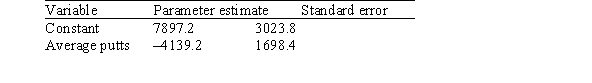
Where the deviations i are assumed to be independent and Normally distributed with a mean of 0 and a standard deviation of .This model was fit to the data using the method of least squares.The following results were obtained from statistical software.
 Suppose the researchers conducting this study wish to estimate the 1993 winnings when the average number of putts per hole is 1.75.The following results were obtained from statistical software.
  If the researchers wish to estimate the mean winnings for all tour pros whose average number of putts per hole is 1.75,what would be a 95% confidence interval for the mean winnings?
A)(77.7,1229.4)
B)(530.6,776.6)
C)653.6 ± 61.62
D)653.6 ± 123.24
Where the deviations i are assumed to be independent and Normally distributed with a mean of 0 and a standard deviation of .This model was fit to the data using the method of least squares.The following results were obtained from statistical software.
Suppose the researchers conducting this study wish to estimate the 1993 winnings when the average number of putts per hole is 1.75.The following results were obtained from statistical software. If the researchers wish to estimate the mean winnings for all tour pros whose average number of putts per hole is 1.75,what would be a 95% confidence interval for the mean winnings?A)(77.7,1229.4)
B)(530.6,776.6)
C)653.6 ± 61.62
D)653.6 ± 123.24
سؤال
Which of the following statements about simple linear regression is/are FALSE?
A)The term "residual" refers to the difference between the observed response and the predicted response using the regression equation.
B)If and
and
 are the intercept and slope,respectively,of the least-squares line,
 is an unbiased estimator of the mean response when
 .
.
C)The estimate of is given by s = .
.
D)The sum to zero.
A)The term "residual" refers to the difference between the observed response and the predicted response using the regression equation.
B)If
and are the intercept and slope,respectively,of the least-squares line, is an unbiased estimator of the mean response when .C)The estimate of is given by s =
.D)The
sum to zero. سؤال
There is an old saying in golf: "You drive for show and you putt for dough." The point is that good putting is more important than long driving for shooting low scores and hence winning money.To see if this is the case,data on the top 69 money winners on the PGA tour in 1993 are examined.The average number of putts per hole for each player is used to predict the total winnings (in thousands of dollars)using the simple linear regression model (1993 winnings)i = 0 + 1(average number of putts per hole)i + i,
Where the deviations i are assumed to be independent and Normally distributed with a mean of 0 and a standard deviation of .This model was fit to the data using the method of least squares.The following results were obtained from statistical software.
 What is the value of the intercept of the least-squares regression line?
A)1698.4
B)3023.8
C)-4139.2
D)7897.2
Where the deviations i are assumed to be independent and Normally distributed with a mean of 0 and a standard deviation of .This model was fit to the data using the method of least squares.The following results were obtained from statistical software.
What is the value of the intercept of the least-squares regression line?A)1698.4
B)3023.8
C)-4139.2
D)7897.2
سؤال
There is an old saying in golf: "You drive for show and you putt for dough." The point is that good putting is more important than long driving for shooting low scores and hence winning money.To see if this is the case,data on the top 69 money winners on the PGA tour in 1993 are examined.The average number of putts per hole for each player is used to predict the total winnings (in thousands of dollars)using the simple linear regression model (1993 winnings)i = 0 + 1(average number of putts per hole)i + i,
Where the deviations i are assumed to be independent and Normally distributed with a mean of 0 and a standard deviation of .This model was fit to the data using the method of least squares.The following results were obtained from statistical software.
 The quantity s = 281.8 is an estimate of the standard deviation of the deviations in the simple linear regression model.What are the degrees of freedom for this estimate?
A)66
B)67
C)68
D)69
Where the deviations i are assumed to be independent and Normally distributed with a mean of 0 and a standard deviation of .This model was fit to the data using the method of least squares.The following results were obtained from statistical software.
The quantity s = 281.8 is an estimate of the standard deviation of the deviations in the simple linear regression model.What are the degrees of freedom for this estimate?A)66
B)67
C)68
D)69
سؤال
The statistical model for simple linear regression has the form  ,i = 1,2,…,n.Which of the following statements about this statistical model is/are TRUE?
A)The are assumed to be Normally distributed with a mean of 0 and a standard deviation of .
B)The parameters of this model are ,
,
 ,and .
C) is the mean response when
  .
.
D)The ,i = 1,2,…,n are independent.
E)All of the above are true.
,i = 1,2,…,n.Which of the following statements about this statistical model is/are TRUE?A)The
are assumed to be Normally distributed with a mean of 0 and a standard deviation of .B)The parameters of this model are
, ,and .C)
is the mean response when .D)The
,i = 1,2,…,n are independent.E)All of the above are true.
سؤال
There is an old saying in golf: "You drive for show and you putt for dough." The point is that good putting is more important than long driving for shooting low scores and hence winning money.To see if this is the case,data on the top 69 money winners on the PGA tour in 1993 are examined.The average number of putts per hole for each player is used to predict the total winnings (in thousands of dollars)using the simple linear regression model (1993 winnings)i = 0 + 1(average number of putts per hole)i + i,
Where the deviations i are assumed to be independent and Normally distributed with a mean of 0 and a standard deviation of .This model was fit to the data using the method of least squares.The following results were obtained from statistical software.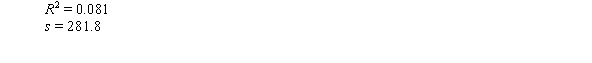
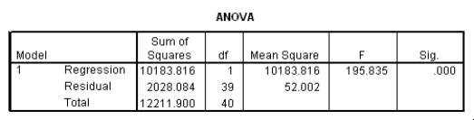
 The following (partial)ANOVA table was obtained from statistical software.
  What is the value of the F statistic for testing the hypotheses H0: 1 = 0 versus Ha: 1 0?
A)0.089
B)2.44
C)4.72
D)5.94
Where the deviations i are assumed to be independent and Normally distributed with a mean of 0 and a standard deviation of .This model was fit to the data using the method of least squares.The following results were obtained from statistical software.
The following (partial)ANOVA table was obtained from statistical software. What is the value of the F statistic for testing the hypotheses H0: 1 = 0 versus Ha: 1 0?A)0.089
B)2.44
C)4.72
D)5.94
سؤال
There is an old saying in golf: "You drive for show and you putt for dough." The point is that good putting is more important than long driving for shooting low scores and hence winning money.To see if this is the case,data on the top 69 money winners on the PGA tour in 1993 are examined.The average number of putts per hole for each player is used to predict the total winnings (in thousands of dollars)using the simple linear regression model (1993 winnings)i = 0 + 1(average number of putts per hole)i + i,
Where the deviations i are assumed to be independent and Normally distributed with a mean of 0 and a standard deviation of .This model was fit to the data using the method of least squares.The following results were obtained from statistical software.
 Suppose the researchers conducting this study wish to test the hypotheses H0: 1 = 0 versus Ha: 1< 0.What is the value of the t statistic for this test?
A)-2.44
B)-1.91
C)2.44
D)2.61
Where the deviations i are assumed to be independent and Normally distributed with a mean of 0 and a standard deviation of .This model was fit to the data using the method of least squares.The following results were obtained from statistical software.
Suppose the researchers conducting this study wish to test the hypotheses H0: 1 = 0 versus Ha: 1< 0.What is the value of the t statistic for this test?A)-2.44
B)-1.91
C)2.44
D)2.61
سؤال
There is an old saying in golf: "You drive for show and you putt for dough." The point is that good putting is more important than long driving for shooting low scores and hence winning money.To see if this is the case,data on the top 69 money winners on the PGA tour in 1993 are examined.The average number of putts per hole for each player is used to predict the total winnings (in thousands of dollars)using the simple linear regression model (1993 winnings)i = 0 + 1(average number of putts per hole)i + i,
Where the deviations i are assumed to be independent and Normally distributed with a mean of 0 and a standard deviation of .This model was fit to the data using the method of least squares.The following results were obtained from statistical software.
 Which of the following conclusions seems most justified?
A)There is no evidence of a relation between the average number of putts per round and the 1993 winnings of PGA tour pros.
B)There is distinct evidence (P-value less than 0.05)that there is a positive correlation between 1993 winnings and average number of putts per round.
C)There is some evidence that PGA tour pros who averaged fewer putts per round had higher winnings in 1993.
D)The presence of strongly influential observations in these data makes it impossible to draw any conclusions about the relationship between 1993 winnings and average number of putts per round.
Where the deviations i are assumed to be independent and Normally distributed with a mean of 0 and a standard deviation of .This model was fit to the data using the method of least squares.The following results were obtained from statistical software.
Which of the following conclusions seems most justified?A)There is no evidence of a relation between the average number of putts per round and the 1993 winnings of PGA tour pros.
B)There is distinct evidence (P-value less than 0.05)that there is a positive correlation between 1993 winnings and average number of putts per round.
C)There is some evidence that PGA tour pros who averaged fewer putts per round had higher winnings in 1993.
D)The presence of strongly influential observations in these data makes it impossible to draw any conclusions about the relationship between 1993 winnings and average number of putts per round.
سؤال
Do heavier cars use more gasoline? To answer this question,a researcher randomly selected 15 cars.He collected their weight (in hundreds of pounds)and the mileage (MPG)for each car.From a scatter plot made with the data,a linear model seemed appropriate.The following output was obtained from SPSS: 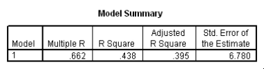
 What is the equation of the least-squares regression line?
A)ŷ = -0.52 x + 0.164
B)ŷ = 40.44 - 0.52x
C)ŷ = 40.44 + 6.28x
D)y = 40.44 + 0.52x
What is the equation of the least-squares regression line?A)ŷ = -0.52 x + 0.164
B)ŷ = 40.44 - 0.52x
C)ŷ = 40.44 + 6.28x
D)y = 40.44 + 0.52x
سؤال
There is an old saying in golf: "You drive for show and you putt for dough." The point is that good putting is more important than long driving for shooting low scores and hence winning money.To see if this is the case,data on the top 69 money winners on the PGA tour in 1993 are examined.The average number of putts per hole for each player is used to predict the total winnings (in thousands of dollars)using the simple linear regression model (1993 winnings)i = 0 + 1(average number of putts per hole)i + i,
Where the deviations i are assumed to be independent and Normally distributed with a mean of 0 and a standard deviation of .This model was fit to the data using the method of least squares.The following results were obtained from statistical software.
 What is an approximate 95% confidence interval for the slope 1?
A)-4139.2 ± 1698.2
B)-4139.2 ± 3396.4
C)7897.2 ± 3023.8
D)7897.2 ± 6047.6
Where the deviations i are assumed to be independent and Normally distributed with a mean of 0 and a standard deviation of .This model was fit to the data using the method of least squares.The following results were obtained from statistical software.
What is an approximate 95% confidence interval for the slope 1?A)-4139.2 ± 1698.2
B)-4139.2 ± 3396.4
C)7897.2 ± 3023.8
D)7897.2 ± 6047.6
سؤال
The data referred to in this question were collected on 41 employees of a large company.The company is trying to predict the current salary of its employees from their starting salary (both expressed in thousands of dollars).The SPSS regression output is given below as well as some summary measures: 


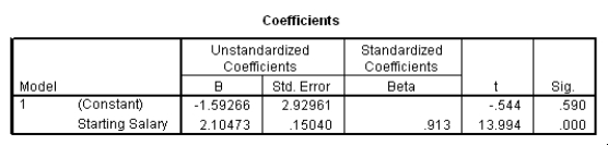 What is the value of the estimate for ,the standard deviation of the model deviations i?
A)0.15
B)2.93
C)7.21
D)52.0
What is the value of the estimate for ,the standard deviation of the model deviations i?A)0.15
B)2.93
C)7.21
D)52.0
سؤال
Do heavier cars use more gasoline? To answer this question,a researcher randomly selected 15 cars.He collected their weight (in hundreds of pounds)and the mileage (MPG)for each car.From a scatter plot made with the data,a linear model seemed appropriate.The following output was obtained from SPSS: 
 To test if there is a significant straight-line relationship between the weight and the mileage of a car,we can perform a t test.What is the value of the t statistic for this test?
A)t = -3.182
B)t = 6.445
C)t = 6.780
D)This cannot be determined from the information given.
To test if there is a significant straight-line relationship between the weight and the mileage of a car,we can perform a t test.What is the value of the t statistic for this test?A)t = -3.182
B)t = 6.445
C)t = 6.780
D)This cannot be determined from the information given.
سؤال
Which of the following statements about the simple linear regression model and its least squares fit is/are FALSE?
A)The ANOVA table gives degrees of freedom,sum of squares,and mean squares for the model,error,and total sources of variation.
B)The ANOVA F statistic is the ratio MSM/MSE.
C)The ANOVA F statistic has an F(1,n - 2)under the null hypothesis H0:
= 0.
D)The ANOVA F statistic is particularly useful because it tests the H0: = 0 against the one-sided alternative Ha:

> 0.
E)The ratio SSM/SST is equal to .
.
A)The ANOVA table gives degrees of freedom,sum of squares,and mean squares for the model,error,and total sources of variation.
B)The ANOVA F statistic is the ratio MSM/MSE.
C)The ANOVA F statistic has an F(1,n - 2)under the null hypothesis H0:
= 0.
D)The ANOVA F statistic is particularly useful because it tests the H0:
= 0 against the one-sided alternative Ha: > 0.
E)The ratio SSM/SST is equal to
. سؤال
There is an old saying in golf: "You drive for show and you putt for dough." The point is that good putting is more important than long driving for shooting low scores and hence winning money.To see if this is the case,data on the top 69 money winners on the PGA tour in 1993 are examined.The average number of putts per hole for each player is used to predict the total winnings (in thousands of dollars)using the simple linear regression model (1993 winnings)i = 0 + 1(average number of putts per hole)i + i,
Where the deviations i are assumed to be independent and Normally distributed with a mean of 0 and a standard deviation of .This model was fit to the data using the method of least squares.The following results were obtained from statistical software.
 Suppose the researchers conducting this study wish to estimate the 1993 winnings when the average number of putts per hole is 1.75.The following results were obtained from statistical software.
 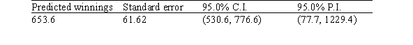 If the researchers wish to estimate the winnings for a particular tour pro whose average number of putts per hole is 1.75,what would be a 95% prediction interval for the winnings?
A)(77.7,1229.4)
B)(530.6,776.6)
C)653.6 ± 61.62
D)653.6 ± 123.24
Where the deviations i are assumed to be independent and Normally distributed with a mean of 0 and a standard deviation of .This model was fit to the data using the method of least squares.The following results were obtained from statistical software.
Suppose the researchers conducting this study wish to estimate the 1993 winnings when the average number of putts per hole is 1.75.The following results were obtained from statistical software. If the researchers wish to estimate the winnings for a particular tour pro whose average number of putts per hole is 1.75,what would be a 95% prediction interval for the winnings?A)(77.7,1229.4)
B)(530.6,776.6)
C)653.6 ± 61.62
D)653.6 ± 123.24
سؤال
There is an old saying in golf: "You drive for show and you putt for dough." The point is that good putting is more important than long driving for shooting low scores and hence winning money.To see if this is the case,data on the top 69 money winners on the PGA tour in 1993 are examined.The average number of putts per hole for each player is used to predict the total winnings (in thousands of dollars)using the simple linear regression model (1993 winnings)i = 0 + 1(average number of putts per hole)i + i,
Where the deviations i are assumed to be independent and Normally distributed with a mean of 0 and a standard deviation of .This model was fit to the data using the method of least squares.The following results were obtained from statistical software.
 The following (partial)ANOVA table was obtained from statistical software.
 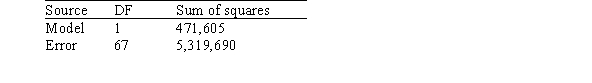 What is the value of the SST,the total sum of squares?
A)79,398
B)471,605
C)5,319,690
D)5,791,295
Where the deviations i are assumed to be independent and Normally distributed with a mean of 0 and a standard deviation of .This model was fit to the data using the method of least squares.The following results were obtained from statistical software.
The following (partial)ANOVA table was obtained from statistical software. What is the value of the SST,the total sum of squares?A)79,398
B)471,605
C)5,319,690
D)5,791,295
سؤال
Do heavier cars use more gasoline? To answer this question,a researcher randomly selected 15 cars.He collected their weight (in hundreds of pounds)and the mileage (MPG)for each car.From a scatter plot made with the data,a linear model seemed appropriate.The following output was obtained from SPSS: 
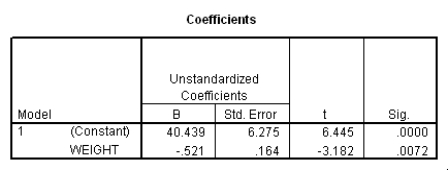 Which of the following descriptions of the value of the slope is the correct description?
A)We cannot interpret the slope because we cannot have a negative weight of a car.
B)We estimate the mileage to decrease by 0.521 miles per gallon when the weight of a car increases by 1 pound.
C)We estimate the mileage to decrease by 0.521 miles per gallon when the weight of a car increases by 100 pounds.
D)We estimate the mileage to decrease by 52.1 miles per gallon when the weight of a car increases by 100 pounds.
Which of the following descriptions of the value of the slope is the correct description?A)We cannot interpret the slope because we cannot have a negative weight of a car.
B)We estimate the mileage to decrease by 0.521 miles per gallon when the weight of a car increases by 1 pound.
C)We estimate the mileage to decrease by 0.521 miles per gallon when the weight of a car increases by 100 pounds.
D)We estimate the mileage to decrease by 52.1 miles per gallon when the weight of a car increases by 100 pounds.
سؤال
The data referred to in this question were collected on 41 employees of a large company.The company is trying to predict the current salary of its employees from their starting salary (both expressed in thousands of dollars).The SPPS regression output is given below as well as some summary measures: 


 What is an approximate 95% confidence interval for the slope 1?
A)(-7.57,4.39)
B)(-4.52,1.34)
C)(1.80,2.41)
D)(1.95,2.26)
What is an approximate 95% confidence interval for the slope 1?A)(-7.57,4.39)
B)(-4.52,1.34)
C)(1.80,2.41)
D)(1.95,2.26)
سؤال
The data referred to in this question were collected on 41 employees of a large company.The company is trying to predict the current salary of its employees from their starting salary (both expressed in thousands of dollars).The SPPS regression output is given below as well as some summary measures: 


 Suppose we wish to test the hypotheses H0: 1 = 2 versus Ha: 1 2.Together with an insignificant constant in this model,this would imply that the employees currently earn about twice as much as their starting salary.At the 5% significance level,would we reject the null hypothesis?
A)Yes
B)No
C)This cannot be determined from the information given.
Suppose we wish to test the hypotheses H0: 1 = 2 versus Ha: 1 2.Together with an insignificant constant in this model,this would imply that the employees currently earn about twice as much as their starting salary.At the 5% significance level,would we reject the null hypothesis?A)Yes
B)No
C)This cannot be determined from the information given.
سؤال
The data referred to in this question were collected on 41 employees of a large company.The company is trying to predict the current salary of its employees from their starting salary (both expressed in thousands of dollars).The SPSS regression output is given below as well as some summary measures: 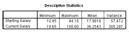

 How would a 90% confidence interval for the average current salary for all employees who started with a salary of $15,300 compare to a 90% confidence interval for the current salary of an individual with a starting salary of $15,300?
A)It would be narrower.
B)It would be the same.
C)It would be wider.
D)This cannot be determined from the information given.
How would a 90% confidence interval for the average current salary for all employees who started with a salary of $15,300 compare to a 90% confidence interval for the current salary of an individual with a starting salary of $15,300?A)It would be narrower.
B)It would be the same.
C)It would be wider.
D)This cannot be determined from the information given.
سؤال
The data referred to in this question were collected on 41 employees of a large company.The company is trying to predict the current salary of its employees from their starting salary (both expressed in thousands of dollars).The SPSS regression output is given below as well as some summary measures: 


 John Doe works for this company.He started with a salary of $15,300.Predict his current salary with a 90% confidence interval.Express the interval in the appropriate units.
A)($15,683;$45,537)
B)($18,204;$43,015)
C)($28,580;$32,640)
D)($31,516;$32,885)
John Doe works for this company.He started with a salary of $15,300.Predict his current salary with a 90% confidence interval.Express the interval in the appropriate units.A)($15,683;$45,537)
B)($18,204;$43,015)
C)($28,580;$32,640)
D)($31,516;$32,885)
سؤال
The statistical model for simple linear regression is written as  ,where
  represents the mean of a Normally distributed response variable and x represents the explanatory variable.The parameters
  and
and  are estimated,giving the linear regression model defined by
  ,with standard deviation = 5. What is the y-intercept for the regression line?
A)10
B)70
C)80
D)60
,where represents the mean of a Normally distributed response variable and x represents the explanatory variable.The parameters and are estimated,giving the linear regression model defined by ,with standard deviation = 5. What is the y-intercept for the regression line?A)10
B)70
C)80
D)60
سؤال
A random sample of 79 companies from the Forbes 500 list (which actually consists of nearly 800 companies)was selected,and the relationship between sales (in hundreds of thousands of dollars)and profits (in hundreds of thousands of dollars)was investigated by regression.The following results were obtained from statistical software. 
 The following (partial)ANOVA table was obtained from statistical software.
  What is the value of the SST,the total sum of squares?
A)16,074,978
B)16,734,234
C)32,809,212
D)49,543,448
The following (partial)ANOVA table was obtained from statistical software. What is the value of the SST,the total sum of squares?A)16,074,978
B)16,734,234
C)32,809,212
D)49,543,448
سؤال
A random sample of 79 companies from the Forbes 500 list (which actually consists of nearly 800 companies)was selected,and the relationship between sales (in hundreds of thousands of dollars)and profits (in hundreds of thousands of dollars)was investigated by regression.The following results were obtained from statistical software. 
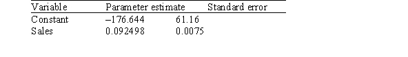 What is approximately the value of the intercept of the least-squares regression line?
A)0.0075
B)0.0925
C)61.16
D)-176.64
What is approximately the value of the intercept of the least-squares regression line?A)0.0075
B)0.0925
C)61.16
D)-176.64
سؤال
As in most professional sports,statistics are collected in the National Hockey League.In the 2006-2007 season,teams played 82 games.A team was awarded 2 points for a win and 1 point if the game was tied at the end of regulation time but then lost in overtime.For each of the 30 teams,data on the number of goals scored per game (Goals/G)and the percentage of the 164 possible points they won (Win%)during the season were collected.The following graph shows the plotted points for the variables Win% and Goals/G and the simple linear regression line fitted using least squares.  From the computer output for the least-squares fit,the estimated equation was found to be
  ,
,  = 0.398,and
  = 60.29.Also,it was determined from the output that
  = 12.800 and
  = 4.418. Which of the following statements is/are FALSE?
A)An amount of 39.8% of the variation in the winning percent variable is explained by the least-squares regression on the number of goals scored per game.
B)An increase of 1 goal per game results in an increase of about 19% in winning percent.
C)If a team scores 3 goals per game,we would predict the team would have a Win% of 55%.
D)The Ottawa Senators scored 3.49 goals per game and their Win% was 64.0.The residual for Ottawa was then -3.32.
E)The mean value of the Win% variable is 0.932 when the Goals/G is 0.
From the computer output for the least-squares fit,the estimated equation was found to be , = 0.398,and = 60.29.Also,it was determined from the output that = 12.800 and = 4.418. Which of the following statements is/are FALSE?A)An amount of 39.8% of the variation in the winning percent variable is explained by the least-squares regression on the number of goals scored per game.
B)An increase of 1 goal per game results in an increase of about 19% in winning percent.
C)If a team scores 3 goals per game,we would predict the team would have a Win% of 55%.
D)The Ottawa Senators scored 3.49 goals per game and their Win% was 64.0.The residual for Ottawa was then -3.32.
E)The mean value of the Win% variable is 0.932 when the Goals/G is 0.
سؤال
A random sample of 79 companies from the Forbes 500 list (which actually consists of nearly 800 companies)was selected,and the relationship between sales (in hundreds of thousands of dollars)and profits (in hundreds of thousands of dollars)was investigated by regression.The following results were obtained from statistical software. 
 Suppose the researchers conducting the study wish to test the hypotheses H0: 1 = 0 versus Ha: 1> 0.What do we know about the P-value of this test?
A)The P-value is greater than 0.10.
B)The P-value is between 0.05 and 0.10.
C)The P-value is between 0.01 and 0.05.
D)The P-value is less than 0.01.
Suppose the researchers conducting the study wish to test the hypotheses H0: 1 = 0 versus Ha: 1> 0.What do we know about the P-value of this test?A)The P-value is greater than 0.10.
B)The P-value is between 0.05 and 0.10.
C)The P-value is between 0.01 and 0.05.
D)The P-value is less than 0.01.
سؤال
A random sample of 79 companies from the Forbes 500 list (which actually consists of nearly 800 companies)was selected,and the relationship between sales (in hundreds of thousands of dollars)and profits (in hundreds of thousands of dollars)was investigated by regression.The following results were obtained from statistical software. 
 The following (partial)ANOVA table was obtained from statistical software.
  What is the value of the F statistic for testing the hypotheses H0: 1 = 0 versus Ha: 1 0?
A)1.96
B)77
C)150.97
D)217,328
The following (partial)ANOVA table was obtained from statistical software. What is the value of the F statistic for testing the hypotheses H0: 1 = 0 versus Ha: 1 0?A)1.96
B)77
C)150.97
D)217,328
سؤال
A random sample of 79 companies from the Forbes 500 list (which actually consists of nearly 800 companies)was selected,and the relationship between sales (in hundreds of thousands of dollars)and profits (in hundreds of thousands of dollars)was investigated by regression.The following results were obtained from statistical software. 
 What is an approximate 90% confidence interval for the slope 1?
A)-0.09 ± 0.0075
B)-0.09 ± 0.0125
C)0.09 ± 0.0075
D)0.09 ± 0.0125
What is an approximate 90% confidence interval for the slope 1?A)-0.09 ± 0.0075
B)-0.09 ± 0.0125
C)0.09 ± 0.0075
D)0.09 ± 0.0125
سؤال
The statistical model for simple linear regression is written as  ,where
  represents the mean of a Normally distributed response variable and x represents the explanatory variable.The parameters
  and
and  are estimated,giving the linear regression model defined by
  ,with standard deviation = 5. What is the slope of the regression line?
A)10
B)70
C)80
D)60
,where represents the mean of a Normally distributed response variable and x represents the explanatory variable.The parameters and are estimated,giving the linear regression model defined by ,with standard deviation = 5. What is the slope of the regression line?A)10
B)70
C)80
D)60
سؤال
A random sample of 79 companies from the Forbes 500 list (which actually consists of nearly 800 companies)was selected,and the relationship between sales (in hundreds of thousands of dollars)and profits (in hundreds of thousands of dollars)was investigated by regression.The following results were obtained from statistical software. 
 The following (partial)ANOVA table was obtained from statistical software.
 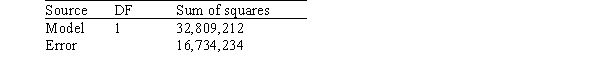 What are the degrees of freedom for SSE,the error sum of squares?
A)2
B)77
C)78
D)79
The following (partial)ANOVA table was obtained from statistical software. What are the degrees of freedom for SSE,the error sum of squares?A)2
B)77
C)78
D)79
سؤال
As in most professional sports,statistics are collected in the National Hockey League.In the 2006-2007 season,teams played 82 games.A team was awarded 2 points for a win and 1 point if the game was tied at the end of regulation time but then lost in overtime.For each of the 30 teams,data on the number of goals scored per game (Goals/G)and the percentage of the 164 possible points they won (Win%)during the season were collected.The following graph shows the plotted points for the variables Win% and Goals/G and the simple linear regression line fitted using least squares.  From the computer output for the least-squares fit,the estimated equation was found to be
  ,
,  = 0.398,and
  = 60.29.Also,it was determined from the output that
  = 12.800 and
  = 4.418. If a test of hypothesis were conducted of H0:
  = 0 against Ha:
  0,what would be the value of the test statistic?
A)t = 0.07
B)z = 0.07
C)z = 4.31
D)F = 4.31
E)t = 4.31
From the computer output for the least-squares fit,the estimated equation was found to be , = 0.398,and = 60.29.Also,it was determined from the output that = 12.800 and = 4.418. If a test of hypothesis were conducted of H0: = 0 against Ha: 0,what would be the value of the test statistic?A)t = 0.07
B)z = 0.07
C)z = 4.31
D)F = 4.31
E)t = 4.31
سؤال
Do heavier cars use more gasoline? To answer this question,a researcher randomly selected 15 cars.He collected their weight (in hundreds of pounds)and the mileage (MPG)for each car.From a scatter plot made with the data,a linear model seemed appropriate.The following output was obtained from SPSS: 
 What is a 95% confidence interval for the slope 1?
A)(-0.875,-0.167)
B)(-0.685,-0.357)
C)(-1.04,0.001)
D)(26.89,53.99)
What is a 95% confidence interval for the slope 1?A)(-0.875,-0.167)
B)(-0.685,-0.357)
C)(-1.04,0.001)
D)(26.89,53.99)
سؤال
A random sample of 79 companies from the Forbes 500 list (which actually consists of nearly 800 companies)was selected,and the relationship between sales (in hundreds of thousands of dollars)and profits (in hundreds of thousands of dollars)was investigated by regression.The following results were obtained from statistical software. 
 Suppose the researchers conducting this study wish to estimate the profits (in hundreds of thousands of dollars)for companies that had sales (in hundreds of thousands of dollars)of 500.The following results were obtained from statistical software.
 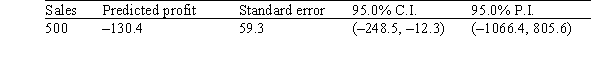 If the researchers wish to estimate the profits for a particular company that had sales of 500,what would be a 95% prediction interval for the profits?
A)(-1066.4,805.6)
B)(-248.5,-12.3)
C)-130.4 ± 59.3
D)500 ± 59.3
Suppose the researchers conducting this study wish to estimate the profits (in hundreds of thousands of dollars)for companies that had sales (in hundreds of thousands of dollars)of 500.The following results were obtained from statistical software. If the researchers wish to estimate the profits for a particular company that had sales of 500,what would be a 95% prediction interval for the profits?A)(-1066.4,805.6)
B)(-248.5,-12.3)
C)-130.4 ± 59.3
D)500 ± 59.3
سؤال
As in most professional sports,statistics are collected in the National Hockey League.In the 2006-2007 season,teams played 82 games.A team was awarded 2 points for a win and 1 point if the game was tied at the end of regulation time but then lost in overtime.For each of the 30 teams,data on the number of goals scored per game (Goals/G)and the percentage of the 164 possible points they won (Win%)during the season were collected.The following graph shows the plotted points for the variables Win% and Goals/G and the simple linear regression line fitted using least squares.  From the computer output for the least-squares fit,the estimated equation was found to be
 = 0.398,and
  = 60.29.Also,it was determined from the output that
  = 12.800 and
  = 4.418.For the 2006-2007 season,teams scored an average of
  = 2.88 goals per game.For the population of teams that score 2.5 goals per game,the standard error of the estimated mean Win% is
  = 2.197.What is the estimated mean Win% for the population of teams that score 2.5 goals per game?
A)42.7%
B)53.6%
C)48.5%
D)55.7%
E)Not within ± 2% of any of the above
From the computer output for the least-squares fit,the estimated equation was found to be = 0.398,and = 60.29.Also,it was determined from the output that = 12.800 and = 4.418.For the 2006-2007 season,teams scored an average of = 2.88 goals per game.For the population of teams that score 2.5 goals per game,the standard error of the estimated mean Win% is = 2.197.What is the estimated mean Win% for the population of teams that score 2.5 goals per game?A)42.7%
B)53.6%
C)48.5%
D)55.7%
E)Not within ± 2% of any of the above
سؤال
A random sample of 79 companies from the Forbes 500 list (which actually consists of nearly 800 companies)was selected,and the relationship between sales (in hundreds of thousands of dollars)and profits (in hundreds of thousands of dollars)was investigated by regression.The following results were obtained from statistical software. 
 Suppose the researchers conducting this study wish to estimate the profits (in hundreds of thousands of dollars)for companies that had sales (in hundreds of thousands of dollars)of 500.The following results were obtained from statistical software.
  If the researchers wish to estimate the mean profits for all companies that had sales of 500,what would be a 95% confidence interval for the mean profits?
A)(-1066.4,805.6)
B)(-248.5,-12.3)
C)-130.4 ± 59.3
D)500 ± 59.3
Suppose the researchers conducting this study wish to estimate the profits (in hundreds of thousands of dollars)for companies that had sales (in hundreds of thousands of dollars)of 500.The following results were obtained from statistical software. If the researchers wish to estimate the mean profits for all companies that had sales of 500,what would be a 95% confidence interval for the mean profits?A)(-1066.4,805.6)
B)(-248.5,-12.3)
C)-130.4 ± 59.3
D)500 ± 59.3
سؤال
A random sample of 79 companies from the Forbes 500 list (which actually consists of nearly 800 companies)was selected,and the relationship between sales (in hundreds of thousands of dollars)and profits (in hundreds of thousands of dollars)was investigated by regression.The following results were obtained from statistical software. 
 Is there strong evidence of a straight-line relationship between sales and profits? Explain briefly.
A)Yes,because the slope of the least-squares line is positive
B)Yes,because the P-value for testing if the slope is zero is quite small
C)No,because the value of the square of the correlation is relatively small
D)It is impossible to say because we are not given the actual value of the correlation.
Is there strong evidence of a straight-line relationship between sales and profits? Explain briefly.A)Yes,because the slope of the least-squares line is positive
B)Yes,because the P-value for testing if the slope is zero is quite small
C)No,because the value of the square of the correlation is relatively small
D)It is impossible to say because we are not given the actual value of the correlation.
سؤال
The statistical model for simple linear regression is written as  ,where
  represents the mean of a Normally distributed response variable and x represents the explanatory variable.The parameters
  and
and  are estimated,giving the linear regression model defined by
  ,with standard deviation = 5. The explanatory variable x is ________.
A)quantitative
B)qualitative
C)categorical
D)None of the above
,where represents the mean of a Normally distributed response variable and x represents the explanatory variable.The parameters and are estimated,giving the linear regression model defined by ,with standard deviation = 5. The explanatory variable x is ________.A)quantitative
B)qualitative
C)categorical
D)None of the above
سؤال
As in most professional sports,statistics are collected in the National Hockey League.In the 2006-2007 season,teams played 82 games.A team was awarded 2 points for a win and 1 point if the game was tied at the end of regulation time but then lost in overtime.For each of the 30 teams,data on the number of goals scored per game (Goals/G)and the percentage of the 164 possible points they won (Win%)during the season were collected.The following graph shows the plotted points for the variables Win% and Goals/G and the simple linear regression line fitted using least squares.  From the computer output for the least-squares fit,the estimated equation was found to be
  ,
,  = 0.398,and
  = 60.29.Also,it was determined from the output that
  = 12.800 and
  = 4.418.We are told that
  = 60.29.How many degrees of freedom are associated with this statistic?
A)29
B)1
C)30
D)28
E)None of the above
From the computer output for the least-squares fit,the estimated equation was found to be , = 0.398,and = 60.29.Also,it was determined from the output that = 12.800 and = 4.418.We are told that = 60.29.How many degrees of freedom are associated with this statistic?A)29
B)1
C)30
D)28
E)None of the above
سؤال
As in most professional sports,statistics are collected in the National Hockey League.In the 2006-2007 season,teams played 82 games.A team was awarded 2 points for a win and 1 point if the game was tied at the end of regulation time but then lost in overtime.For each of the 30 teams,data on the number of goals scored per game (Goals/G)and the percentage of the 164 possible points they won (Win%)during the season were collected.The following graph shows the plotted points for the variables Win% and Goals/G and the simple linear regression line fitted using least squares. 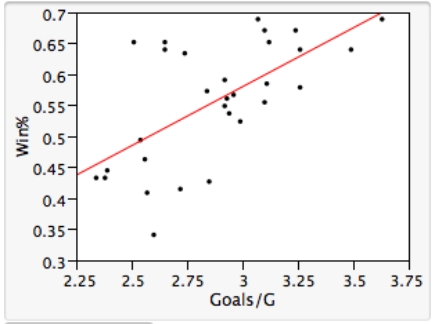 From the computer output for the least-squares fit,the estimated equation was found to be
  ,
,  = 0.398,and
  = 60.29.Also,it was determined from the output that
  = 12.800 and
  = 4.418. A plot of the residuals from the least-squares fit against the Goals/G variable is shown below.
 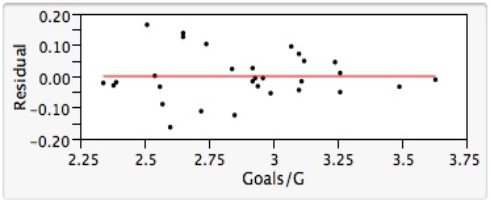 What statements about residuals and/or about this residual plot is/are FALSE?
A)There does not appear to be any particular pattern to the residuals on the plot.
B)The residual plot shows that the residuals do approximately follow a Normal distribution,as the statistical model requires.
C)Residuals from a least-squares fit in simple linear regression always sum to zero.
D)None of the residuals look as though they would be considered to be outliers.
E)The residuals appear to vary randomly about their mean of zero.
From the computer output for the least-squares fit,the estimated equation was found to be , = 0.398,and = 60.29.Also,it was determined from the output that = 12.800 and = 4.418. A plot of the residuals from the least-squares fit against the Goals/G variable is shown below. What statements about residuals and/or about this residual plot is/are FALSE?A)There does not appear to be any particular pattern to the residuals on the plot.
B)The residual plot shows that the residuals do approximately follow a Normal distribution,as the statistical model requires.
C)Residuals from a least-squares fit in simple linear regression always sum to zero.
D)None of the residuals look as though they would be considered to be outliers.
E)The residuals appear to vary randomly about their mean of zero.
سؤال
As in most professional sports,statistics are collected in the National Hockey League.In the 2006-2007 season,teams played 82 games.A team was awarded 2 points for a win and 1 point if the game was tied at the end of regulation time but then lost in overtime.For each of the 30 teams,data on the number of goals scored per game (Goals/G)and the percentage of the 164 possible points they won (Win%)during the season were collected.The following graph shows the plotted points for the variables Win% and Goals/G and the simple linear regression line fitted using least squares.  From the computer output for the least-squares fit,the estimated equation was found to be
  ,
,  = 0.398,and
  = 60.29.Also,it was determined from the output that
  = 12.800 and
  = 4.418.What would the approximate 96% confidence interval be for the true slope
  ?
?
A)19.022 ± 2.054(12.800)
B)19.022 ± 2.154(4.418)
C)0.932 ± 2.154(12.800)
D)19.022 ± 2.054(4.418)
E)0.932 ± 2.154 (12.800)
From the computer output for the least-squares fit,the estimated equation was found to be , = 0.398,and = 60.29.Also,it was determined from the output that = 12.800 and = 4.418.What would the approximate 96% confidence interval be for the true slope ?A)19.022 ± 2.054(12.800)
B)19.022 ± 2.154(4.418)
C)0.932 ± 2.154(12.800)
D)19.022 ± 2.054(4.418)
E)0.932 ± 2.154 (12.800)
سؤال
سؤال
The statistical model for simple linear regression is written as  ,where
  represents the mean of a Normally distributed response variable and x represents the explanatory variable.The parameters
  and
and  are estimated,giving the linear regression model defined by
  ,with standard deviation = 5. What is the distribution of the test statistic used to test the null hypothesis
  against the alternative hypothesis
  ? (Note: Assume n is the sample size. )
A)N(0,1)
B)N(0,2)
C)t(n - 1)
D)t(n - 2)
,where represents the mean of a Normally distributed response variable and x represents the explanatory variable.The parameters and are estimated,giving the linear regression model defined by ,with standard deviation = 5. What is the distribution of the test statistic used to test the null hypothesis against the alternative hypothesis ? (Note: Assume n is the sample size. )A)N(0,1)
B)N(0,2)
C)t(n - 1)
D)t(n - 2)
سؤال
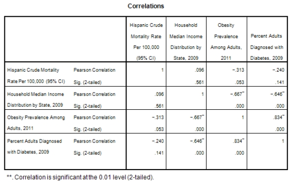
A recent study was done to assess factors that put Hispanic populations more at risk for obesity and related chronic diseases,such as diabetes and heart disease,than non-Hispanic populations.Data were collected on several factors,such as the crude morality rate of Hispanics,obesity prevalence,percent of adults diagnosed with diabetes,and median income at the state level.Pearson's Correlations were used to examine the strength of the relationship between obesity and the other variables,as a way of observing which characteristics were associated with high prevalence of obesity.In addition,a simple linear regression was used to model the relationship between diabetes and obesity.The results from SPSS are shown below. 


 What is the value of the F statistic to test the null hypothesis that
  versus the alternative hypothesis that
  ?
?
A)111.64
B)10.16
C).83
D)None of the above
What is the value of the F statistic to test the null hypothesis that versus the alternative hypothesis that ?A)111.64
B)10.16
C).83
D)None of the above
سؤال
The statistical model for simple linear regression is written as  ,where
  represents the mean of a Normally distributed response variable and x represents the explanatory variable.The parameters
  and
and  are estimated,giving the linear regression model defined by
  ,with standard deviation = 5. What is the range of values for 68% of the observed responses when x = 20 using the 68-95-99.7 rule?
A)265 to 275
B)270 to 275
C)265 to 270
D)None of the above
,where represents the mean of a Normally distributed response variable and x represents the explanatory variable.The parameters and are estimated,giving the linear regression model defined by ,with standard deviation = 5. What is the range of values for 68% of the observed responses when x = 20 using the 68-95-99.7 rule?A)265 to 275
B)270 to 275
C)265 to 270
D)None of the above
سؤال
Suppose we are given the following information: Sample size,n,= 100
Standard error of slope of the regression line, = 2
= 2  = 100 + 4x
What is the predicted value of the response when x = 5?
A)120
B)100
C)20
D)None of the above
Standard error of slope of the regression line,
= 2 = 100 + 4xWhat is the predicted value of the response when x = 5?
A)120
B)100
C)20
D)None of the above
سؤال
A recent study was done to assess factors that put Hispanic populations more at risk for obesity and related chronic diseases,such as diabetes and heart disease,than non-Hispanic populations.Data were collected on several factors,such as the crude morality rate of Hispanics,obesity prevalence,percent of adults diagnosed with diabetes,and median income at the state level.Pearson's Correlations were used to examine the strength of the relationship between obesity and the other variables,as a way of observing which characteristics were associated with high prevalence of obesity.In addition,a simple linear regression was used to model the relationship between diabetes and obesity.The results from SPSS are shown below. 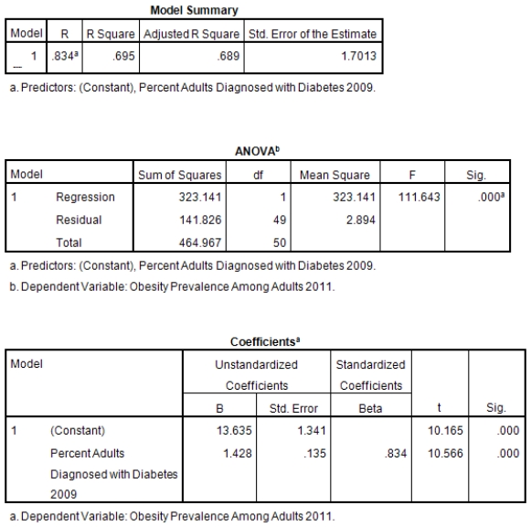


 What is the slope of the least-squares regression line to predict obesity rates from diabetes rates?
A)1.43
B)13.64
C)0
D)None of the above
What is the slope of the least-squares regression line to predict obesity rates from diabetes rates?A)1.43
B)13.64
C)0
D)None of the above
سؤال
The statistical model for simple linear regression is written as  ,where
  represents the mean of a Normally distributed response variable and x represents the explanatory variable.The parameters
  and
and  are estimated,giving the linear regression model defined by
  ,with standard deviation = 5. What is the subpopulation mean when x = 20?
A)270
B)100
C)70
D)None of the above
,where represents the mean of a Normally distributed response variable and x represents the explanatory variable.The parameters and are estimated,giving the linear regression model defined by ,with standard deviation = 5. What is the subpopulation mean when x = 20?A)270
B)100
C)70
D)None of the above
سؤال
A recent study was done to assess factors that put Hispanic populations more at risk for obesity and related chronic diseases,such as diabetes and heart disease,than non-Hispanic populations.Data were collected on several factors,such as the crude morality rate of Hispanics,obesity prevalence,percent of adults diagnosed with diabetes,and median income at the state level.Pearson's Correlations were used to examine the strength of the relationship between obesity and the other variables,as a way of observing which characteristics were associated with high prevalence of obesity.In addition,a simple linear regression was used to model the relationship between diabetes and obesity.The results from SPSS are shown below. 


 What is the sample correlation between obesity prevalence and percent adults diagnosed with diabetes?
A)-.240
B).141
C)1
D)None of the above
What is the sample correlation between obesity prevalence and percent adults diagnosed with diabetes?A)-.240
B).141
C)1
D)None of the above
سؤال
Suppose we are given the following information: Sample size,n,= 100
Standard error of slope of the regression line, = 2
= 2  = 100 + 4x
What is the P-value for a test of the null hypothesis that the slope is zero versus the alternative hypothesis that the slope is not zero?
A).04
B).05
C).02
D)None of the above
Standard error of slope of the regression line,
= 2 = 100 + 4xWhat is the P-value for a test of the null hypothesis that the slope is zero versus the alternative hypothesis that the slope is not zero?
A).04
B).05
C).02
D)None of the above
سؤال
Suppose we are given the following information: Sample size,n,= 100
Standard error of slope of the regression line, = 2
= 2  = 100 + 4x
Is there a statistically significant linear relationship between the response and explanatory variable when the significance level, ,is .01?
A)Yes
B)No
Standard error of slope of the regression line,
= 2 = 100 + 4xIs there a statistically significant linear relationship between the response and explanatory variable when the significance level, ,is .01?
A)Yes
B)No
سؤال
سؤال
Suppose we are given the following information: Sample size,n,= 100
Standard error of slope of the regression line, = 2
= 2  = 100 + 4x
What is the critical value,t*,that is used to compute an 80% confidence interval for 1? (Note: Use software to compute the exact value. )
A).84
B)1.29
C)1.98
D)None of the above
Standard error of slope of the regression line,
= 2 = 100 + 4xWhat is the critical value,t*,that is used to compute an 80% confidence interval for 1? (Note: Use software to compute the exact value. )
A).84
B)1.29
C)1.98
D)None of the above
سؤال
Suppose we are given the following information: Sample size,n,= 100
Standard error of slope of the regression line, = 2
= 2  = 100 + 4x
What is an 80% confidence interval for 1?
A)(-0.71,3.29)
B)(.71,3.29)
C)(-2.71,5.29)
D)None of the above
Standard error of slope of the regression line,
= 2 = 100 + 4xWhat is an 80% confidence interval for 1?
A)(-0.71,3.29)
B)(.71,3.29)
C)(-2.71,5.29)
D)None of the above
سؤال
سؤال
A recent study was done to assess factors that put Hispanic populations more at risk for obesity and related chronic diseases,such as diabetes and heart disease,than non-Hispanic populations.Data were collected on several factors,such as the crude morality rate of Hispanics,obesity prevalence,percent of adults diagnosed with diabetes,and median income at the state level.Pearson's Correlations were used to examine the strength of the relationship between obesity and the other variables,as a way of observing which characteristics were associated with high prevalence of obesity.In addition,a simple linear regression was used to model the relationship between diabetes and obesity.The results from SPSS are shown below. 


 What is the P-value to test that the population correlation is zero verses the alternative that the population correlation is greater than zero?
A)0
B)1
C)It cannot be determined from the given information.
D)None of the above
What is the P-value to test that the population correlation is zero verses the alternative that the population correlation is greater than zero?A)0
B)1
C)It cannot be determined from the given information.
D)None of the above
سؤال
Suppose we are given the following information: Sample size,n,= 100
Standard error of slope of the regression line, = 2
= 2  = 100 + 4x
Would a 95% confidence interval for 1 be larger,smaller,or the same as an 80% confidence interval for 1?
A)Larger
B)Smaller
C)Same
D)It cannot be determined from the information given.
Standard error of slope of the regression line,
= 2 = 100 + 4xWould a 95% confidence interval for 1 be larger,smaller,or the same as an 80% confidence interval for 1?
A)Larger
B)Smaller
C)Same
D)It cannot be determined from the information given.
سؤال
Suppose we are given the following information: Sample size,n,= 100
Standard error of slope of the regression line, = 2
= 2  = 100 + 4x
Suppose an observed response value is 150 when x = 5.What is the value of the residual?
A)150
B)30
C)-30
D)None of the above
Standard error of slope of the regression line,
= 2 = 100 + 4xSuppose an observed response value is 150 when x = 5.What is the value of the residual?
A)150
B)30
C)-30
D)None of the above
سؤال
Suppose we are given the following information: Sample size,n,= 100
Standard error of slope of the regression line, = 2
= 2  = 100 + 4x
What is the test statistic to test the null hypothesis that the slope is zero versus the alternative hypothesis that the slope is not zero?
A)100
B)4
C)2
D)None of the above
Standard error of slope of the regression line,
= 2 = 100 + 4xWhat is the test statistic to test the null hypothesis that the slope is zero versus the alternative hypothesis that the slope is not zero?
A)100
B)4
C)2
D)None of the above
سؤال
سؤال
A recent study was done to assess factors that put Hispanic populations more at risk for obesity and related chronic diseases,such as diabetes and heart disease,than non-Hispanic populations.Data were collected on several factors,such as the crude morality rate of Hispanics,obesity prevalence,percent of adults diagnosed with diabetes,and median income at the state level.Pearson's Correlations were used to examine the strength of the relationship between obesity and the other variables,as a way of observing which characteristics were associated with high prevalence of obesity.In addition,a simple linear regression was used to model the relationship between diabetes and obesity.The results from SPSS are shown below. 


 What is the sample size?
A)100
B)50
C)It cannot be determined from the information given.
D)None of the above
What is the sample size?A)100
B)50
C)It cannot be determined from the information given.
D)None of the above
سؤال
A recent study was done to assess factors that put Hispanic populations more at risk for obesity and related chronic diseases,such as diabetes and heart disease,than non-Hispanic populations.Data were collected on several factors,such as the crude morality rate of Hispanics,obesity prevalence,percent of adults diagnosed with diabetes,and median income at the state level.Pearson's Correlations were used to examine the strength of the relationship between obesity and the other variables,as a way of observing which characteristics were associated with high prevalence of obesity.In addition,a simple linear regression was used to model the relationship between diabetes and obesity.The results from SPSS are shown below. 

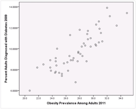
 Is simple linear regression an appropriate statistical procedure to use on these data to study the relationship between obesity and diabetes?
A)Yes,the scatter plot shows a linear relationship between obesity and diabetes.
B)Yes,the scatter plot shows a nonlinear relationship between obesity and diabetes.
C)No,the relationship between obesity and diabetes is not strong enough.
D)No,the data should show a nonlinear pattern.
Is simple linear regression an appropriate statistical procedure to use on these data to study the relationship between obesity and diabetes?A)Yes,the scatter plot shows a linear relationship between obesity and diabetes.
B)Yes,the scatter plot shows a nonlinear relationship between obesity and diabetes.
C)No,the relationship between obesity and diabetes is not strong enough.
D)No,the data should show a nonlinear pattern.
سؤال
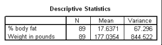
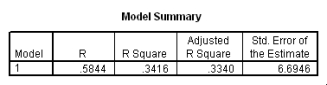
The following scatter plot and SPSS output represent data collected on 89 middle-aged people.The relationship between body weight and percent body fat is to be studied. 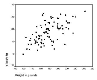


 What is the value of the estimate for ,the standard deviation of the deviations i?
What is the value of the estimate for ,the standard deviation of the deviations i? سؤال
The following scatter plot and SPSS output represent data collected on 89 middle-aged people.The relationship between body weight and percent body fat is to be studied. 


 What is the equation of the least-squares regression line?
What is the equation of the least-squares regression line? سؤال
A study was conducted to monitor the emissions of a noxious substance from a chemical plant and the concentration of the chemical at a location in close proximity to the plant at various times throughout the year.A total of 14 measurements were made.Computer output for the simple linear regression least-squares fit is provided.(Some entries have been omitted and replaced with **. )  What is the estimate of
  ?
?
A)1.514
B)1.143
C)0.794
D)2.292
E)27.506
What is the estimate of ?A)1.514
B)1.143
C)0.794
D)2.292
E)27.506
سؤال
The following scatter plot and SPSS output represent data collected on 89 middle-aged people.The relationship between body weight and percent body fat is to be studied. 


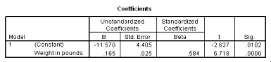 Let be the population correlation between body fat and body weight.What is the value of the t statistic for testing the hypotheses H0: = 0 versus Ha: 0?
Let be the population correlation between body fat and body weight.What is the value of the t statistic for testing the hypotheses H0: = 0 versus Ha: 0? سؤال
In the National Football League (NFL),having an effective passing game is seen to be important in order to win games.The following information for the 32 NFL teams in the 2007 season concerns the points a team scores per game (Pts/Gm)and the percent of its passes that were completed (Pass%).The ANOVA table is provided for the simple linear regression fit of Pts/Gm on Pass%.(Some entries have been omitted and replaced with **). 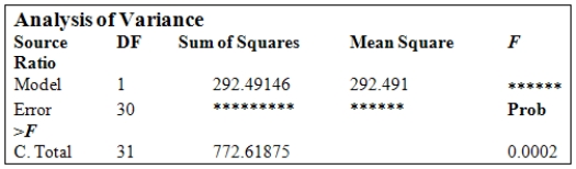 From the computer output for the least-squares fit,the following results were given:
  ,
,  = 0.3786,and
  = 4.001.Also,it was determined that
  = 61.05%,
  = 425.28,
  = 11.865,and
  = 0.194. What is the value of the test statistic for testing H0:
  = 0 against Ha:
  0?
0?
A)F = 4.28
B)F = 3.70
C)F =18.28
D)F = 11.86
E)None of the above
From the computer output for the least-squares fit,the following results were given: , = 0.3786,and = 4.001.Also,it was determined that = 61.05%, = 425.28, = 11.865,and = 0.194. What is the value of the test statistic for testing H0: = 0 against Ha: 0?A)F = 4.28
B)F = 3.70
C)F =18.28
D)F = 11.86
E)None of the above
سؤال
In the National Football League (NFL),having an effective passing game is seen to be important in order to win games.The following information for the 32 NFL teams in the 2007 season concerns the points a team scores per game (Pts/Gm)and the percent of its passes that were completed (Pass%).The ANOVA table is provided for the simple linear regression fit of Pts/Gm on Pass%.(Some entries have been omitted and replaced with **).  From the computer output for the least-squares fit,the following results were given:
  ,
,  = 0.3786,and
  = 4.001.Also,it was determined that
  = 61.05%,
  = 425.28,
  = 11.865,and
  = 0.194. For teams that complete 60% of their passes,the estimated mean Pts/Gm and the standard error of the estimate are,respectively,
A) = 21.69 and
  = 0.194.
B) = 20.82 and
  = 0.736.
C) = 20.82 and
  = 0.707.
D) = 21.69 and
  = 0.707.
E) = 20.82 and
  = 0.194.
From the computer output for the least-squares fit,the following results were given: , = 0.3786,and = 4.001.Also,it was determined that = 61.05%, = 425.28, = 11.865,and = 0.194. For teams that complete 60% of their passes,the estimated mean Pts/Gm and the standard error of the estimate are,respectively,A)
= 21.69 and = 0.194.B)
= 20.82 and = 0.736.C)
= 20.82 and = 0.707.D)
= 21.69 and = 0.707.E)
= 20.82 and = 0.194. سؤال
A recent study was done to assess factors that put Hispanic populations more at risk for obesity and related chronic diseases,such as diabetes and heart disease,than non-Hispanic populations.Data were collected on several factors,such as the crude morality rate of Hispanics,obesity prevalence,percent of adults diagnosed with diabetes,and median income at the state level.Pearson's Correlations were used to examine the strength of the relationship between obesity and the other variables,as a way of observing which characteristics were associated with high prevalence of obesity.In addition,a simple linear regression was used to model the relationship between diabetes and obesity.The results from SPSS are shown below. 


 What is the standard error of the intercept b0 of the least-squares regression line for predicting obesity rates from diabetes rates?
A)1.43
B).135
C)1.34
D)None of the above
What is the standard error of the intercept b0 of the least-squares regression line for predicting obesity rates from diabetes rates?A)1.43
B).135
C)1.34
D)None of the above
سؤال
The following scatter plot and SPSS output represent data collected on 89 middle-aged people.The relationship between body weight and percent body fat is to be studied. 


 Is the slope significantly different from zero? Include the value of the test statistic and the corresponding P-value in your answer.
Is the slope significantly different from zero? Include the value of the test statistic and the corresponding P-value in your answer. سؤال
A recent study was done to assess factors that put Hispanic populations more at risk for obesity and related chronic diseases,such as diabetes and heart disease,than non-Hispanic populations.Data were collected on several factors,such as the crude morality rate of Hispanics,obesity prevalence,percent of adults diagnosed with diabetes,and median income at the state level.Pearson's Correlations were used to examine the strength of the relationship between obesity and the other variables,as a way of observing which characteristics were associated with high prevalence of obesity.In addition,a simple linear regression was used to model the relationship between diabetes and obesity.The results from SPSS are shown below. 

 What is value of the obesity rate when the diabetes rate is 14%?
A)20.4
B)32
C)It cannot be determined from the given information.
D)None of the above
What is value of the obesity rate when the diabetes rate is 14%?A)20.4
B)32
C)It cannot be determined from the given information.
D)None of the above
سؤال
A study was conducted to monitor the emissions of a noxious substance from a chemical plant and the concentration of the chemical at a location in close proximity to the plant at various times throughout the year.A total of 14 measurements were made.Computer output for the simple linear regression least-squares fit is provided.(Some entries have been omitted and replaced with **. )  What is the 95% confidence interval estimate for
  ?
?
A)(1.24,2.41)
B)(-0.49,3.58)
C)(1.35,2.39)
D)(-0.95,4.03)
E)(-1.76,4.84)
What is the 95% confidence interval estimate for ?A)(1.24,2.41)
B)(-0.49,3.58)
C)(1.35,2.39)
D)(-0.95,4.03)
E)(-1.76,4.84)
سؤال
The following scatter plot and SPSS output represent data collected on 89 middle-aged people.The relationship between body weight and percent body fat is to be studied. 


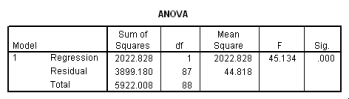
 What is the value of the correlation between body fat and body weight?
What is the value of the correlation between body fat and body weight? سؤال
A study was conducted to monitor the emissions of a noxious substance from a chemical plant and the concentration of the chemical at a location in close proximity to the plant at various times throughout the year.A total of 14 measurements were made.Computer output for the simple linear regression least-squares fit is provided.(Some entries have been omitted and replaced with **. )  The degrees of freedom for SSM and SSE are,respectively,
A)DFM = 2 and DFE = 12.
B)DFM = 1 and DFE = 12.
C)DFM = 1 and DFE = 13.
D)DFM = 1 and DFE = 14.
E)DFM = 12 and DFE = 13.
The degrees of freedom for SSM and SSE are,respectively,A)DFM = 2 and DFE = 12.
B)DFM = 1 and DFE = 12.
C)DFM = 1 and DFE = 13.
D)DFM = 1 and DFE = 14.
E)DFM = 12 and DFE = 13.
سؤال
A study was conducted to monitor the emissions of a noxious substance from a chemical plant and the concentration of the chemical at a location in close proximity to the plant at various times throughout the year.A total of 14 measurements were made.Computer output for the simple linear regression least-squares fit is provided.(Some entries have been omitted and replaced with **. )  What is the test statistic and its value to test H0:
  = 0 against Ha:
  0?
0?
A)F = 46.2294
B)t = 6.80
C)t = 1.35
D)F = 3.8524
E)Either A or B
What is the test statistic and its value to test H0: = 0 against Ha: 0?A)F = 46.2294
B)t = 6.80
C)t = 1.35
D)F = 3.8524
E)Either A or B
سؤال
A study was conducted to monitor the emissions of a noxious substance from a chemical plant and the concentration of the chemical at a location in close proximity to the plant at various times throughout the year.A total of 14 measurements were made.Computer output for the simple linear regression least-squares fit is provided.(Some entries have been omitted and replaced with **. ) 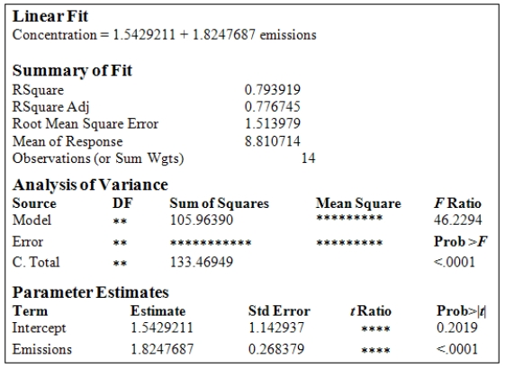 What is the value for the SSE?
A)27.50559
B)10.26688
C)1.142937
D)2.292
E)This cannot be determined with the information provided.
What is the value for the SSE?A)27.50559
B)10.26688
C)1.142937
D)2.292
E)This cannot be determined with the information provided.
سؤال
In the National Football League (NFL),having an effective passing game is seen to be important in order to win games.The following information for the 32 NFL teams in the 2007 season concerns the points a team scores per game (Pts/Gm)and the percent of its passes that were completed (Pass%).The ANOVA table is provided for the simple linear regression fit of Pts/Gm on Pass%.(Some entries have been omitted and replaced with **).  From the computer output for the least-squares fit,the following results were given:
  ,
,  = 0.3786,and
  = 4.001.Also,it was determined that
  = 61.05%,
  = 425.28,
  = 11.865,and
  = 0.194. What is the standard error of the estimated Pts/Gm for a team that completed 60% of its passes?
A)1.034
B)1.017
C)0.707
D)4.068
E)0.194
From the computer output for the least-squares fit,the following results were given: , = 0.3786,and = 4.001.Also,it was determined that = 61.05%, = 425.28, = 11.865,and = 0.194. What is the standard error of the estimated Pts/Gm for a team that completed 60% of its passes?A)1.034
B)1.017
C)0.707
D)4.068
E)0.194
سؤال
For the 2009 NFL season,data are available on such variables as the total yards gained by passing and by rushing for each of the 32 teams.The following is a scatter plot of the two variables,PassYds and RushYds. 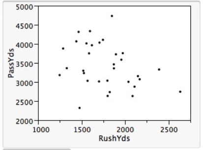 It was found that the correlation between the two variables was r = -0.313.In a test of hypothesis of H0: = 0 against Ha: 0,with = 0.05,the value of the test statistic and its degrees of freedom are,respectively,
A)t = -1.81 anddf = 31.
B)t = -2.04 and df = 30.
C)t = -2.04 and df = 31.
D)t = -1.81 and df = 30.
E)This cannot be determined without knowing SSM and SST.
It was found that the correlation between the two variables was r = -0.313.In a test of hypothesis of H0: = 0 against Ha: 0,with = 0.05,the value of the test statistic and its degrees of freedom are,respectively,A)t = -1.81 anddf = 31.
B)t = -2.04 and df = 30.
C)t = -2.04 and df = 31.
D)t = -1.81 and df = 30.
E)This cannot be determined without knowing SSM and SST.
سؤال
A recent study was done to assess factors that put Hispanic populations more at risk for obesity and related chronic diseases,such as diabetes and heart disease,than non-Hispanic populations.Data were collected on several factors,such as the crude morality rate of Hispanics,obesity prevalence,percent of adults diagnosed with diabetes,and median income at the state level.Pearson's Correlations were used to examine the strength of the relationship between obesity and the other variables,as a way of observing which characteristics were associated with high prevalence of obesity.In addition,a simple linear regression was used to model the relationship between diabetes and obesity.The results from SPSS are shown below. 


 What is the standard error of the slope b1 of the least-squares regression line for predicting obesity rates from diabetes rates?
A)1.43
B).135
C)1.34
D)None of the above
What is the standard error of the slope b1 of the least-squares regression line for predicting obesity rates from diabetes rates?A)1.43
B).135
C)1.34
D)None of the above
سؤال
A recent study was done to assess factors that put Hispanic populations more at risk for obesity and related chronic diseases,such as diabetes and heart disease,than non-Hispanic populations.Data were collected on several factors,such as the crude morality rate of Hispanics,obesity prevalence,percent of adults diagnosed with diabetes,and median income at the state level.Pearson's Correlations were used to examine the strength of the relationship between obesity and the other variables,as a way of observing which characteristics were associated with high prevalence of obesity.In addition,a simple linear regression was used to model the relationship between diabetes and obesity.The results from SPSS are shown below. 


 The largest diabetes rate is 14%.What is the predicted obesity rate?
A)0
B)1.43
C)50.2
D)None of the above
The largest diabetes rate is 14%.What is the predicted obesity rate?A)0
B)1.43
C)50.2
D)None of the above
سؤال
A recent study was done to assess factors that put Hispanic populations more at risk for obesity and related chronic diseases,such as diabetes and heart disease,than non-Hispanic populations.Data were collected on several factors,such as the crude morality rate of Hispanics,obesity prevalence,percent of adults diagnosed with diabetes,and median income at the state level.Pearson's Correlations were used to examine the strength of the relationship between obesity and the other variables,as a way of observing which characteristics were associated with high prevalence of obesity.In addition,a simple linear regression was used to model the relationship between diabetes and obesity.The results from SPSS are shown below. 


 What is the residual when the diabetes rate is 14%?
A)-1.67
B)32
C)It cannot be determined from the information given.
D)None of the above
What is the residual when the diabetes rate is 14%?A)-1.67
B)32
C)It cannot be determined from the information given.
D)None of the above
سؤال
A recent study was done to assess factors that put Hispanic populations more at risk for obesity and related chronic diseases,such as diabetes and heart disease,than non-Hispanic populations.Data were collected on several factors,such as the crude morality rate of Hispanics,obesity prevalence,percent of adults diagnosed with diabetes,and median income at the state level.Pearson's Correlations were used to examine the strength of the relationship between obesity and the other variables,as a way of observing which characteristics were associated with high prevalence of obesity.In addition,a simple linear regression was used to model the relationship between diabetes and obesity.The results from SPSS are shown below. 


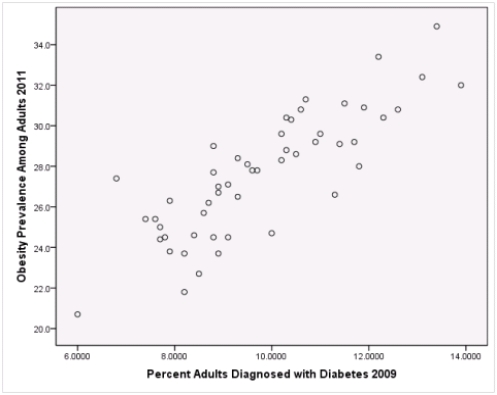 Based on the results,is there a statistically significant relationship between diabetes and obesity rates?
A)Yes,the scatterplot shows a strong linear relationship,and the ANOVA model for testing that the slope of the regression line is zero versus the alternative that the slope is not zero is statistically significant.
B)You cannot tell because the preliminary analysis of the data indicate that there is not a strong enough relationship between obesity rates and diabetes rates to trust the results of the ANOVA modelfor testing the slope of the regression line is zero versus the alternative that the slope is not zero.
C)No,simple linear regression is not the appropriate statistical procedure for these data.Therefore,the results are incorrect.
Based on the results,is there a statistically significant relationship between diabetes and obesity rates?A)Yes,the scatterplot shows a strong linear relationship,and the ANOVA model for testing that the slope of the regression line is zero versus the alternative that the slope is not zero is statistically significant.
B)You cannot tell because the preliminary analysis of the data indicate that there is not a strong enough relationship between obesity rates and diabetes rates to trust the results of the ANOVA modelfor testing the slope of the regression line is zero versus the alternative that the slope is not zero.
C)No,simple linear regression is not the appropriate statistical procedure for these data.Therefore,the results are incorrect.

فتح الحزمة
قم بالتسجيل لفتح البطاقات في هذه المجموعة!
Unlock Deck
Unlock Deck
1/91
العب
ملء الشاشة (f)
Deck 10: Inference for Regression
1
There is an old saying in golf: "You drive for show and you putt for dough." The point is that good putting is more important than long driving for shooting low scores and hence winning money.To see if this is the case,data on the top 69 money winners on the PGA tour in 1993 are examined.The average number of putts per hole for each player is used to predict the total winnings (in thousands of dollars)using the simple linear regression model (1993 winnings)i = 0 + 1(average number of putts per hole)i + i,
Where the deviations i are assumed to be independent and Normally distributed with a mean of 0 and a standard deviation of .This model was fit to the data using the method of least squares.The following results were obtained from statistical software. Suppose the researchers conducting this study wish to estimate the 1993 winnings when the average number of putts per hole is 1.75.The following results were obtained from statistical software. If the researchers wish to estimate the mean winnings for all tour pros whose average number of putts per hole is 1.75,what would be a 95% confidence interval for the mean winnings?
A)(77.7,1229.4)
B)(530.6,776.6)
C)653.6 ± 61.62
D)653.6 ± 123.24
Where the deviations i are assumed to be independent and Normally distributed with a mean of 0 and a standard deviation of .This model was fit to the data using the method of least squares.The following results were obtained from statistical software.
Suppose the researchers conducting this study wish to estimate the 1993 winnings when the average number of putts per hole is 1.75.The following results were obtained from statistical software. If the researchers wish to estimate the mean winnings for all tour pros whose average number of putts per hole is 1.75,what would be a 95% confidence interval for the mean winnings?A)(77.7,1229.4)
B)(530.6,776.6)
C)653.6 ± 61.62
D)653.6 ± 123.24
(530.6,776.6)
2
Which of the following statements about simple linear regression is/are FALSE?
A)The term "residual" refers to the difference between the observed response and the predicted response using the regression equation.
B)If and
are the intercept and slope,respectively,of the least-squares line,
is an unbiased estimator of the mean response when
.
C)The estimate of is given by s = .
D)The sum to zero.
A)The term "residual" refers to the difference between the observed response and the predicted response using the regression equation.
B)If
and are the intercept and slope,respectively,of the least-squares line, is an unbiased estimator of the mean response when .C)The estimate of is given by s =
.D)The
sum to zero. The estimate of is given by s = .
. 3
There is an old saying in golf: "You drive for show and you putt for dough." The point is that good putting is more important than long driving for shooting low scores and hence winning money.To see if this is the case,data on the top 69 money winners on the PGA tour in 1993 are examined.The average number of putts per hole for each player is used to predict the total winnings (in thousands of dollars)using the simple linear regression model (1993 winnings)i = 0 + 1(average number of putts per hole)i + i,
Where the deviations i are assumed to be independent and Normally distributed with a mean of 0 and a standard deviation of .This model was fit to the data using the method of least squares.The following results were obtained from statistical software. What is the value of the intercept of the least-squares regression line?
A)1698.4
B)3023.8
C)-4139.2
D)7897.2
Where the deviations i are assumed to be independent and Normally distributed with a mean of 0 and a standard deviation of .This model was fit to the data using the method of least squares.The following results were obtained from statistical software.
What is the value of the intercept of the least-squares regression line?A)1698.4
B)3023.8
C)-4139.2
D)7897.2
7897.2
4
There is an old saying in golf: "You drive for show and you putt for dough." The point is that good putting is more important than long driving for shooting low scores and hence winning money.To see if this is the case,data on the top 69 money winners on the PGA tour in 1993 are examined.The average number of putts per hole for each player is used to predict the total winnings (in thousands of dollars)using the simple linear regression model (1993 winnings)i = 0 + 1(average number of putts per hole)i + i,
Where the deviations i are assumed to be independent and Normally distributed with a mean of 0 and a standard deviation of .This model was fit to the data using the method of least squares.The following results were obtained from statistical software. The quantity s = 281.8 is an estimate of the standard deviation of the deviations in the simple linear regression model.What are the degrees of freedom for this estimate?
A)66
B)67
C)68
D)69
Where the deviations i are assumed to be independent and Normally distributed with a mean of 0 and a standard deviation of .This model was fit to the data using the method of least squares.The following results were obtained from statistical software.
The quantity s = 281.8 is an estimate of the standard deviation of the deviations in the simple linear regression model.What are the degrees of freedom for this estimate?A)66
B)67
C)68
D)69
فتح الحزمة
افتح القفل للوصول البطاقات البالغ عددها 91 في هذه المجموعة.
فتح الحزمة
k this deck
5
The statistical model for simple linear regression has the form ,i = 1,2,…,n.Which of the following statements about this statistical model is/are TRUE?
A)The are assumed to be Normally distributed with a mean of 0 and a standard deviation of .
B)The parameters of this model are ,
,and .
C) is the mean response when .
D)The ,i = 1,2,…,n are independent.
E)All of the above are true.
,i = 1,2,…,n.Which of the following statements about this statistical model is/are TRUE?A)The
are assumed to be Normally distributed with a mean of 0 and a standard deviation of .B)The parameters of this model are
, ,and .C)
is the mean response when .D)The
,i = 1,2,…,n are independent.E)All of the above are true.
فتح الحزمة
افتح القفل للوصول البطاقات البالغ عددها 91 في هذه المجموعة.
فتح الحزمة
k this deck
6
There is an old saying in golf: "You drive for show and you putt for dough." The point is that good putting is more important than long driving for shooting low scores and hence winning money.To see if this is the case,data on the top 69 money winners on the PGA tour in 1993 are examined.The average number of putts per hole for each player is used to predict the total winnings (in thousands of dollars)using the simple linear regression model (1993 winnings)i = 0 + 1(average number of putts per hole)i + i,
Where the deviations i are assumed to be independent and Normally distributed with a mean of 0 and a standard deviation of .This model was fit to the data using the method of least squares.The following results were obtained from statistical software. The following (partial)ANOVA table was obtained from statistical software. What is the value of the F statistic for testing the hypotheses H0: 1 = 0 versus Ha: 1 0?
A)0.089
B)2.44
C)4.72
D)5.94
Where the deviations i are assumed to be independent and Normally distributed with a mean of 0 and a standard deviation of .This model was fit to the data using the method of least squares.The following results were obtained from statistical software.
The following (partial)ANOVA table was obtained from statistical software. What is the value of the F statistic for testing the hypotheses H0: 1 = 0 versus Ha: 1 0?A)0.089
B)2.44
C)4.72
D)5.94
فتح الحزمة
افتح القفل للوصول البطاقات البالغ عددها 91 في هذه المجموعة.
فتح الحزمة
k this deck
7
There is an old saying in golf: "You drive for show and you putt for dough." The point is that good putting is more important than long driving for shooting low scores and hence winning money.To see if this is the case,data on the top 69 money winners on the PGA tour in 1993 are examined.The average number of putts per hole for each player is used to predict the total winnings (in thousands of dollars)using the simple linear regression model (1993 winnings)i = 0 + 1(average number of putts per hole)i + i,
Where the deviations i are assumed to be independent and Normally distributed with a mean of 0 and a standard deviation of .This model was fit to the data using the method of least squares.The following results were obtained from statistical software. Suppose the researchers conducting this study wish to test the hypotheses H0: 1 = 0 versus Ha: 1< 0.What is the value of the t statistic for this test?
A)-2.44
B)-1.91
C)2.44
D)2.61
Where the deviations i are assumed to be independent and Normally distributed with a mean of 0 and a standard deviation of .This model was fit to the data using the method of least squares.The following results were obtained from statistical software.
Suppose the researchers conducting this study wish to test the hypotheses H0: 1 = 0 versus Ha: 1< 0.What is the value of the t statistic for this test?A)-2.44
B)-1.91
C)2.44
D)2.61
فتح الحزمة
افتح القفل للوصول البطاقات البالغ عددها 91 في هذه المجموعة.
فتح الحزمة
k this deck
8
There is an old saying in golf: "You drive for show and you putt for dough." The point is that good putting is more important than long driving for shooting low scores and hence winning money.To see if this is the case,data on the top 69 money winners on the PGA tour in 1993 are examined.The average number of putts per hole for each player is used to predict the total winnings (in thousands of dollars)using the simple linear regression model (1993 winnings)i = 0 + 1(average number of putts per hole)i + i,
Where the deviations i are assumed to be independent and Normally distributed with a mean of 0 and a standard deviation of .This model was fit to the data using the method of least squares.The following results were obtained from statistical software. Which of the following conclusions seems most justified?
A)There is no evidence of a relation between the average number of putts per round and the 1993 winnings of PGA tour pros.
B)There is distinct evidence (P-value less than 0.05)that there is a positive correlation between 1993 winnings and average number of putts per round.
C)There is some evidence that PGA tour pros who averaged fewer putts per round had higher winnings in 1993.
D)The presence of strongly influential observations in these data makes it impossible to draw any conclusions about the relationship between 1993 winnings and average number of putts per round.
Where the deviations i are assumed to be independent and Normally distributed with a mean of 0 and a standard deviation of .This model was fit to the data using the method of least squares.The following results were obtained from statistical software.
Which of the following conclusions seems most justified?A)There is no evidence of a relation between the average number of putts per round and the 1993 winnings of PGA tour pros.
B)There is distinct evidence (P-value less than 0.05)that there is a positive correlation between 1993 winnings and average number of putts per round.
C)There is some evidence that PGA tour pros who averaged fewer putts per round had higher winnings in 1993.
D)The presence of strongly influential observations in these data makes it impossible to draw any conclusions about the relationship between 1993 winnings and average number of putts per round.
فتح الحزمة
افتح القفل للوصول البطاقات البالغ عددها 91 في هذه المجموعة.
فتح الحزمة
k this deck
9
Do heavier cars use more gasoline? To answer this question,a researcher randomly selected 15 cars.He collected their weight (in hundreds of pounds)and the mileage (MPG)for each car.From a scatter plot made with the data,a linear model seemed appropriate.The following output was obtained from SPSS: What is the equation of the least-squares regression line?
A)ŷ = -0.52 x + 0.164
B)ŷ = 40.44 - 0.52x
C)ŷ = 40.44 + 6.28x
D)y = 40.44 + 0.52x
What is the equation of the least-squares regression line?A)ŷ = -0.52 x + 0.164
B)ŷ = 40.44 - 0.52x
C)ŷ = 40.44 + 6.28x
D)y = 40.44 + 0.52x
فتح الحزمة
افتح القفل للوصول البطاقات البالغ عددها 91 في هذه المجموعة.
فتح الحزمة
k this deck
10
There is an old saying in golf: "You drive for show and you putt for dough." The point is that good putting is more important than long driving for shooting low scores and hence winning money.To see if this is the case,data on the top 69 money winners on the PGA tour in 1993 are examined.The average number of putts per hole for each player is used to predict the total winnings (in thousands of dollars)using the simple linear regression model (1993 winnings)i = 0 + 1(average number of putts per hole)i + i,
Where the deviations i are assumed to be independent and Normally distributed with a mean of 0 and a standard deviation of .This model was fit to the data using the method of least squares.The following results were obtained from statistical software. What is an approximate 95% confidence interval for the slope 1?
A)-4139.2 ± 1698.2
B)-4139.2 ± 3396.4
C)7897.2 ± 3023.8
D)7897.2 ± 6047.6
Where the deviations i are assumed to be independent and Normally distributed with a mean of 0 and a standard deviation of .This model was fit to the data using the method of least squares.The following results were obtained from statistical software.
What is an approximate 95% confidence interval for the slope 1?A)-4139.2 ± 1698.2
B)-4139.2 ± 3396.4
C)7897.2 ± 3023.8
D)7897.2 ± 6047.6
فتح الحزمة
افتح القفل للوصول البطاقات البالغ عددها 91 في هذه المجموعة.
فتح الحزمة
k this deck
11
The data referred to in this question were collected on 41 employees of a large company.The company is trying to predict the current salary of its employees from their starting salary (both expressed in thousands of dollars).The SPSS regression output is given below as well as some summary measures: What is the value of the estimate for ,the standard deviation of the model deviations i?
A)0.15
B)2.93
C)7.21
D)52.0
What is the value of the estimate for ,the standard deviation of the model deviations i?A)0.15
B)2.93
C)7.21
D)52.0
فتح الحزمة
افتح القفل للوصول البطاقات البالغ عددها 91 في هذه المجموعة.
فتح الحزمة
k this deck
12
Do heavier cars use more gasoline? To answer this question,a researcher randomly selected 15 cars.He collected their weight (in hundreds of pounds)and the mileage (MPG)for each car.From a scatter plot made with the data,a linear model seemed appropriate.The following output was obtained from SPSS: To test if there is a significant straight-line relationship between the weight and the mileage of a car,we can perform a t test.What is the value of the t statistic for this test?
A)t = -3.182
B)t = 6.445
C)t = 6.780
D)This cannot be determined from the information given.
To test if there is a significant straight-line relationship between the weight and the mileage of a car,we can perform a t test.What is the value of the t statistic for this test?A)t = -3.182
B)t = 6.445
C)t = 6.780
D)This cannot be determined from the information given.
فتح الحزمة
افتح القفل للوصول البطاقات البالغ عددها 91 في هذه المجموعة.
فتح الحزمة
k this deck
13
Which of the following statements about the simple linear regression model and its least squares fit is/are FALSE?
A)The ANOVA table gives degrees of freedom,sum of squares,and mean squares for the model,error,and total sources of variation.
B)The ANOVA F statistic is the ratio MSM/MSE.
C)The ANOVA F statistic has an F(1,n - 2)under the null hypothesis H0:
= 0.
D)The ANOVA F statistic is particularly useful because it tests the H0: = 0 against the one-sided alternative Ha:
> 0.
E)The ratio SSM/SST is equal to .
A)The ANOVA table gives degrees of freedom,sum of squares,and mean squares for the model,error,and total sources of variation.
B)The ANOVA F statistic is the ratio MSM/MSE.
C)The ANOVA F statistic has an F(1,n - 2)under the null hypothesis H0:
= 0.
D)The ANOVA F statistic is particularly useful because it tests the H0:
= 0 against the one-sided alternative Ha: > 0.
E)The ratio SSM/SST is equal to
. فتح الحزمة
افتح القفل للوصول البطاقات البالغ عددها 91 في هذه المجموعة.
فتح الحزمة
k this deck
14
There is an old saying in golf: "You drive for show and you putt for dough." The point is that good putting is more important than long driving for shooting low scores and hence winning money.To see if this is the case,data on the top 69 money winners on the PGA tour in 1993 are examined.The average number of putts per hole for each player is used to predict the total winnings (in thousands of dollars)using the simple linear regression model (1993 winnings)i = 0 + 1(average number of putts per hole)i + i,
Where the deviations i are assumed to be independent and Normally distributed with a mean of 0 and a standard deviation of .This model was fit to the data using the method of least squares.The following results were obtained from statistical software. Suppose the researchers conducting this study wish to estimate the 1993 winnings when the average number of putts per hole is 1.75.The following results were obtained from statistical software. If the researchers wish to estimate the winnings for a particular tour pro whose average number of putts per hole is 1.75,what would be a 95% prediction interval for the winnings?
A)(77.7,1229.4)
B)(530.6,776.6)
C)653.6 ± 61.62
D)653.6 ± 123.24
Where the deviations i are assumed to be independent and Normally distributed with a mean of 0 and a standard deviation of .This model was fit to the data using the method of least squares.The following results were obtained from statistical software.
Suppose the researchers conducting this study wish to estimate the 1993 winnings when the average number of putts per hole is 1.75.The following results were obtained from statistical software. If the researchers wish to estimate the winnings for a particular tour pro whose average number of putts per hole is 1.75,what would be a 95% prediction interval for the winnings?A)(77.7,1229.4)
B)(530.6,776.6)
C)653.6 ± 61.62
D)653.6 ± 123.24
فتح الحزمة
افتح القفل للوصول البطاقات البالغ عددها 91 في هذه المجموعة.
فتح الحزمة
k this deck
15
There is an old saying in golf: "You drive for show and you putt for dough." The point is that good putting is more important than long driving for shooting low scores and hence winning money.To see if this is the case,data on the top 69 money winners on the PGA tour in 1993 are examined.The average number of putts per hole for each player is used to predict the total winnings (in thousands of dollars)using the simple linear regression model (1993 winnings)i = 0 + 1(average number of putts per hole)i + i,
Where the deviations i are assumed to be independent and Normally distributed with a mean of 0 and a standard deviation of .This model was fit to the data using the method of least squares.The following results were obtained from statistical software. The following (partial)ANOVA table was obtained from statistical software. What is the value of the SST,the total sum of squares?
A)79,398
B)471,605
C)5,319,690
D)5,791,295
Where the deviations i are assumed to be independent and Normally distributed with a mean of 0 and a standard deviation of .This model was fit to the data using the method of least squares.The following results were obtained from statistical software.
The following (partial)ANOVA table was obtained from statistical software. What is the value of the SST,the total sum of squares?A)79,398
B)471,605
C)5,319,690
D)5,791,295
فتح الحزمة
افتح القفل للوصول البطاقات البالغ عددها 91 في هذه المجموعة.
فتح الحزمة
k this deck
16
Do heavier cars use more gasoline? To answer this question,a researcher randomly selected 15 cars.He collected their weight (in hundreds of pounds)and the mileage (MPG)for each car.From a scatter plot made with the data,a linear model seemed appropriate.The following output was obtained from SPSS: Which of the following descriptions of the value of the slope is the correct description?
A)We cannot interpret the slope because we cannot have a negative weight of a car.
B)We estimate the mileage to decrease by 0.521 miles per gallon when the weight of a car increases by 1 pound.
C)We estimate the mileage to decrease by 0.521 miles per gallon when the weight of a car increases by 100 pounds.
D)We estimate the mileage to decrease by 52.1 miles per gallon when the weight of a car increases by 100 pounds.
Which of the following descriptions of the value of the slope is the correct description?A)We cannot interpret the slope because we cannot have a negative weight of a car.
B)We estimate the mileage to decrease by 0.521 miles per gallon when the weight of a car increases by 1 pound.
C)We estimate the mileage to decrease by 0.521 miles per gallon when the weight of a car increases by 100 pounds.
D)We estimate the mileage to decrease by 52.1 miles per gallon when the weight of a car increases by 100 pounds.
فتح الحزمة
افتح القفل للوصول البطاقات البالغ عددها 91 في هذه المجموعة.
فتح الحزمة
k this deck
17
The data referred to in this question were collected on 41 employees of a large company.The company is trying to predict the current salary of its employees from their starting salary (both expressed in thousands of dollars).The SPPS regression output is given below as well as some summary measures: What is an approximate 95% confidence interval for the slope 1?
A)(-7.57,4.39)
B)(-4.52,1.34)
C)(1.80,2.41)
D)(1.95,2.26)
What is an approximate 95% confidence interval for the slope 1?A)(-7.57,4.39)
B)(-4.52,1.34)
C)(1.80,2.41)
D)(1.95,2.26)
فتح الحزمة
افتح القفل للوصول البطاقات البالغ عددها 91 في هذه المجموعة.
فتح الحزمة
k this deck
18
The data referred to in this question were collected on 41 employees of a large company.The company is trying to predict the current salary of its employees from their starting salary (both expressed in thousands of dollars).The SPPS regression output is given below as well as some summary measures: Suppose we wish to test the hypotheses H0: 1 = 2 versus Ha: 1 2.Together with an insignificant constant in this model,this would imply that the employees currently earn about twice as much as their starting salary.At the 5% significance level,would we reject the null hypothesis?
A)Yes
B)No
C)This cannot be determined from the information given.
Suppose we wish to test the hypotheses H0: 1 = 2 versus Ha: 1 2.Together with an insignificant constant in this model,this would imply that the employees currently earn about twice as much as their starting salary.At the 5% significance level,would we reject the null hypothesis?A)Yes
B)No
C)This cannot be determined from the information given.
فتح الحزمة
افتح القفل للوصول البطاقات البالغ عددها 91 في هذه المجموعة.
فتح الحزمة
k this deck
19
The data referred to in this question were collected on 41 employees of a large company.The company is trying to predict the current salary of its employees from their starting salary (both expressed in thousands of dollars).The SPSS regression output is given below as well as some summary measures: How would a 90% confidence interval for the average current salary for all employees who started with a salary of $15,300 compare to a 90% confidence interval for the current salary of an individual with a starting salary of $15,300?
A)It would be narrower.
B)It would be the same.
C)It would be wider.
D)This cannot be determined from the information given.
How would a 90% confidence interval for the average current salary for all employees who started with a salary of $15,300 compare to a 90% confidence interval for the current salary of an individual with a starting salary of $15,300?A)It would be narrower.
B)It would be the same.
C)It would be wider.
D)This cannot be determined from the information given.
فتح الحزمة
افتح القفل للوصول البطاقات البالغ عددها 91 في هذه المجموعة.
فتح الحزمة
k this deck
20
The data referred to in this question were collected on 41 employees of a large company.The company is trying to predict the current salary of its employees from their starting salary (both expressed in thousands of dollars).The SPSS regression output is given below as well as some summary measures: John Doe works for this company.He started with a salary of $15,300.Predict his current salary with a 90% confidence interval.Express the interval in the appropriate units.
A)($15,683;$45,537)
B)($18,204;$43,015)
C)($28,580;$32,640)
D)($31,516;$32,885)
John Doe works for this company.He started with a salary of $15,300.Predict his current salary with a 90% confidence interval.Express the interval in the appropriate units.A)($15,683;$45,537)
B)($18,204;$43,015)
C)($28,580;$32,640)
D)($31,516;$32,885)
فتح الحزمة
افتح القفل للوصول البطاقات البالغ عددها 91 في هذه المجموعة.
فتح الحزمة
k this deck
21
The statistical model for simple linear regression is written as ,where represents the mean of a Normally distributed response variable and x represents the explanatory variable.The parameters and are estimated,giving the linear regression model defined by ,with standard deviation = 5. What is the y-intercept for the regression line?
A)10
B)70
C)80
D)60
,where represents the mean of a Normally distributed response variable and x represents the explanatory variable.The parameters and are estimated,giving the linear regression model defined by ,with standard deviation = 5. What is the y-intercept for the regression line?A)10
B)70
C)80
D)60
فتح الحزمة
افتح القفل للوصول البطاقات البالغ عددها 91 في هذه المجموعة.
فتح الحزمة
k this deck
22
A random sample of 79 companies from the Forbes 500 list (which actually consists of nearly 800 companies)was selected,and the relationship between sales (in hundreds of thousands of dollars)and profits (in hundreds of thousands of dollars)was investigated by regression.The following results were obtained from statistical software. The following (partial)ANOVA table was obtained from statistical software. What is the value of the SST,the total sum of squares?
A)16,074,978
B)16,734,234
C)32,809,212
D)49,543,448
The following (partial)ANOVA table was obtained from statistical software. What is the value of the SST,the total sum of squares?A)16,074,978
B)16,734,234
C)32,809,212
D)49,543,448
فتح الحزمة
افتح القفل للوصول البطاقات البالغ عددها 91 في هذه المجموعة.
فتح الحزمة
k this deck
23
A random sample of 79 companies from the Forbes 500 list (which actually consists of nearly 800 companies)was selected,and the relationship between sales (in hundreds of thousands of dollars)and profits (in hundreds of thousands of dollars)was investigated by regression.The following results were obtained from statistical software. What is approximately the value of the intercept of the least-squares regression line?
A)0.0075
B)0.0925
C)61.16
D)-176.64
What is approximately the value of the intercept of the least-squares regression line?A)0.0075
B)0.0925
C)61.16
D)-176.64
فتح الحزمة
افتح القفل للوصول البطاقات البالغ عددها 91 في هذه المجموعة.
فتح الحزمة
k this deck
24
As in most professional sports,statistics are collected in the National Hockey League.In the 2006-2007 season,teams played 82 games.A team was awarded 2 points for a win and 1 point if the game was tied at the end of regulation time but then lost in overtime.For each of the 30 teams,data on the number of goals scored per game (Goals/G)and the percentage of the 164 possible points they won (Win%)during the season were collected.The following graph shows the plotted points for the variables Win% and Goals/G and the simple linear regression line fitted using least squares. From the computer output for the least-squares fit,the estimated equation was found to be , = 0.398,and = 60.29.Also,it was determined from the output that = 12.800 and = 4.418. Which of the following statements is/are FALSE?
A)An amount of 39.8% of the variation in the winning percent variable is explained by the least-squares regression on the number of goals scored per game.
B)An increase of 1 goal per game results in an increase of about 19% in winning percent.
C)If a team scores 3 goals per game,we would predict the team would have a Win% of 55%.
D)The Ottawa Senators scored 3.49 goals per game and their Win% was 64.0.The residual for Ottawa was then -3.32.
E)The mean value of the Win% variable is 0.932 when the Goals/G is 0.
From the computer output for the least-squares fit,the estimated equation was found to be , = 0.398,and = 60.29.Also,it was determined from the output that = 12.800 and = 4.418. Which of the following statements is/are FALSE?A)An amount of 39.8% of the variation in the winning percent variable is explained by the least-squares regression on the number of goals scored per game.
B)An increase of 1 goal per game results in an increase of about 19% in winning percent.
C)If a team scores 3 goals per game,we would predict the team would have a Win% of 55%.
D)The Ottawa Senators scored 3.49 goals per game and their Win% was 64.0.The residual for Ottawa was then -3.32.
E)The mean value of the Win% variable is 0.932 when the Goals/G is 0.
فتح الحزمة
افتح القفل للوصول البطاقات البالغ عددها 91 في هذه المجموعة.
فتح الحزمة
k this deck
25
A random sample of 79 companies from the Forbes 500 list (which actually consists of nearly 800 companies)was selected,and the relationship between sales (in hundreds of thousands of dollars)and profits (in hundreds of thousands of dollars)was investigated by regression.The following results were obtained from statistical software. Suppose the researchers conducting the study wish to test the hypotheses H0: 1 = 0 versus Ha: 1> 0.What do we know about the P-value of this test?
A)The P-value is greater than 0.10.
B)The P-value is between 0.05 and 0.10.
C)The P-value is between 0.01 and 0.05.
D)The P-value is less than 0.01.
Suppose the researchers conducting the study wish to test the hypotheses H0: 1 = 0 versus Ha: 1> 0.What do we know about the P-value of this test?A)The P-value is greater than 0.10.
B)The P-value is between 0.05 and 0.10.
C)The P-value is between 0.01 and 0.05.
D)The P-value is less than 0.01.
فتح الحزمة
افتح القفل للوصول البطاقات البالغ عددها 91 في هذه المجموعة.
فتح الحزمة
k this deck
26
A random sample of 79 companies from the Forbes 500 list (which actually consists of nearly 800 companies)was selected,and the relationship between sales (in hundreds of thousands of dollars)and profits (in hundreds of thousands of dollars)was investigated by regression.The following results were obtained from statistical software. The following (partial)ANOVA table was obtained from statistical software. What is the value of the F statistic for testing the hypotheses H0: 1 = 0 versus Ha: 1 0?
A)1.96
B)77
C)150.97
D)217,328
The following (partial)ANOVA table was obtained from statistical software. What is the value of the F statistic for testing the hypotheses H0: 1 = 0 versus Ha: 1 0?A)1.96
B)77
C)150.97
D)217,328
فتح الحزمة
افتح القفل للوصول البطاقات البالغ عددها 91 في هذه المجموعة.
فتح الحزمة
k this deck
27
A random sample of 79 companies from the Forbes 500 list (which actually consists of nearly 800 companies)was selected,and the relationship between sales (in hundreds of thousands of dollars)and profits (in hundreds of thousands of dollars)was investigated by regression.The following results were obtained from statistical software. What is an approximate 90% confidence interval for the slope 1?
A)-0.09 ± 0.0075
B)-0.09 ± 0.0125
C)0.09 ± 0.0075
D)0.09 ± 0.0125
What is an approximate 90% confidence interval for the slope 1?A)-0.09 ± 0.0075
B)-0.09 ± 0.0125
C)0.09 ± 0.0075
D)0.09 ± 0.0125
فتح الحزمة
افتح القفل للوصول البطاقات البالغ عددها 91 في هذه المجموعة.
فتح الحزمة
k this deck
28
The statistical model for simple linear regression is written as ,where represents the mean of a Normally distributed response variable and x represents the explanatory variable.The parameters and are estimated,giving the linear regression model defined by ,with standard deviation = 5. What is the slope of the regression line?
A)10
B)70
C)80
D)60
,where represents the mean of a Normally distributed response variable and x represents the explanatory variable.The parameters and are estimated,giving the linear regression model defined by ,with standard deviation = 5. What is the slope of the regression line?A)10
B)70
C)80
D)60
فتح الحزمة
افتح القفل للوصول البطاقات البالغ عددها 91 في هذه المجموعة.
فتح الحزمة
k this deck
29
A random sample of 79 companies from the Forbes 500 list (which actually consists of nearly 800 companies)was selected,and the relationship between sales (in hundreds of thousands of dollars)and profits (in hundreds of thousands of dollars)was investigated by regression.The following results were obtained from statistical software. The following (partial)ANOVA table was obtained from statistical software. What are the degrees of freedom for SSE,the error sum of squares?
A)2
B)77
C)78
D)79
The following (partial)ANOVA table was obtained from statistical software. What are the degrees of freedom for SSE,the error sum of squares?A)2
B)77
C)78
D)79
فتح الحزمة
افتح القفل للوصول البطاقات البالغ عددها 91 في هذه المجموعة.
فتح الحزمة
k this deck
30
As in most professional sports,statistics are collected in the National Hockey League.In the 2006-2007 season,teams played 82 games.A team was awarded 2 points for a win and 1 point if the game was tied at the end of regulation time but then lost in overtime.For each of the 30 teams,data on the number of goals scored per game (Goals/G)and the percentage of the 164 possible points they won (Win%)during the season were collected.The following graph shows the plotted points for the variables Win% and Goals/G and the simple linear regression line fitted using least squares. From the computer output for the least-squares fit,the estimated equation was found to be , = 0.398,and = 60.29.Also,it was determined from the output that = 12.800 and = 4.418. If a test of hypothesis were conducted of H0: = 0 against Ha: 0,what would be the value of the test statistic?
A)t = 0.07
B)z = 0.07
C)z = 4.31
D)F = 4.31
E)t = 4.31
From the computer output for the least-squares fit,the estimated equation was found to be , = 0.398,and = 60.29.Also,it was determined from the output that = 12.800 and = 4.418. If a test of hypothesis were conducted of H0: = 0 against Ha: 0,what would be the value of the test statistic?A)t = 0.07
B)z = 0.07
C)z = 4.31
D)F = 4.31
E)t = 4.31
فتح الحزمة
افتح القفل للوصول البطاقات البالغ عددها 91 في هذه المجموعة.
فتح الحزمة
k this deck
31
Do heavier cars use more gasoline? To answer this question,a researcher randomly selected 15 cars.He collected their weight (in hundreds of pounds)and the mileage (MPG)for each car.From a scatter plot made with the data,a linear model seemed appropriate.The following output was obtained from SPSS: What is a 95% confidence interval for the slope 1?
A)(-0.875,-0.167)
B)(-0.685,-0.357)
C)(-1.04,0.001)
D)(26.89,53.99)
What is a 95% confidence interval for the slope 1?A)(-0.875,-0.167)
B)(-0.685,-0.357)
C)(-1.04,0.001)
D)(26.89,53.99)
فتح الحزمة
افتح القفل للوصول البطاقات البالغ عددها 91 في هذه المجموعة.
فتح الحزمة
k this deck
32
A random sample of 79 companies from the Forbes 500 list (which actually consists of nearly 800 companies)was selected,and the relationship between sales (in hundreds of thousands of dollars)and profits (in hundreds of thousands of dollars)was investigated by regression.The following results were obtained from statistical software. Suppose the researchers conducting this study wish to estimate the profits (in hundreds of thousands of dollars)for companies that had sales (in hundreds of thousands of dollars)of 500.The following results were obtained from statistical software. If the researchers wish to estimate the profits for a particular company that had sales of 500,what would be a 95% prediction interval for the profits?
A)(-1066.4,805.6)
B)(-248.5,-12.3)
C)-130.4 ± 59.3
D)500 ± 59.3
Suppose the researchers conducting this study wish to estimate the profits (in hundreds of thousands of dollars)for companies that had sales (in hundreds of thousands of dollars)of 500.The following results were obtained from statistical software. If the researchers wish to estimate the profits for a particular company that had sales of 500,what would be a 95% prediction interval for the profits?A)(-1066.4,805.6)
B)(-248.5,-12.3)
C)-130.4 ± 59.3
D)500 ± 59.3
فتح الحزمة
افتح القفل للوصول البطاقات البالغ عددها 91 في هذه المجموعة.
فتح الحزمة
k this deck
33
As in most professional sports,statistics are collected in the National Hockey League.In the 2006-2007 season,teams played 82 games.A team was awarded 2 points for a win and 1 point if the game was tied at the end of regulation time but then lost in overtime.For each of the 30 teams,data on the number of goals scored per game (Goals/G)and the percentage of the 164 possible points they won (Win%)during the season were collected.The following graph shows the plotted points for the variables Win% and Goals/G and the simple linear regression line fitted using least squares. From the computer output for the least-squares fit,the estimated equation was found to be = 0.398,and = 60.29.Also,it was determined from the output that = 12.800 and = 4.418.For the 2006-2007 season,teams scored an average of = 2.88 goals per game.For the population of teams that score 2.5 goals per game,the standard error of the estimated mean Win% is = 2.197.What is the estimated mean Win% for the population of teams that score 2.5 goals per game?
A)42.7%
B)53.6%
C)48.5%
D)55.7%
E)Not within ± 2% of any of the above
From the computer output for the least-squares fit,the estimated equation was found to be = 0.398,and = 60.29.Also,it was determined from the output that = 12.800 and = 4.418.For the 2006-2007 season,teams scored an average of = 2.88 goals per game.For the population of teams that score 2.5 goals per game,the standard error of the estimated mean Win% is = 2.197.What is the estimated mean Win% for the population of teams that score 2.5 goals per game?A)42.7%
B)53.6%
C)48.5%
D)55.7%
E)Not within ± 2% of any of the above
فتح الحزمة
افتح القفل للوصول البطاقات البالغ عددها 91 في هذه المجموعة.
فتح الحزمة
k this deck
34
A random sample of 79 companies from the Forbes 500 list (which actually consists of nearly 800 companies)was selected,and the relationship between sales (in hundreds of thousands of dollars)and profits (in hundreds of thousands of dollars)was investigated by regression.The following results were obtained from statistical software. Suppose the researchers conducting this study wish to estimate the profits (in hundreds of thousands of dollars)for companies that had sales (in hundreds of thousands of dollars)of 500.The following results were obtained from statistical software. If the researchers wish to estimate the mean profits for all companies that had sales of 500,what would be a 95% confidence interval for the mean profits?
A)(-1066.4,805.6)
B)(-248.5,-12.3)
C)-130.4 ± 59.3
D)500 ± 59.3
Suppose the researchers conducting this study wish to estimate the profits (in hundreds of thousands of dollars)for companies that had sales (in hundreds of thousands of dollars)of 500.The following results were obtained from statistical software. If the researchers wish to estimate the mean profits for all companies that had sales of 500,what would be a 95% confidence interval for the mean profits?A)(-1066.4,805.6)
B)(-248.5,-12.3)
C)-130.4 ± 59.3
D)500 ± 59.3
فتح الحزمة
افتح القفل للوصول البطاقات البالغ عددها 91 في هذه المجموعة.
فتح الحزمة
k this deck
35
A random sample of 79 companies from the Forbes 500 list (which actually consists of nearly 800 companies)was selected,and the relationship between sales (in hundreds of thousands of dollars)and profits (in hundreds of thousands of dollars)was investigated by regression.The following results were obtained from statistical software. Is there strong evidence of a straight-line relationship between sales and profits? Explain briefly.
A)Yes,because the slope of the least-squares line is positive
B)Yes,because the P-value for testing if the slope is zero is quite small
C)No,because the value of the square of the correlation is relatively small
D)It is impossible to say because we are not given the actual value of the correlation.
Is there strong evidence of a straight-line relationship between sales and profits? Explain briefly.A)Yes,because the slope of the least-squares line is positive
B)Yes,because the P-value for testing if the slope is zero is quite small
C)No,because the value of the square of the correlation is relatively small
D)It is impossible to say because we are not given the actual value of the correlation.
فتح الحزمة
افتح القفل للوصول البطاقات البالغ عددها 91 في هذه المجموعة.
فتح الحزمة
k this deck
36
The statistical model for simple linear regression is written as ,where represents the mean of a Normally distributed response variable and x represents the explanatory variable.The parameters and are estimated,giving the linear regression model defined by ,with standard deviation = 5. The explanatory variable x is ________.
A)quantitative
B)qualitative
C)categorical
D)None of the above
,where represents the mean of a Normally distributed response variable and x represents the explanatory variable.The parameters and are estimated,giving the linear regression model defined by ,with standard deviation = 5. The explanatory variable x is ________.A)quantitative
B)qualitative
C)categorical
D)None of the above
فتح الحزمة
افتح القفل للوصول البطاقات البالغ عددها 91 في هذه المجموعة.
فتح الحزمة
k this deck
37
As in most professional sports,statistics are collected in the National Hockey League.In the 2006-2007 season,teams played 82 games.A team was awarded 2 points for a win and 1 point if the game was tied at the end of regulation time but then lost in overtime.For each of the 30 teams,data on the number of goals scored per game (Goals/G)and the percentage of the 164 possible points they won (Win%)during the season were collected.The following graph shows the plotted points for the variables Win% and Goals/G and the simple linear regression line fitted using least squares. From the computer output for the least-squares fit,the estimated equation was found to be , = 0.398,and = 60.29.Also,it was determined from the output that = 12.800 and = 4.418.We are told that = 60.29.How many degrees of freedom are associated with this statistic?
A)29
B)1
C)30
D)28
E)None of the above
From the computer output for the least-squares fit,the estimated equation was found to be , = 0.398,and = 60.29.Also,it was determined from the output that = 12.800 and = 4.418.We are told that = 60.29.How many degrees of freedom are associated with this statistic?A)29
B)1
C)30
D)28
E)None of the above
فتح الحزمة
افتح القفل للوصول البطاقات البالغ عددها 91 في هذه المجموعة.
فتح الحزمة
k this deck
38
As in most professional sports,statistics are collected in the National Hockey League.In the 2006-2007 season,teams played 82 games.A team was awarded 2 points for a win and 1 point if the game was tied at the end of regulation time but then lost in overtime.For each of the 30 teams,data on the number of goals scored per game (Goals/G)and the percentage of the 164 possible points they won (Win%)during the season were collected.The following graph shows the plotted points for the variables Win% and Goals/G and the simple linear regression line fitted using least squares. From the computer output for the least-squares fit,the estimated equation was found to be , = 0.398,and = 60.29.Also,it was determined from the output that = 12.800 and = 4.418. A plot of the residuals from the least-squares fit against the Goals/G variable is shown below. What statements about residuals and/or about this residual plot is/are FALSE?
A)There does not appear to be any particular pattern to the residuals on the plot.
B)The residual plot shows that the residuals do approximately follow a Normal distribution,as the statistical model requires.
C)Residuals from a least-squares fit in simple linear regression always sum to zero.
D)None of the residuals look as though they would be considered to be outliers.
E)The residuals appear to vary randomly about their mean of zero.
From the computer output for the least-squares fit,the estimated equation was found to be , = 0.398,and = 60.29.Also,it was determined from the output that = 12.800 and = 4.418. A plot of the residuals from the least-squares fit against the Goals/G variable is shown below. What statements about residuals and/or about this residual plot is/are FALSE?A)There does not appear to be any particular pattern to the residuals on the plot.
B)The residual plot shows that the residuals do approximately follow a Normal distribution,as the statistical model requires.
C)Residuals from a least-squares fit in simple linear regression always sum to zero.
D)None of the residuals look as though they would be considered to be outliers.
E)The residuals appear to vary randomly about their mean of zero.
فتح الحزمة
افتح القفل للوصول البطاقات البالغ عددها 91 في هذه المجموعة.
فتح الحزمة
k this deck
39
As in most professional sports,statistics are collected in the National Hockey League.In the 2006-2007 season,teams played 82 games.A team was awarded 2 points for a win and 1 point if the game was tied at the end of regulation time but then lost in overtime.For each of the 30 teams,data on the number of goals scored per game (Goals/G)and the percentage of the 164 possible points they won (Win%)during the season were collected.The following graph shows the plotted points for the variables Win% and Goals/G and the simple linear regression line fitted using least squares. From the computer output for the least-squares fit,the estimated equation was found to be , = 0.398,and = 60.29.Also,it was determined from the output that = 12.800 and = 4.418.What would the approximate 96% confidence interval be for the true slope ?
A)19.022 ± 2.054(12.800)
B)19.022 ± 2.154(4.418)
C)0.932 ± 2.154(12.800)
D)19.022 ± 2.054(4.418)
E)0.932 ± 2.154 (12.800)
From the computer output for the least-squares fit,the estimated equation was found to be , = 0.398,and = 60.29.Also,it was determined from the output that = 12.800 and = 4.418.What would the approximate 96% confidence interval be for the true slope ?A)19.022 ± 2.054(12.800)
B)19.022 ± 2.154(4.418)
C)0.932 ± 2.154(12.800)
D)19.022 ± 2.054(4.418)
E)0.932 ± 2.154 (12.800)
فتح الحزمة
افتح القفل للوصول البطاقات البالغ عددها 91 في هذه المجموعة.
فتح الحزمة
k this deck
40
The statistical model for linear regression can be expressed as which of the following equations?
A)DATA = FIT + RESIDUAL
B)FIT = DATA + RESIDUAL
C)RESIDUAL = DATA + FIT
D)DATA = FIT
A)DATA = FIT + RESIDUAL
B)FIT = DATA + RESIDUAL
C)RESIDUAL = DATA + FIT
D)DATA = FIT
فتح الحزمة
افتح القفل للوصول البطاقات البالغ عددها 91 في هذه المجموعة.
فتح الحزمة
k this deck
41
The statistical model for simple linear regression is written as ,where represents the mean of a Normally distributed response variable and x represents the explanatory variable.The parameters and are estimated,giving the linear regression model defined by ,with standard deviation = 5. What is the distribution of the test statistic used to test the null hypothesis against the alternative hypothesis ? (Note: Assume n is the sample size. )
A)N(0,1)
B)N(0,2)
C)t(n - 1)
D)t(n - 2)
,where represents the mean of a Normally distributed response variable and x represents the explanatory variable.The parameters and are estimated,giving the linear regression model defined by ,with standard deviation = 5. What is the distribution of the test statistic used to test the null hypothesis against the alternative hypothesis ? (Note: Assume n is the sample size. )A)N(0,1)
B)N(0,2)
C)t(n - 1)
D)t(n - 2)
فتح الحزمة
افتح القفل للوصول البطاقات البالغ عددها 91 في هذه المجموعة.
فتح الحزمة
k this deck
42
A recent study was done to assess factors that put Hispanic populations more at risk for obesity and related chronic diseases,such as diabetes and heart disease,than non-Hispanic populations.Data were collected on several factors,such as the crude morality rate of Hispanics,obesity prevalence,percent of adults diagnosed with diabetes,and median income at the state level.Pearson's Correlations were used to examine the strength of the relationship between obesity and the other variables,as a way of observing which characteristics were associated with high prevalence of obesity.In addition,a simple linear regression was used to model the relationship between diabetes and obesity.The results from SPSS are shown below. What is the value of the F statistic to test the null hypothesis that versus the alternative hypothesis that ?
A)111.64
B)10.16
C).83
D)None of the above
What is the value of the F statistic to test the null hypothesis that versus the alternative hypothesis that ?A)111.64
B)10.16
C).83
D)None of the above
فتح الحزمة
افتح القفل للوصول البطاقات البالغ عددها 91 في هذه المجموعة.
فتح الحزمة
k this deck
43
The statistical model for simple linear regression is written as ,where represents the mean of a Normally distributed response variable and x represents the explanatory variable.The parameters and are estimated,giving the linear regression model defined by ,with standard deviation = 5. What is the range of values for 68% of the observed responses when x = 20 using the 68-95-99.7 rule?
A)265 to 275
B)270 to 275
C)265 to 270
D)None of the above
,where represents the mean of a Normally distributed response variable and x represents the explanatory variable.The parameters and are estimated,giving the linear regression model defined by ,with standard deviation = 5. What is the range of values for 68% of the observed responses when x = 20 using the 68-95-99.7 rule?A)265 to 275
B)270 to 275
C)265 to 270
D)None of the above
فتح الحزمة
افتح القفل للوصول البطاقات البالغ عددها 91 في هذه المجموعة.
فتح الحزمة
k this deck
44
Suppose we are given the following information: Sample size,n,= 100
Standard error of slope of the regression line, = 2 = 100 + 4x
What is the predicted value of the response when x = 5?
A)120
B)100
C)20
D)None of the above
Standard error of slope of the regression line,
= 2 = 100 + 4xWhat is the predicted value of the response when x = 5?
A)120
B)100
C)20
D)None of the above
فتح الحزمة
افتح القفل للوصول البطاقات البالغ عددها 91 في هذه المجموعة.
فتح الحزمة
k this deck
45
A recent study was done to assess factors that put Hispanic populations more at risk for obesity and related chronic diseases,such as diabetes and heart disease,than non-Hispanic populations.Data were collected on several factors,such as the crude morality rate of Hispanics,obesity prevalence,percent of adults diagnosed with diabetes,and median income at the state level.Pearson's Correlations were used to examine the strength of the relationship between obesity and the other variables,as a way of observing which characteristics were associated with high prevalence of obesity.In addition,a simple linear regression was used to model the relationship between diabetes and obesity.The results from SPSS are shown below. What is the slope of the least-squares regression line to predict obesity rates from diabetes rates?
A)1.43
B)13.64
C)0
D)None of the above
What is the slope of the least-squares regression line to predict obesity rates from diabetes rates?A)1.43
B)13.64
C)0
D)None of the above
فتح الحزمة
افتح القفل للوصول البطاقات البالغ عددها 91 في هذه المجموعة.
فتح الحزمة
k this deck
46
The statistical model for simple linear regression is written as ,where represents the mean of a Normally distributed response variable and x represents the explanatory variable.The parameters and are estimated,giving the linear regression model defined by ,with standard deviation = 5. What is the subpopulation mean when x = 20?
A)270
B)100
C)70
D)None of the above
,where represents the mean of a Normally distributed response variable and x represents the explanatory variable.The parameters and are estimated,giving the linear regression model defined by ,with standard deviation = 5. What is the subpopulation mean when x = 20?A)270
B)100
C)70
D)None of the above
فتح الحزمة
افتح القفل للوصول البطاقات البالغ عددها 91 في هذه المجموعة.
فتح الحزمة
k this deck
47
A recent study was done to assess factors that put Hispanic populations more at risk for obesity and related chronic diseases,such as diabetes and heart disease,than non-Hispanic populations.Data were collected on several factors,such as the crude morality rate of Hispanics,obesity prevalence,percent of adults diagnosed with diabetes,and median income at the state level.Pearson's Correlations were used to examine the strength of the relationship between obesity and the other variables,as a way of observing which characteristics were associated with high prevalence of obesity.In addition,a simple linear regression was used to model the relationship between diabetes and obesity.The results from SPSS are shown below. What is the sample correlation between obesity prevalence and percent adults diagnosed with diabetes?
A)-.240
B).141
C)1
D)None of the above
What is the sample correlation between obesity prevalence and percent adults diagnosed with diabetes?A)-.240
B).141
C)1
D)None of the above
فتح الحزمة
افتح القفل للوصول البطاقات البالغ عددها 91 في هذه المجموعة.
فتح الحزمة
k this deck
48
Suppose we are given the following information: Sample size,n,= 100
Standard error of slope of the regression line, = 2 = 100 + 4x
What is the P-value for a test of the null hypothesis that the slope is zero versus the alternative hypothesis that the slope is not zero?
A).04
B).05
C).02
D)None of the above
Standard error of slope of the regression line,
= 2 = 100 + 4xWhat is the P-value for a test of the null hypothesis that the slope is zero versus the alternative hypothesis that the slope is not zero?
A).04
B).05
C).02
D)None of the above
فتح الحزمة
افتح القفل للوصول البطاقات البالغ عددها 91 في هذه المجموعة.
فتح الحزمة
k this deck
49
Suppose we are given the following information: Sample size,n,= 100
Standard error of slope of the regression line, = 2 = 100 + 4x
Is there a statistically significant linear relationship between the response and explanatory variable when the significance level, ,is .01?
A)Yes
B)No
Standard error of slope of the regression line,
= 2 = 100 + 4xIs there a statistically significant linear relationship between the response and explanatory variable when the significance level, ,is .01?
A)Yes
B)No
فتح الحزمة
افتح القفل للوصول البطاقات البالغ عددها 91 في هذه المجموعة.
فتح الحزمة
k this deck
50
Suppose you are testing the null hypothesis that the slope of the regression line is zero versus the alternative hypothesis that the slope is different than zero.Would a very small P-value indicate a strong relationship between the explanatory variable and the response variable?
A)Yes,because the P-value will give the strength of the association between the explanatory variable and the response variable
B)Yes,because if the P-value is small,then R2 is large
C)No,because there could be a lot of scatter about the regression line,indicating a weak fit of the data to the model
D)No,because a large P-value would indicate a strong relationship between the explanatory variable and the response variable
فتح الحزمة
افتح القفل للوصول البطاقات البالغ عددها 91 في هذه المجموعة.
فتح الحزمة
k this deck
51
Suppose we are given the following information: Sample size,n,= 100
Standard error of slope of the regression line, = 2 = 100 + 4x
What is the critical value,t*,that is used to compute an 80% confidence interval for 1? (Note: Use software to compute the exact value. )
A).84
B)1.29
C)1.98
D)None of the above
Standard error of slope of the regression line,
= 2 = 100 + 4xWhat is the critical value,t*,that is used to compute an 80% confidence interval for 1? (Note: Use software to compute the exact value. )
A).84
B)1.29
C)1.98
D)None of the above
فتح الحزمة
افتح القفل للوصول البطاقات البالغ عددها 91 في هذه المجموعة.
فتح الحزمة
k this deck
52
Suppose we are given the following information: Sample size,n,= 100
Standard error of slope of the regression line, = 2 = 100 + 4x
What is an 80% confidence interval for 1?
A)(-0.71,3.29)
B)(.71,3.29)
C)(-2.71,5.29)
D)None of the above
Standard error of slope of the regression line,
= 2 = 100 + 4xWhat is an 80% confidence interval for 1?
A)(-0.71,3.29)
B)(.71,3.29)
C)(-2.71,5.29)
D)None of the above
فتح الحزمة
افتح القفل للوصول البطاقات البالغ عددها 91 في هذه المجموعة.
فتح الحزمة
k this deck
53
An interval used to predict a future value is called a ______.
A)prediction interval
B)confidence interval
C)standard error
D)population interval
A)prediction interval
B)confidence interval
C)standard error
D)population interval
فتح الحزمة
افتح القفل للوصول البطاقات البالغ عددها 91 في هذه المجموعة.
فتح الحزمة
k this deck
54
A recent study was done to assess factors that put Hispanic populations more at risk for obesity and related chronic diseases,such as diabetes and heart disease,than non-Hispanic populations.Data were collected on several factors,such as the crude morality rate of Hispanics,obesity prevalence,percent of adults diagnosed with diabetes,and median income at the state level.Pearson's Correlations were used to examine the strength of the relationship between obesity and the other variables,as a way of observing which characteristics were associated with high prevalence of obesity.In addition,a simple linear regression was used to model the relationship between diabetes and obesity.The results from SPSS are shown below. What is the P-value to test that the population correlation is zero verses the alternative that the population correlation is greater than zero?
A)0
B)1
C)It cannot be determined from the given information.
D)None of the above
What is the P-value to test that the population correlation is zero verses the alternative that the population correlation is greater than zero?A)0
B)1
C)It cannot be determined from the given information.
D)None of the above
فتح الحزمة
افتح القفل للوصول البطاقات البالغ عددها 91 في هذه المجموعة.
فتح الحزمة
k this deck
55
Suppose we are given the following information: Sample size,n,= 100
Standard error of slope of the regression line, = 2 = 100 + 4x
Would a 95% confidence interval for 1 be larger,smaller,or the same as an 80% confidence interval for 1?
A)Larger
B)Smaller
C)Same
D)It cannot be determined from the information given.
Standard error of slope of the regression line,
= 2 = 100 + 4xWould a 95% confidence interval for 1 be larger,smaller,or the same as an 80% confidence interval for 1?
A)Larger
B)Smaller
C)Same
D)It cannot be determined from the information given.
فتح الحزمة
افتح القفل للوصول البطاقات البالغ عددها 91 في هذه المجموعة.
فتح الحزمة
k this deck
56
Suppose we are given the following information: Sample size,n,= 100
Standard error of slope of the regression line, = 2 = 100 + 4x
Suppose an observed response value is 150 when x = 5.What is the value of the residual?
A)150
B)30
C)-30
D)None of the above
Standard error of slope of the regression line,
= 2 = 100 + 4xSuppose an observed response value is 150 when x = 5.What is the value of the residual?
A)150
B)30
C)-30
D)None of the above
فتح الحزمة
افتح القفل للوصول البطاقات البالغ عددها 91 في هذه المجموعة.
فتح الحزمة
k this deck
57
Suppose we are given the following information: Sample size,n,= 100
Standard error of slope of the regression line, = 2 = 100 + 4x
What is the test statistic to test the null hypothesis that the slope is zero versus the alternative hypothesis that the slope is not zero?
A)100
B)4
C)2
D)None of the above
Standard error of slope of the regression line,
= 2 = 100 + 4xWhat is the test statistic to test the null hypothesis that the slope is zero versus the alternative hypothesis that the slope is not zero?
A)100
B)4
C)2
D)None of the above
فتح الحزمة
افتح القفل للوصول البطاقات البالغ عددها 91 في هذه المجموعة.
فتح الحزمة
k this deck
58
Prediction intervals are usually wider,narrower,or the same as confidence intervals?
A)Wider
B)Narrower
C)The same
A)Wider
B)Narrower
C)The same
فتح الحزمة
افتح القفل للوصول البطاقات البالغ عددها 91 في هذه المجموعة.
فتح الحزمة
k this deck
59
A recent study was done to assess factors that put Hispanic populations more at risk for obesity and related chronic diseases,such as diabetes and heart disease,than non-Hispanic populations.Data were collected on several factors,such as the crude morality rate of Hispanics,obesity prevalence,percent of adults diagnosed with diabetes,and median income at the state level.Pearson's Correlations were used to examine the strength of the relationship between obesity and the other variables,as a way of observing which characteristics were associated with high prevalence of obesity.In addition,a simple linear regression was used to model the relationship between diabetes and obesity.The results from SPSS are shown below. What is the sample size?
A)100
B)50
C)It cannot be determined from the information given.
D)None of the above
What is the sample size?A)100
B)50
C)It cannot be determined from the information given.
D)None of the above
فتح الحزمة
افتح القفل للوصول البطاقات البالغ عددها 91 في هذه المجموعة.
فتح الحزمة
k this deck
60
A recent study was done to assess factors that put Hispanic populations more at risk for obesity and related chronic diseases,such as diabetes and heart disease,than non-Hispanic populations.Data were collected on several factors,such as the crude morality rate of Hispanics,obesity prevalence,percent of adults diagnosed with diabetes,and median income at the state level.Pearson's Correlations were used to examine the strength of the relationship between obesity and the other variables,as a way of observing which characteristics were associated with high prevalence of obesity.In addition,a simple linear regression was used to model the relationship between diabetes and obesity.The results from SPSS are shown below. Is simple linear regression an appropriate statistical procedure to use on these data to study the relationship between obesity and diabetes?
A)Yes,the scatter plot shows a linear relationship between obesity and diabetes.
B)Yes,the scatter plot shows a nonlinear relationship between obesity and diabetes.
C)No,the relationship between obesity and diabetes is not strong enough.
D)No,the data should show a nonlinear pattern.
Is simple linear regression an appropriate statistical procedure to use on these data to study the relationship between obesity and diabetes?A)Yes,the scatter plot shows a linear relationship between obesity and diabetes.
B)Yes,the scatter plot shows a nonlinear relationship between obesity and diabetes.
C)No,the relationship between obesity and diabetes is not strong enough.
D)No,the data should show a nonlinear pattern.
فتح الحزمة
افتح القفل للوصول البطاقات البالغ عددها 91 في هذه المجموعة.
فتح الحزمة
k this deck
61
The following scatter plot and SPSS output represent data collected on 89 middle-aged people.The relationship between body weight and percent body fat is to be studied. What is the value of the estimate for ,the standard deviation of the deviations i?
What is the value of the estimate for ,the standard deviation of the deviations i? فتح الحزمة
افتح القفل للوصول البطاقات البالغ عددها 91 في هذه المجموعة.
فتح الحزمة
k this deck
62
The following scatter plot and SPSS output represent data collected on 89 middle-aged people.The relationship between body weight and percent body fat is to be studied. What is the equation of the least-squares regression line?
What is the equation of the least-squares regression line? فتح الحزمة
افتح القفل للوصول البطاقات البالغ عددها 91 في هذه المجموعة.
فتح الحزمة
k this deck
63
A study was conducted to monitor the emissions of a noxious substance from a chemical plant and the concentration of the chemical at a location in close proximity to the plant at various times throughout the year.A total of 14 measurements were made.Computer output for the simple linear regression least-squares fit is provided.(Some entries have been omitted and replaced with **. ) What is the estimate of ?
A)1.514
B)1.143
C)0.794
D)2.292
E)27.506
What is the estimate of ?A)1.514
B)1.143
C)0.794
D)2.292
E)27.506
فتح الحزمة
افتح القفل للوصول البطاقات البالغ عددها 91 في هذه المجموعة.
فتح الحزمة
k this deck
64
The following scatter plot and SPSS output represent data collected on 89 middle-aged people.The relationship between body weight and percent body fat is to be studied. Let be the population correlation between body fat and body weight.What is the value of the t statistic for testing the hypotheses H0: = 0 versus Ha: 0?
Let be the population correlation between body fat and body weight.What is the value of the t statistic for testing the hypotheses H0: = 0 versus Ha: 0? فتح الحزمة
افتح القفل للوصول البطاقات البالغ عددها 91 في هذه المجموعة.
فتح الحزمة
k this deck
65
In the National Football League (NFL),having an effective passing game is seen to be important in order to win games.The following information for the 32 NFL teams in the 2007 season concerns the points a team scores per game (Pts/Gm)and the percent of its passes that were completed (Pass%).The ANOVA table is provided for the simple linear regression fit of Pts/Gm on Pass%.(Some entries have been omitted and replaced with **). From the computer output for the least-squares fit,the following results were given: , = 0.3786,and = 4.001.Also,it was determined that = 61.05%, = 425.28, = 11.865,and = 0.194. What is the value of the test statistic for testing H0: = 0 against Ha: 0?
A)F = 4.28
B)F = 3.70
C)F =18.28
D)F = 11.86
E)None of the above
From the computer output for the least-squares fit,the following results were given: , = 0.3786,and = 4.001.Also,it was determined that = 61.05%, = 425.28, = 11.865,and = 0.194. What is the value of the test statistic for testing H0: = 0 against Ha: 0?A)F = 4.28
B)F = 3.70
C)F =18.28
D)F = 11.86
E)None of the above
فتح الحزمة
افتح القفل للوصول البطاقات البالغ عددها 91 في هذه المجموعة.
فتح الحزمة
k this deck
66
In the National Football League (NFL),having an effective passing game is seen to be important in order to win games.The following information for the 32 NFL teams in the 2007 season concerns the points a team scores per game (Pts/Gm)and the percent of its passes that were completed (Pass%).The ANOVA table is provided for the simple linear regression fit of Pts/Gm on Pass%.(Some entries have been omitted and replaced with **). From the computer output for the least-squares fit,the following results were given: , = 0.3786,and = 4.001.Also,it was determined that = 61.05%, = 425.28, = 11.865,and = 0.194. For teams that complete 60% of their passes,the estimated mean Pts/Gm and the standard error of the estimate are,respectively,
A) = 21.69 and = 0.194.
B) = 20.82 and = 0.736.
C) = 20.82 and = 0.707.
D) = 21.69 and = 0.707.
E) = 20.82 and = 0.194.
From the computer output for the least-squares fit,the following results were given: , = 0.3786,and = 4.001.Also,it was determined that = 61.05%, = 425.28, = 11.865,and = 0.194. For teams that complete 60% of their passes,the estimated mean Pts/Gm and the standard error of the estimate are,respectively,A)
= 21.69 and = 0.194.B)
= 20.82 and = 0.736.C)
= 20.82 and = 0.707.D)
= 21.69 and = 0.707.E)
= 20.82 and = 0.194. فتح الحزمة
افتح القفل للوصول البطاقات البالغ عددها 91 في هذه المجموعة.
فتح الحزمة
k this deck
67
A recent study was done to assess factors that put Hispanic populations more at risk for obesity and related chronic diseases,such as diabetes and heart disease,than non-Hispanic populations.Data were collected on several factors,such as the crude morality rate of Hispanics,obesity prevalence,percent of adults diagnosed with diabetes,and median income at the state level.Pearson's Correlations were used to examine the strength of the relationship between obesity and the other variables,as a way of observing which characteristics were associated with high prevalence of obesity.In addition,a simple linear regression was used to model the relationship between diabetes and obesity.The results from SPSS are shown below. What is the standard error of the intercept b0 of the least-squares regression line for predicting obesity rates from diabetes rates?
A)1.43
B).135
C)1.34
D)None of the above
What is the standard error of the intercept b0 of the least-squares regression line for predicting obesity rates from diabetes rates?A)1.43
B).135
C)1.34
D)None of the above
فتح الحزمة
افتح القفل للوصول البطاقات البالغ عددها 91 في هذه المجموعة.
فتح الحزمة
k this deck
68
The following scatter plot and SPSS output represent data collected on 89 middle-aged people.The relationship between body weight and percent body fat is to be studied. Is the slope significantly different from zero? Include the value of the test statistic and the corresponding P-value in your answer.
Is the slope significantly different from zero? Include the value of the test statistic and the corresponding P-value in your answer. فتح الحزمة
افتح القفل للوصول البطاقات البالغ عددها 91 في هذه المجموعة.
فتح الحزمة
k this deck
69
A recent study was done to assess factors that put Hispanic populations more at risk for obesity and related chronic diseases,such as diabetes and heart disease,than non-Hispanic populations.Data were collected on several factors,such as the crude morality rate of Hispanics,obesity prevalence,percent of adults diagnosed with diabetes,and median income at the state level.Pearson's Correlations were used to examine the strength of the relationship between obesity and the other variables,as a way of observing which characteristics were associated with high prevalence of obesity.In addition,a simple linear regression was used to model the relationship between diabetes and obesity.The results from SPSS are shown below. What is value of the obesity rate when the diabetes rate is 14%?
A)20.4
B)32
C)It cannot be determined from the given information.
D)None of the above
What is value of the obesity rate when the diabetes rate is 14%?A)20.4
B)32
C)It cannot be determined from the given information.
D)None of the above
فتح الحزمة
افتح القفل للوصول البطاقات البالغ عددها 91 في هذه المجموعة.
فتح الحزمة
k this deck
70
A study was conducted to monitor the emissions of a noxious substance from a chemical plant and the concentration of the chemical at a location in close proximity to the plant at various times throughout the year.A total of 14 measurements were made.Computer output for the simple linear regression least-squares fit is provided.(Some entries have been omitted and replaced with **. ) What is the 95% confidence interval estimate for ?
A)(1.24,2.41)
B)(-0.49,3.58)
C)(1.35,2.39)
D)(-0.95,4.03)
E)(-1.76,4.84)
What is the 95% confidence interval estimate for ?A)(1.24,2.41)
B)(-0.49,3.58)
C)(1.35,2.39)
D)(-0.95,4.03)
E)(-1.76,4.84)
فتح الحزمة
افتح القفل للوصول البطاقات البالغ عددها 91 في هذه المجموعة.
فتح الحزمة
k this deck
71
The following scatter plot and SPSS output represent data collected on 89 middle-aged people.The relationship between body weight and percent body fat is to be studied. What is the value of the correlation between body fat and body weight?
What is the value of the correlation between body fat and body weight? فتح الحزمة
افتح القفل للوصول البطاقات البالغ عددها 91 في هذه المجموعة.
فتح الحزمة
k this deck
72
A study was conducted to monitor the emissions of a noxious substance from a chemical plant and the concentration of the chemical at a location in close proximity to the plant at various times throughout the year.A total of 14 measurements were made.Computer output for the simple linear regression least-squares fit is provided.(Some entries have been omitted and replaced with **. ) The degrees of freedom for SSM and SSE are,respectively,
A)DFM = 2 and DFE = 12.
B)DFM = 1 and DFE = 12.
C)DFM = 1 and DFE = 13.
D)DFM = 1 and DFE = 14.
E)DFM = 12 and DFE = 13.
The degrees of freedom for SSM and SSE are,respectively,A)DFM = 2 and DFE = 12.
B)DFM = 1 and DFE = 12.
C)DFM = 1 and DFE = 13.
D)DFM = 1 and DFE = 14.
E)DFM = 12 and DFE = 13.
فتح الحزمة
افتح القفل للوصول البطاقات البالغ عددها 91 في هذه المجموعة.
فتح الحزمة
k this deck
73
A study was conducted to monitor the emissions of a noxious substance from a chemical plant and the concentration of the chemical at a location in close proximity to the plant at various times throughout the year.A total of 14 measurements were made.Computer output for the simple linear regression least-squares fit is provided.(Some entries have been omitted and replaced with **. ) What is the test statistic and its value to test H0: = 0 against Ha: 0?
A)F = 46.2294
B)t = 6.80
C)t = 1.35
D)F = 3.8524
E)Either A or B
What is the test statistic and its value to test H0: = 0 against Ha: 0?A)F = 46.2294
B)t = 6.80
C)t = 1.35
D)F = 3.8524
E)Either A or B
فتح الحزمة
افتح القفل للوصول البطاقات البالغ عددها 91 في هذه المجموعة.
فتح الحزمة
k this deck
74
A study was conducted to monitor the emissions of a noxious substance from a chemical plant and the concentration of the chemical at a location in close proximity to the plant at various times throughout the year.A total of 14 measurements were made.Computer output for the simple linear regression least-squares fit is provided.(Some entries have been omitted and replaced with **. ) What is the value for the SSE?
A)27.50559
B)10.26688
C)1.142937
D)2.292
E)This cannot be determined with the information provided.
What is the value for the SSE?A)27.50559
B)10.26688
C)1.142937
D)2.292
E)This cannot be determined with the information provided.
فتح الحزمة
افتح القفل للوصول البطاقات البالغ عددها 91 في هذه المجموعة.
فتح الحزمة
k this deck
75
In the National Football League (NFL),having an effective passing game is seen to be important in order to win games.The following information for the 32 NFL teams in the 2007 season concerns the points a team scores per game (Pts/Gm)and the percent of its passes that were completed (Pass%).The ANOVA table is provided for the simple linear regression fit of Pts/Gm on Pass%.(Some entries have been omitted and replaced with **). From the computer output for the least-squares fit,the following results were given: , = 0.3786,and = 4.001.Also,it was determined that = 61.05%, = 425.28, = 11.865,and = 0.194. What is the standard error of the estimated Pts/Gm for a team that completed 60% of its passes?
A)1.034
B)1.017
C)0.707
D)4.068
E)0.194
From the computer output for the least-squares fit,the following results were given: , = 0.3786,and = 4.001.Also,it was determined that = 61.05%, = 425.28, = 11.865,and = 0.194. What is the standard error of the estimated Pts/Gm for a team that completed 60% of its passes?A)1.034
B)1.017
C)0.707
D)4.068
E)0.194
فتح الحزمة
افتح القفل للوصول البطاقات البالغ عددها 91 في هذه المجموعة.
فتح الحزمة
k this deck
76
For the 2009 NFL season,data are available on such variables as the total yards gained by passing and by rushing for each of the 32 teams.The following is a scatter plot of the two variables,PassYds and RushYds. It was found that the correlation between the two variables was r = -0.313.In a test of hypothesis of H0: = 0 against Ha: 0,with = 0.05,the value of the test statistic and its degrees of freedom are,respectively,
A)t = -1.81 anddf = 31.
B)t = -2.04 and df = 30.
C)t = -2.04 and df = 31.
D)t = -1.81 and df = 30.
E)This cannot be determined without knowing SSM and SST.
It was found that the correlation between the two variables was r = -0.313.In a test of hypothesis of H0: = 0 against Ha: 0,with = 0.05,the value of the test statistic and its degrees of freedom are,respectively,A)t = -1.81 anddf = 31.
B)t = -2.04 and df = 30.
C)t = -2.04 and df = 31.
D)t = -1.81 and df = 30.
E)This cannot be determined without knowing SSM and SST.
فتح الحزمة
افتح القفل للوصول البطاقات البالغ عددها 91 في هذه المجموعة.
فتح الحزمة
k this deck
77
A recent study was done to assess factors that put Hispanic populations more at risk for obesity and related chronic diseases,such as diabetes and heart disease,than non-Hispanic populations.Data were collected on several factors,such as the crude morality rate of Hispanics,obesity prevalence,percent of adults diagnosed with diabetes,and median income at the state level.Pearson's Correlations were used to examine the strength of the relationship between obesity and the other variables,as a way of observing which characteristics were associated with high prevalence of obesity.In addition,a simple linear regression was used to model the relationship between diabetes and obesity.The results from SPSS are shown below. What is the standard error of the slope b1 of the least-squares regression line for predicting obesity rates from diabetes rates?
A)1.43
B).135
C)1.34
D)None of the above
What is the standard error of the slope b1 of the least-squares regression line for predicting obesity rates from diabetes rates?A)1.43
B).135
C)1.34
D)None of the above
فتح الحزمة
افتح القفل للوصول البطاقات البالغ عددها 91 في هذه المجموعة.
فتح الحزمة
k this deck
78
A recent study was done to assess factors that put Hispanic populations more at risk for obesity and related chronic diseases,such as diabetes and heart disease,than non-Hispanic populations.Data were collected on several factors,such as the crude morality rate of Hispanics,obesity prevalence,percent of adults diagnosed with diabetes,and median income at the state level.Pearson's Correlations were used to examine the strength of the relationship between obesity and the other variables,as a way of observing which characteristics were associated with high prevalence of obesity.In addition,a simple linear regression was used to model the relationship between diabetes and obesity.The results from SPSS are shown below. The largest diabetes rate is 14%.What is the predicted obesity rate?
A)0
B)1.43
C)50.2
D)None of the above
The largest diabetes rate is 14%.What is the predicted obesity rate?A)0
B)1.43
C)50.2
D)None of the above
فتح الحزمة
افتح القفل للوصول البطاقات البالغ عددها 91 في هذه المجموعة.
فتح الحزمة
k this deck
79
A recent study was done to assess factors that put Hispanic populations more at risk for obesity and related chronic diseases,such as diabetes and heart disease,than non-Hispanic populations.Data were collected on several factors,such as the crude morality rate of Hispanics,obesity prevalence,percent of adults diagnosed with diabetes,and median income at the state level.Pearson's Correlations were used to examine the strength of the relationship between obesity and the other variables,as a way of observing which characteristics were associated with high prevalence of obesity.In addition,a simple linear regression was used to model the relationship between diabetes and obesity.The results from SPSS are shown below. What is the residual when the diabetes rate is 14%?
A)-1.67
B)32
C)It cannot be determined from the information given.
D)None of the above
What is the residual when the diabetes rate is 14%?A)-1.67
B)32
C)It cannot be determined from the information given.
D)None of the above
فتح الحزمة
افتح القفل للوصول البطاقات البالغ عددها 91 في هذه المجموعة.
فتح الحزمة
k this deck
80
A recent study was done to assess factors that put Hispanic populations more at risk for obesity and related chronic diseases,such as diabetes and heart disease,than non-Hispanic populations.Data were collected on several factors,such as the crude morality rate of Hispanics,obesity prevalence,percent of adults diagnosed with diabetes,and median income at the state level.Pearson's Correlations were used to examine the strength of the relationship between obesity and the other variables,as a way of observing which characteristics were associated with high prevalence of obesity.In addition,a simple linear regression was used to model the relationship between diabetes and obesity.The results from SPSS are shown below. Based on the results,is there a statistically significant relationship between diabetes and obesity rates?
A)Yes,the scatterplot shows a strong linear relationship,and the ANOVA model for testing that the slope of the regression line is zero versus the alternative that the slope is not zero is statistically significant.
B)You cannot tell because the preliminary analysis of the data indicate that there is not a strong enough relationship between obesity rates and diabetes rates to trust the results of the ANOVA modelfor testing the slope of the regression line is zero versus the alternative that the slope is not zero.
C)No,simple linear regression is not the appropriate statistical procedure for these data.Therefore,the results are incorrect.
Based on the results,is there a statistically significant relationship between diabetes and obesity rates?A)Yes,the scatterplot shows a strong linear relationship,and the ANOVA model for testing that the slope of the regression line is zero versus the alternative that the slope is not zero is statistically significant.
B)You cannot tell because the preliminary analysis of the data indicate that there is not a strong enough relationship between obesity rates and diabetes rates to trust the results of the ANOVA modelfor testing the slope of the regression line is zero versus the alternative that the slope is not zero.
C)No,simple linear regression is not the appropriate statistical procedure for these data.Therefore,the results are incorrect.
فتح الحزمة
افتح القفل للوصول البطاقات البالغ عددها 91 في هذه المجموعة.
فتح الحزمة
k this deck
فتح الحزمة
افتح القفل للوصول البطاقات البالغ عددها 91 في هذه المجموعة.


