Intermediate Microeconomics and Its Application 12th Edition by Walter Nicholson,Christopher Snyder

تمرين 31

Consider the linear demand curve shown in the following figure. There is a geometric way of calculating the price elasticity of demand for this curve at any arbitrary point (say point E). To do so, first write the algebraic form of this demand curve as Q = a + bP.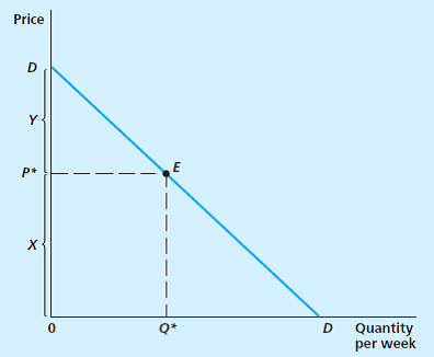
a. With this demand function, what is the value of P for which Q = 0?
b. Use your results from part a together with the fact that distance X in the figure is given by the current price, P*, to show that distance Y is given by -Q*/b (remember, P* is negative here, so this really is a positive distance).
c. To make further progress on this problem, we need to prove Equation 3.13 in the text. To do so, write the definition of price elasticity as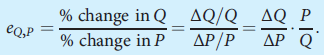
Now use the fact that the demand curve is linear to prove Equation 3.13.
d. Use the result from part c to show that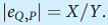 We use the absolute value of the price elasticity here because that elasticity is negative, but the distances X and Y are positive.
e. Explain how the result of part d can be used to demonstrate how the price of elasticity of demand changes as one moves along a linear demand curve.
f. Explain how the results of part c might be used to approximate the price elasticity of demand at any point on a nonlinear demand curve.