Deck 2: Analytics on Spreadsheets
Full screen (f)
Question
Question
Question
Question
Question
Question
Question
Question
Question
Question
Question
Question
Question
Question
Question
Question
Question
Which of the following symbols is used to represent exponents in Excel? 
Question
Question
Question
Question
Question
Question
Question
Question
Question
Question
Question
Question
Question
Question
Question
Identify the equation for calculating the net present value for a stated period of time, where Ft = cash flow in period t, and i is the discount rate. 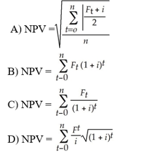
Question
Question
Question
Question
Question
Use the following scenario to answer the following question(s)
The Blue Sunset Band is planning to record a new album. A major decision to be made is if the band can record the album on their own, or if they should hire a studio to record it with. The
fixed cost for recording at the studio is $100,000 plus the manufacturing cost per CD, which is at
$250. If they record the album in-house, the cost per CD is $350. They plan to produce 3000 copies of the album regardless of the place of recording. The band plans to record with the cheaper option. Below is the spreadsheet of the Recording Decision.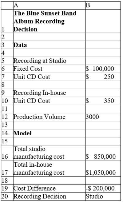
Using the spreadsheet below, provide the steps in using Excel formulas in finding the cost of the first order for Item number 1345, and the total cost of all Item numbers 1345, using the
Match and Index functions in Excel. Column B is sorted by item number in ascending order.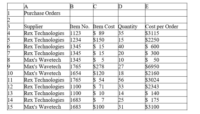
Question
Question
Question

Unlock Deck
Sign up to unlock the cards in this deck!
Unlock Deck
Unlock Deck
1/40
Play
Full screen (f)
Deck 2: Analytics on Spreadsheets
1
For which of the following columns can the COUNT function be performed?
A) column G
B) column E
C) column B
D) column A
A) column G
B) column E
C) column B
D) column A
B
2
To copy a formula from a single cell or range of cells down a column or across a row, first , click and hold the mouse on the small square in the lower right-hand corner of the cell, and drag the formula to the "target" cells which you wish to copy.
A) press Ctrl-C
B) select the cell or range
C) press Ctrl-Enter
D) select the whole spreadsheet
A) press Ctrl-C
B) select the cell or range
C) press Ctrl-Enter
D) select the whole spreadsheet
B
3
Use the data given below to answer the following question(s)
Below is the spreadsheet for demand prediction of a company that sells chocolates.
-If a dollar sign is used before the column label B4 ($B4), how will the formula at B10 be represented in C11 using absolute addressing?
A) $B5-C6*B11
B) $C5-C6*A10
C) $B4-C5*B11
D) $A5-C6*B11
Below is the spreadsheet for demand prediction of a company that sells chocolates.
-If a dollar sign is used before the column label B4 ($B4), how will the formula at B10 be represented in C11 using absolute addressing?
A) $B5-C6*B11
B) $C5-C6*A10
C) $B4-C5*B11
D) $A5-C6*B11
$B5-C6*B11
4
Which of the following ways would 102 × 53 / 100 - 73 be represented in an Excel spreadsheet?
A) 10(2) * 5(3) / 100 ^ 73
B) 10(2) ^ 5(3) / 100 - 73
C) 10^2 * 5^3 / 100 - 73
D) 10*2 ^ 5*3 / 100 - 73
A) 10(2) * 5(3) / 100 ^ 73
B) 10(2) ^ 5(3) / 100 - 73
C) 10^2 * 5^3 / 100 - 73
D) 10*2 ^ 5*3 / 100 - 73
Unlock Deck
Unlock for access to all 40 flashcards in this deck.
Unlock Deck
k this deck
5
Use the data given below to answer the following question(s).
Below is a spreadsheet of purchase orders for a computer hardware retailer.
-To find the largest quantity of items ordered from Rex Technologies, what Excel formula should be used in A12?
A) =COUNTIF(D4:D10)
B) =SUM(D4:D7)
C) =MAX(D4:D7)
D) =COUNT(D4:D7)
Below is a spreadsheet of purchase orders for a computer hardware retailer.
-To find the largest quantity of items ordered from Rex Technologies, what Excel formula should be used in A12?
A) =COUNTIF(D4:D10)
B) =SUM(D4:D7)
C) =MAX(D4:D7)
D) =COUNT(D4:D7)
Unlock Deck
Unlock for access to all 40 flashcards in this deck.
Unlock Deck
k this deck
6
To find the number of orders with A/P terms less than 25 months, what Excel formula should be used in A12?
A) =COUNTIF(F4:F10,"<25")
B) =COUNT(F4:F10,25)
C) =AVERAGE(F4:F10,"<25")
D) =COUNTIF(F4:F10,F5)
A) =COUNTIF(F4:F10,"<25")
B) =COUNT(F4:F10,25)
C) =AVERAGE(F4:F10,"<25")
D) =COUNTIF(F4:F10,F5)
Unlock Deck
Unlock for access to all 40 flashcards in this deck.
Unlock Deck
k this deck
7
Use the data given below to answer the following question(s)
Below is the spreadsheet for demand prediction of a company that sells chocolates.
-Given that D = a-bP, where D, is demand, "a" and "b," are linear constants, and P, is price, from the below spreadsheet, how will the formula in B9 be represented in Excel using relative addressing?
A) B4-B5*A9
B) C5-C6*A10
C) B4-B5*A10
D) B5-B6*A10
Unlock Deck
Unlock for access to all 40 flashcards in this deck.
Unlock Deck
k this deck
8
The reflects the opportunity costs of spending funds now versus achieving a return through another investment, as well as the risks associated with not receiving returns until a later time.
A) modified internal rate of return
B) payback period
C) accounting rate of return
D) discount rate
A) modified internal rate of return
B) payback period
C) accounting rate of return
D) discount rate
Unlock Deck
Unlock for access to all 40 flashcards in this deck.
Unlock Deck
k this deck
9
Use the data given below to answer the following question(s).
Below is a spreadsheet of purchase orders for a computer hardware retailer.
-To find the total order cost, what Excel formula should be used in A12?
A) =COUNT(C4:C10)
B) =COUNT(C4:C7)
C) =MAX(C4:C10)
D) =SUM(E4:E10)
Below is a spreadsheet of purchase orders for a computer hardware retailer.
-To find the total order cost, what Excel formula should be used in A12?
A) =COUNT(C4:C10)
B) =COUNT(C4:C7)
C) =MAX(C4:C10)
D) =SUM(E4:E10)
Unlock Deck
Unlock for access to all 40 flashcards in this deck.
Unlock Deck
k this deck
10
Use the data given below to answer the following question(s)
Below is the spreadsheet for demand prediction of a company that sells chocolates.
-If a dollar sign is used after the column in B5 (B$5), how will the formula at B8 be represented in C9 using absolute addressing?
A) C3-B$5*C9
B) C5-C$6*B9
C) C5-C$6*C9
D) C5-C$5*B9
Below is the spreadsheet for demand prediction of a company that sells chocolates.
-If a dollar sign is used after the column in B5 (B$5), how will the formula at B8 be represented in C9 using absolute addressing?
A) C3-B$5*C9
B) C5-C$6*B9
C) C5-C$6*C9
D) C5-C$5*B9
Unlock Deck
Unlock for access to all 40 flashcards in this deck.
Unlock Deck
k this deck
11
If, in the spreadsheet, cells B9 and B10 were empty, which of the following formulas should be entered in B8 so that the formula can be dragged to B9 and B10 to obtain their correct values?
A) B4-B5*A8
B) B4-B5*$A8
C) $B4-B5*$A8
D) $B$4-$B$5*$A8
A) B4-B5*A8
B) B4-B5*$A8
C) $B4-B5*$A8
D) $B$4-$B$5*$A8
Unlock Deck
Unlock for access to all 40 flashcards in this deck.
Unlock Deck
k this deck
12
Which of the following is a differentiation between calculating using the functions COUNT and COUNTIF?
A) COUNT does not require a range of cells; COUNTIF requires a range of cells.
B) COUNT only requires a range of cell and can be obtained without a special criteria, COUNTIF requires range and special criteria to be calculated.
C) COUNT requires a range of cells; COUNTIF does not require a range of cells, only special criteria.
D) COUNT calculates the sum of values for a range of cells; COUNTIF finds the largest value in a range of cells.
Unlock Deck
Unlock for access to all 40 flashcards in this deck.
Unlock Deck
k this deck
13
Using a $ sign before a column label .
A) keeps the reference to both the row and column fixed
B) keeps the reference to the row fixed, but allows the column reference to change
C) keeps the reference to column fixed, but allows the row reference to change
D) allows both the row and column references to change
A) keeps the reference to both the row and column fixed
B) keeps the reference to the row fixed, but allows the column reference to change
C) keeps the reference to column fixed, but allows the row reference to change
D) allows both the row and column references to change
Unlock Deck
Unlock for access to all 40 flashcards in this deck.
Unlock Deck
k this deck
14
The Excel function of is used to find the largest value in a range of cells.
A) SUM(range)
B) COUNT(range)
C) MAX(range)
D) COUNTIF(range, criteria)
A) SUM(range)
B) COUNT(range)
C) MAX(range)
D) COUNTIF(range, criteria)
Unlock Deck
Unlock for access to all 40 flashcards in this deck.
Unlock Deck
k this deck
15
To find the average of the total cost of orders from Rex Technologies, what Excel formula should be used in A12?
A) =AVERAGE(C4:C10)
B) =AVERAGE(C4:C7)
C) =AVERAGE(E4:E7)
D) =AVERAGE(E4:E10)
A) =AVERAGE(C4:C10)
B) =AVERAGE(C4:C7)
C) =AVERAGE(E4:E7)
D) =AVERAGE(E4:E10)
Unlock Deck
Unlock for access to all 40 flashcards in this deck.
Unlock Deck
k this deck
16
Which of the following is a difference between relative addressing and absolute addressing when using cell formulas in Excel?
A) A relative address uses a dollar sign before either the row or column label; an absolute address uses the ampersand symbol before either the row or column label.
B) A relative address uses a dollar sign before either the row or column label; an absolute address uses just the row and column label in the cell reference.
C) A relative address uses just the row and column label in the cell reference; an absolute address uses a dollar sign before either the row or column label.
D) A relative address uses only the column label in the cell reference; an absolute address uses the row.
Unlock Deck
Unlock for access to all 40 flashcards in this deck.
Unlock Deck
k this deck
17
Which of the following symbols is used to represent exponents in Excel?
Unlock Deck
Unlock for access to all 40 flashcards in this deck.
Unlock Deck
k this deck
18
If purchase quantities of 25 units or higher are found to be large orders, and orders less than 25 are considered to be small, what IF function should be entered in H4 to be copied to H5:H10 to calculate each order's size?
A) =IF(D4=AND=OR=25,"Large","Small")
B) =IF(D4<>25,"Small")=AND(D4=25,"Large")
C) =IF(D4=25,"Large")=OR("Small")
D) =IF(D4>=25,"Large","Small")
A) =IF(D4=AND=OR=25,"Large","Small")
B) =IF(D4<>25,"Small")=AND(D4=25,"Large")
C) =IF(D4=25,"Large")=OR("Small")
D) =IF(D4>=25,"Large","Small")
Unlock Deck
Unlock for access to all 40 flashcards in this deck.
Unlock Deck
k this deck
19
Trace the process of copying and pasting a cell, which has a formula in it, such that the formula is not retained in the pasted cell.
A) Home - Paste - Paste Special - Paste Values
B) Home - Paste - Paste Special - Paste Validation
C) Home - Paste - Paste Special - Paste Formats
D) Home - Paste - Paste Special - Paste Formulas
A) Home - Paste - Paste Special - Paste Values
B) Home - Paste - Paste Special - Paste Validation
C) Home - Paste - Paste Special - Paste Formats
D) Home - Paste - Paste Special - Paste Formulas
Unlock Deck
Unlock for access to all 40 flashcards in this deck.
Unlock Deck
k this deck
20
measures the worth of a stream of cash flows, taking into account the time value of money.
A) Accounting rate of return
B) Net present value
C) Internal rate of return
D) Adjusted present value
A) Accounting rate of return
B) Net present value
C) Internal rate of return
D) Adjusted present value
Unlock Deck
Unlock for access to all 40 flashcards in this deck.
Unlock Deck
k this deck
21
What is the Insert function in Excel?
Unlock Deck
Unlock for access to all 40 flashcards in this deck.
Unlock Deck
k this deck
22
AND(condition 1, condition 2…) is a logical function that returns TRUE if all conditions are true and FALSE if not.
Unlock Deck
Unlock for access to all 40 flashcards in this deck.
Unlock Deck
k this deck
23
is a logical function that returns one value if the condition is true and another if the condition is false.
A) OR(condition 1, condition 2…)
B) AND(condition 1, condition 2…)
C) TO(value if true, value if false)
D) IF(condition, value if true, value if false)
A) OR(condition 1, condition 2…)
B) AND(condition 1, condition 2…)
C) TO(value if true, value if false)
D) IF(condition, value if true, value if false)
Unlock Deck
Unlock for access to all 40 flashcards in this deck.
Unlock Deck
k this deck
24
In a MATCH function, if match_type = 1, then the function finds the smallest value that is greater than or equal to lookup_value.
Unlock Deck
Unlock for access to all 40 flashcards in this deck.
Unlock Deck
k this deck
25
Describe the method of calculating the net present value (NPV) in Excel.
Unlock Deck
Unlock for access to all 40 flashcards in this deck.
Unlock Deck
k this deck
26
The function returns a value or reference of the cell at the intersection of a particular row and column in a given range.
A) VLOOKUP(lookup_value, table_array, col_index_num)
B) INDEX(array, row_num, col_num)
C) MATCH(lookup_value, lookup_array, match_type)
D) HLOOKUP(lookup_value, table_array, row_index_num)
A) VLOOKUP(lookup_value, table_array, col_index_num)
B) INDEX(array, row_num, col_num)
C) MATCH(lookup_value, lookup_array, match_type)
D) HLOOKUP(lookup_value, table_array, row_index_num)
Unlock Deck
Unlock for access to all 40 flashcards in this deck.
Unlock Deck
k this deck
27
To use the VLOOKUP(lookup_value, table_array, col_index_num), the table must be sorted in descending order.
Unlock Deck
Unlock for access to all 40 flashcards in this deck.
Unlock Deck
k this deck
28
If cell G7 contains the function , it states that if the value in cell C3 is 9, the number 7 will be assigned to cell G7; if the value in cell C3 is not 9, the number 4 will be assigned to cell G7.
A) =IF(G7=9)(G7=7)=OR(G7=4)
B) =IF(G7=7)=THEN(C3=9)=OR(C3=4)
C) =IF(C3=9)(C3=7)=OR(C3=4)
D) =IF(C3=9,7,4)
A) =IF(G7=9)(G7=7)=OR(G7=4)
B) =IF(G7=7)=THEN(C3=9)=OR(C3=4)
C) =IF(C3=9)(C3=7)=OR(C3=4)
D) =IF(C3=9,7,4)
Unlock Deck
Unlock for access to all 40 flashcards in this deck.
Unlock Deck
k this deck
29
Using a $ sign before both the row and column labels keeps the reference to that cell fixed no matter where the formula is copied.
Unlock Deck
Unlock for access to all 40 flashcards in this deck.
Unlock Deck
k this deck
30
A positive NPV means that the investment will provide added value because the projected return exceeds the .
A) modified internal rate of return
B) discount rate
C) accounting rate of return
D) adjusted present value
A) modified internal rate of return
B) discount rate
C) accounting rate of return
D) adjusted present value
Unlock Deck
Unlock for access to all 40 flashcards in this deck.
Unlock Deck
k this deck
31
The easiest way to locate a particular function is to select a cell and click on the Insert function button represented by on the Excel ribbon.
A) fx
B) Σ
C) $
D) %
A) fx
B) Σ
C) $
D) %
Unlock Deck
Unlock for access to all 40 flashcards in this deck.
Unlock Deck
k this deck
32
Identify the equation for calculating the net present value for a stated period of time, where Ft = cash flow in period t, and i is the discount rate.
Unlock Deck
Unlock for access to all 40 flashcards in this deck.
Unlock Deck
k this deck
33
For which of the following MATCH functions must the values in the lookup_array be ordered in a descending order?
A) When match_type = -1
B) When match_type >1
C) When match_type = 0
D) When match_type = 1
A) When match_type = -1
B) When match_type >1
C) When match_type = 0
D) When match_type = 1
Unlock Deck
Unlock for access to all 40 flashcards in this deck.
Unlock Deck
k this deck
34
Explain the different Lookup functions in Excel.
Unlock Deck
Unlock for access to all 40 flashcards in this deck.
Unlock Deck
k this deck
35
In a MATCH function, if the match_type = 0, then .
A) the function finds the largest value that is less than or equal to lookup_value
B) the function finds the smallest value that is greater than or equal to lookup_value
C) MATCH finds the first value that is exactly equal to lookup_value
D) the values in the lookup_array must be in a particular order
Unlock Deck
Unlock for access to all 40 flashcards in this deck.
Unlock Deck
k this deck
36
In a MATCH function, the default value for match_type = 0.
Unlock Deck
Unlock for access to all 40 flashcards in this deck.
Unlock Deck
k this deck
37
Use the following scenario to answer the following question(s)
The Blue Sunset Band is planning to record a new album. A major decision to be made is if the band can record the album on their own, or if they should hire a studio to record it with. The
fixed cost for recording at the studio is $100,000 plus the manufacturing cost per CD, which is at
$250. If they record the album in-house, the cost per CD is $350. They plan to produce 3000 copies of the album regardless of the place of recording. The band plans to record with the cheaper option. Below is the spreadsheet of the Recording Decision.
Using the spreadsheet below, provide the steps in using Excel formulas in finding the cost of the first order for Item number 1345, and the total cost of all Item numbers 1345, using the
Match and Index functions in Excel. Column B is sorted by item number in ascending order.
The Blue Sunset Band is planning to record a new album. A major decision to be made is if the band can record the album on their own, or if they should hire a studio to record it with. The
fixed cost for recording at the studio is $100,000 plus the manufacturing cost per CD, which is at
$250. If they record the album in-house, the cost per CD is $350. They plan to produce 3000 copies of the album regardless of the place of recording. The band plans to record with the cheaper option. Below is the spreadsheet of the Recording Decision.
Using the spreadsheet below, provide the steps in using Excel formulas in finding the cost of the first order for Item number 1345, and the total cost of all Item numbers 1345, using the
Match and Index functions in Excel. Column B is sorted by item number in ascending order.
Unlock Deck
Unlock for access to all 40 flashcards in this deck.
Unlock Deck
k this deck
38
Give the logical function for the following: If cell B7 equals 12, check contents of cell B10. If cell B10 is 10, then the value of the function in the string is YES; if not, it is a blank space. If cell B7 does not equal 12, then the value of the function is 7.
A) =IF(B7=12,(AND(B10=10, "")(YES)),7)
B) =IF(B10=10,(OR(B7=12,"")"YES")7)
C) =IF(B7=12,(IF(B10=10,"YES", "")),7)
D) =IF(B7=12,(AND(B10=10,"YES","")(B10="NO"),7)
A) =IF(B7=12,(AND(B10=10, "")(YES)),7)
B) =IF(B10=10,(OR(B7=12,"")"YES")7)
C) =IF(B7=12,(IF(B10=10,"YES", "")),7)
D) =IF(B7=12,(AND(B10=10,"YES","")(B10="NO"),7)
Unlock Deck
Unlock for access to all 40 flashcards in this deck.
Unlock Deck
k this deck
39
Which of the following functions is a logical function that returns TRUE if any condition is true and FALSE if not?
A) TO(value if true, value if false)
B) AND(condition 1, condition 2…)
C) OR(condition 1, condition 2…)
D) IF(condition, value if true, value if false)
A) TO(value if true, value if false)
B) AND(condition 1, condition 2…)
C) OR(condition 1, condition 2…)
D) IF(condition, value if true, value if false)
Unlock Deck
Unlock for access to all 40 flashcards in this deck.
Unlock Deck
k this deck
40
Which of the following Lookup functions returns the relative position of an item in an array that equals a specified value in a specified order?
A) HLOOKUP(lookup_value, table_array, row_index_num)
B) MATCH(lookup_value, lookup_array, match_type)
C) INDEX(array, row_num, col_num)
D) VLOOKUP(lookup_value, table_array, col_index_num)
A) HLOOKUP(lookup_value, table_array, row_index_num)
B) MATCH(lookup_value, lookup_array, match_type)
C) INDEX(array, row_num, col_num)
D) VLOOKUP(lookup_value, table_array, col_index_num)
Unlock Deck
Unlock for access to all 40 flashcards in this deck.
Unlock Deck
k this deck
Unlock Deck
Unlock for access to all 40 flashcards in this deck.


