Deck 2: Review of Probability
Full screen (f)
Question
Question
Question
Question
Question
Two random variables X and Y are independently distributed if all of the following conditions hold, with the exception of 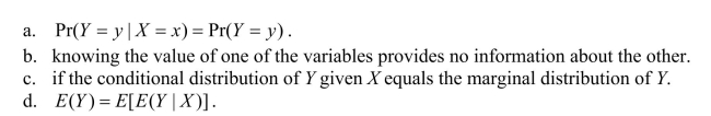
Question
Question
Question
Let Y be a random variable.Then var(Y)equals 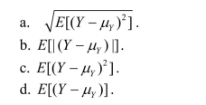
Question
Question
The kurtosis of a distribution is defined as follows: 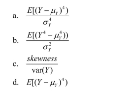
Question
Question
Question
Question
Two variables are uncorrelated in all of the cases below, with the exception of 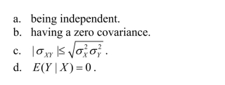
Question
The skewness of the distribution of a random variable Y is defined as follows: 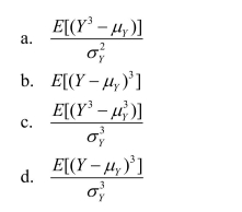
Question
Question
Question
The correlation between X and Y 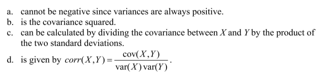
Question
Question
If variables with a multivariate normal distribution have covariances that equal zero, then 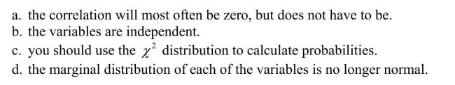
Question
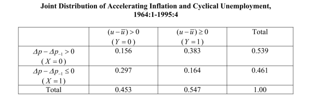
The expectations augmented Phillips curve postulates 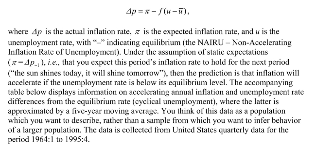
 (a)Compute EY( )and EX( ), and interpret both numbers.
(a)Compute EY( )and EX( ), and interpret both numbers. Question
Probabilities and relative frequencies are related in that the probability of an outcome is
the proportion of the time that the outcome occurs in the long run.Hence concepts of
joint, marginal, and conditional probability distributions stem from related concepts of
frequency distributions.
You are interested in investigating the relationship between the age of heads of
households and weekly earnings of households.The accompanying data gives the number
of occurrences grouped by age and income.You collect data from 1,744 individuals and
think of these individuals as a population that you want to describe, rather than a sample
from which you want to infer behavior of a larger population.After sorting the data, you
generate the accompanying table: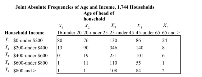 The median of the income group of $800 and above is $1,050.
(a)Calculate the joint relative frequencies and the marginal relative frequencies.Interpret
one of each of these.Sketch the cumulative income distribution.
the proportion of the time that the outcome occurs in the long run.Hence concepts of
joint, marginal, and conditional probability distributions stem from related concepts of
frequency distributions.
You are interested in investigating the relationship between the age of heads of
households and weekly earnings of households.The accompanying data gives the number
of occurrences grouped by age and income.You collect data from 1,744 individuals and
think of these individuals as a population that you want to describe, rather than a sample
from which you want to infer behavior of a larger population.After sorting the data, you
generate the accompanying table:
The median of the income group of $800 and above is $1,050.(a)Calculate the joint relative frequencies and the marginal relative frequencies.Interpret
one of each of these.Sketch the cumulative income distribution.
Question
You have read about the so-called catch-up theory by economic historians, whereby nations
that are further behind in per capita income grow faster subsequently.If this is true
systematically, then eventually laggards will reach the leader.To put the theory to the test,
you collect data on relative (to the United States)per capita income for two years, 1960 and
1990, for 24 OECD countries.You think of these countries as a population you want to
describe, rather than a sample from which you want to infer behavior of a larger population.
The relevant data for this question is as follows: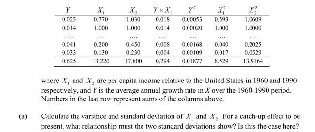
Question
A few years ago the news magazine The Economist listed some of the stranger
explanations used in the past to predict presidential election outcomes.These included
whether or not the hemlines of women's skirts went up or down, stock market
performances, baseball World Series wins by an American League team, etc.Thinking
about this problem more seriously, you decide to analyze whether or not the presidential
candidate for a certain party did better if his party controlled the house.Accordingly you
collect data for the last 34 presidential elections.You think of this data as comprising a
population which you want to describe, rather than a sample from which you want to
infer behavior of a larger population.You generate the accompanying table: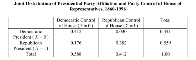 (a)Interpret one of the joint probabilities and one of the marginal probabilities.
explanations used in the past to predict presidential election outcomes.These included
whether or not the hemlines of women's skirts went up or down, stock market
performances, baseball World Series wins by an American League team, etc.Thinking
about this problem more seriously, you decide to analyze whether or not the presidential
candidate for a certain party did better if his party controlled the house.Accordingly you
collect data for the last 34 presidential elections.You think of this data as comprising a
population which you want to describe, rather than a sample from which you want to
infer behavior of a larger population.You generate the accompanying table:
(a)Interpret one of the joint probabilities and one of the marginal probabilities. Question
The sample average is a random variable and 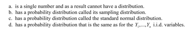
Question
Question
What is the probability of the following outcomes? 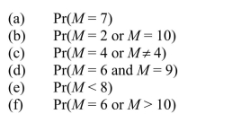
Question
The table accompanying lists the joint distribution of unemployment in the United States
in 2001 by demographic characteristics (race and gender).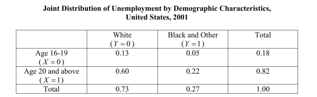 (a)What is the percentage of unemployed white teenagers?
in 2001 by demographic characteristics (race and gender).
(a)What is the percentage of unemployed white teenagers? Question
Question
In econometrics, we typically do not rely on exact or finite sample distributions because 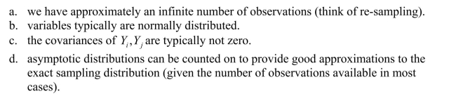
Question
Question
Question
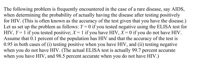 (a)Assuming arbitrarily a population of 10,000,000 people, use the accompanying table to
first enter the column totals.
Question
Question
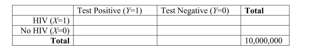
The accompanying table shows the joint distribution between the change of the
unemployment rate in an election year and the share of the candidate of the incumbent
party since 1928.You think of this data as a population which you want to describe,
rather than a sample from which you want to infer behavior of a larger population. (a)Compute and interpret E()Y and E()X .
unemployment rate in an election year and the share of the candidate of the incumbent
party since 1928.You think of this data as a population which you want to describe,
rather than a sample from which you want to infer behavior of a larger population.
(a)Compute and interpret E()Y and E()X . Question
The central limit theorem states that 
Question
The covariance inequality states that 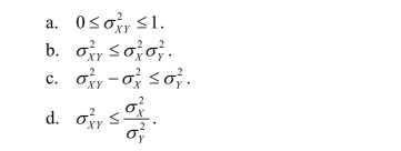
Question
Question
Following Alfred Nobel's will, there are five Nobel Prizes awarded each year.These are
for outstanding achievements in Chemistry, Physics, Physiology or Medicine, Literature,
and Peace.In 1968, the Bank of Sweden added a prize in Economic Sciences in memory
of Alfred Nobel.You think of the data as describing a population, rather than a sample
from which you want to infer behavior of a larger population.The accompanying table
lists the joint probability distribution between recipients in economics and the other five
prizes, and the citizenship of the recipients, based on the 1969-2001 period.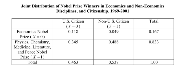 (a)Compute EY( )and interpret the resulting number.
for outstanding achievements in Chemistry, Physics, Physiology or Medicine, Literature,
and Peace.In 1968, the Bank of Sweden added a prize in Economic Sciences in memory
of Alfred Nobel.You think of the data as describing a population, rather than a sample
from which you want to infer behavior of a larger population.The accompanying table
lists the joint probability distribution between recipients in economics and the other five
prizes, and the citizenship of the recipients, based on the 1969-2001 period.
(a)Compute EY( )and interpret the resulting number. Question
The central limit theorem 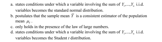
Question
The accompanying table lists the outcomes and the cumulative probability distribution
for a student renting videos during the week while on campus.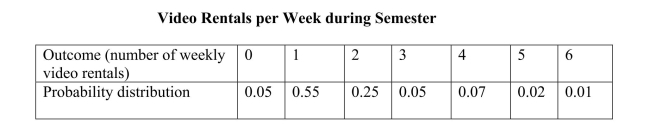 Sketch the probability distribution.Next, calculate the cumulative probability
distribution for the above table.What is the probability of the student renting between 2
and 4 a week? Of less than 3 a week?
for a student renting videos during the week while on campus.
Sketch the probability distribution.Next, calculate the cumulative probabilitydistribution for the above table.What is the probability of the student renting between 2
and 4 a week? Of less than 3 a week?
Question
There are frequently situations where you have information on the conditional distribution of Y given X , but are interested in the conditional distribution of X given Y .
Recalling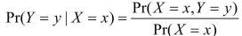
, derive a relationship between

This is called Bayes' theorem.
Recalling
, derive a relationship between
This is called Bayes' theorem.
Question
You are at a college of roughly 1,000 students and obtain data from the entire freshman
class (250 students)on height and weight during orientation.You consider this to be a
population that you want to describe, rather than a sample from which you want to infer
general relationships in a larger population.Weight (Y)is measured in pounds and height
(X)is measured in inches.You calculate the following sums: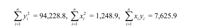
 (a)Given your general knowledge about human height and weight of a given age, what can
you say about the shape of the two distributions?
class (250 students)on height and weight during orientation.You consider this to be a
population that you want to describe, rather than a sample from which you want to infer
general relationships in a larger population.Weight (Y)is measured in pounds and height
(X)is measured in inches.You calculate the following sums:
(a)Given your general knowledge about human height and weight of a given age, what canyou say about the shape of the two distributions?
Question
The textbook mentioned that the mean of Y, E(Y) is called the first moment of Y , and that the expected value of the square of  is called the second moment of Y , and so on. These are also referred to as moments about the origin. A related concept is moments about the mean, which are defined as
What do you call the second moment about the mean? What do you think the third moment, referred to as "skewness," measures? Do you believe that it would be positive or negative for an earnings distribution? What measure of the third moment around the mean do you get for a normal distribution?
is called the second moment of Y , and so on. These are also referred to as moments about the origin. A related concept is moments about the mean, which are defined as What do you call the second moment about the mean? What do you think the third moment, referred to as "skewness," measures? Do you believe that it would be positive or negative for an earnings distribution? What measure of the third moment around the mean do you get for a normal distribution?
Question
Question
Question
The textbook formula for the variance of the discrete random variable Y is given as 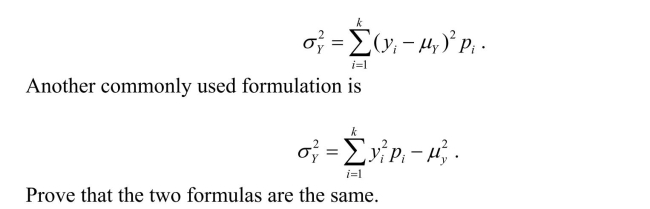
Question
Question
The Economic Report of the President gives the following age distribution of the United
States population for the year 2000: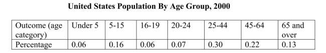 Imagine that every person was assigned a unique number between 1 and 275,372,000 (the
total population in 2000).If you generated a random number, what would be the
probability that you had drawn someone older than 65 or under 16? Treating the
percentages as probabilities, write down the cumulative probability distribution.What is
the probability of drawing someone who is 24 years or younger?
States population for the year 2000:
Imagine that every person was assigned a unique number between 1 and 275,372,000 (thetotal population in 2000).If you generated a random number, what would be the
probability that you had drawn someone older than 65 or under 16? Treating the
percentages as probabilities, write down the cumulative probability distribution.What is
the probability of drawing someone who is 24 years or younger?
Question
Question
Calculate the following probabilities using the standard normal distribution.Sketch the
probability distribution in each case, shading in the area of the calculated probability.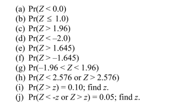
probability distribution in each case, shading in the area of the calculated probability.
Question
Question
Show that the correlation coefficient between Y and X is unaffected if you use a linear transformation in both variables. That is, show that 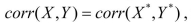 where
where 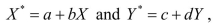 and where a, b, c , and d are arbitrary non-zero constants.
where and where a, b, c , and d are arbitrary non-zero constants. Question
In considering the purchase of a certain stock, you attach the following probabilities to
possible changes in the stock price over the next year. What is the expected value, the variance, and the standard deviation? Which is the most
likely outcome? Sketch the cumulative distribution function.
.
possible changes in the stock price over the next year.
What is the expected value, the variance, and the standard deviation? Which is the mostlikely outcome? Sketch the cumulative distribution function.
.
Question
The accompanying table gives the outcomes and probability distribution of the number of
times a student checks her e-mail daily: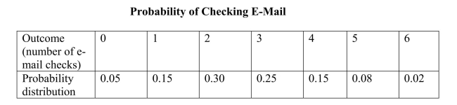 Sketch the probability distribution.Next, calculate the c.d.f.for the above table.What is
the probability of her checking her e-mail between 1 and 3 times a day? Of checking it
more than 3 times a day?
times a student checks her e-mail daily:
Sketch the probability distribution.Next, calculate the c.d.f.for the above table.What isthe probability of her checking her e-mail between 1 and 3 times a day? Of checking it
more than 3 times a day?
Question
You consider visiting Montreal during the break between terms in January.You go to the
relevant Web site of the official tourist office to figure out the type of clothes you should
take on the trip.The site lists that the average high during January is -70 C, with a
standard deviation of 40 C.Unfortunately you are more familiar with Fahrenheit than
with Celsius, but find that the two are related by the following linear function: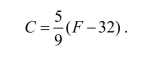 Find the mean and standard deviation for the January temperature in Montreal in
Fahrenheit.
relevant Web site of the official tourist office to figure out the type of clothes you should
take on the trip.The site lists that the average high during January is -70 C, with a
standard deviation of 40 C.Unfortunately you are more familiar with Fahrenheit than
with Celsius, but find that the two are related by the following linear function:
Find the mean and standard deviation for the January temperature in Montreal inFahrenheit.
Question
Find the following probabilities:
(a)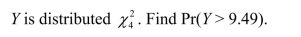
(a)
Question
Question
Question
What would the correlation coefficient be if all observations for the two variables were
on a curve described by
on a curve described by
Question
Explain why the two probabilities are identical for the standard normal distribution:


Unlock Deck
Sign up to unlock the cards in this deck!
Unlock Deck
Unlock Deck
1/61
Play
Full screen (f)
Deck 2: Review of Probability
1
Assume that Y is normally distributed To find where and , you need to calculate
A)
B)
C)
D)
A)
B)
C)
D)
2
A)
B)
C)
D)
3
When there are degrees of freedom, the distribution
A) can no longer be calculated.
B) equals the standard normal distribution.
C) has a bell shape similar to that of the normal distribution, but with "fatter" tails.
D) equals the distribution.
A) can no longer be calculated.
B) equals the standard normal distribution.
C) has a bell shape similar to that of the normal distribution, but with "fatter" tails.
D) equals the distribution.
equals the standard normal distribution.
4
The probability of an event
to occur equals
A)
B)
C)
D)
to occur equals
A)
B)
C)
D)
Unlock Deck
Unlock for access to all 61 flashcards in this deck.
Unlock Deck
k this deck
5
Two random variables X and Y are independently distributed if all of the following conditions hold, with the exception of
Unlock Deck
Unlock for access to all 61 flashcards in this deck.
Unlock Deck
k this deck
6
The cumulative probability distribution shows the probability
A)that a random variable is less than or equal to a particular value.
B)of two or more events occurring at once.
C)of all possible events occurring.
D)that a random variable takes on a particular value given that another event has happened.
A)that a random variable is less than or equal to a particular value.
B)of two or more events occurring at once.
C)of all possible events occurring.
D)that a random variable takes on a particular value given that another event has happened.
Unlock Deck
Unlock for access to all 61 flashcards in this deck.
Unlock Deck
k this deck
7
The skewness is most likely positive for one of the following distributions:
A)The grade distribution at your college or university.
B)The U.S.income distribution.
C)SAT scores in English.
D)The height of 18-year-old females in the U.S.
A)The grade distribution at your college or university.
B)The U.S.income distribution.
C)SAT scores in English.
D)The height of 18-year-old females in the U.S.
Unlock Deck
Unlock for access to all 61 flashcards in this deck.
Unlock Deck
k this deck
8
Let Y be a random variable.Then var(Y)equals
Unlock Deck
Unlock for access to all 61 flashcards in this deck.
Unlock Deck
k this deck
9
Assume that Y is normally distributed
Moving from the mean 1.96 standard deviations to the left and 1.96 standard deviations to the right, then the area under the normal p.d.f. is
A) 0.67
B) 0.05
C) 0.95
D) 0.33
Moving from the mean 1.96 standard deviations to the left and 1.96 standard deviations to the right, then the area under the normal p.d.f. is
A) 0.67
B) 0.05
C) 0.95
D) 0.33
Unlock Deck
Unlock for access to all 61 flashcards in this deck.
Unlock Deck
k this deck
10
The kurtosis of a distribution is defined as follows:
Unlock Deck
Unlock for access to all 61 flashcards in this deck.
Unlock Deck
k this deck
11
The conditional expectation of Y given
is calculated as follows:
A)
B)
C)
D)
is calculated as follows:
A)
B)
C)
D)
Unlock Deck
Unlock for access to all 61 flashcards in this deck.
Unlock Deck
k this deck
12
The Student t distribution is
A)the distribution of the sum of m squared independent standard normal random variables.
B)the distribution of a random variable with a chi-squared distribution with m degrees of freedom, divided by m.
C)always well approximated by the standard normal distribution.
D)the distribution of the ratio of a standard normal random variable, divided by the square root of an independently distributed chi-squared random variable with m
Degrees of freedom divided by m.
Unlock Deck
Unlock for access to all 61 flashcards in this deck.
Unlock Deck
k this deck
13
The conditional distribution of Y given
is
A)
B)
C)
D)
is
A)
B)
C)
D)
Unlock Deck
Unlock for access to all 61 flashcards in this deck.
Unlock Deck
k this deck
14
Two variables are uncorrelated in all of the cases below, with the exception of
Unlock Deck
Unlock for access to all 61 flashcards in this deck.
Unlock Deck
k this deck
15
The skewness of the distribution of a random variable Y is defined as follows:
Unlock Deck
Unlock for access to all 61 flashcards in this deck.
Unlock Deck
k this deck
16
To standardize a variable you
A)subtract its mean and divide by its standard deviation.
B)integrate the area below two points under the normal distribution.
C)add and subtract 1.96 times the standard deviation to the variable.
D)divide it by its standard deviation, as long as its mean is 1.
A)subtract its mean and divide by its standard deviation.
B)integrate the area below two points under the normal distribution.
C)add and subtract 1.96 times the standard deviation to the variable.
D)divide it by its standard deviation, as long as its mean is 1.
Unlock Deck
Unlock for access to all 61 flashcards in this deck.
Unlock Deck
k this deck
17
The probability of an outcome
A)is the number of times that the outcome occurs in the long run.
B)equals M× N, where M is the number of occurrences and N is the population size.
C)is the proportion of times that the outcome occurs in the long run.
D)equals the sample mean divided by the sample standard deviation.
A)is the number of times that the outcome occurs in the long run.
B)equals M× N, where M is the number of occurrences and N is the population size.
C)is the proportion of times that the outcome occurs in the long run.
D)equals the sample mean divided by the sample standard deviation.
Unlock Deck
Unlock for access to all 61 flashcards in this deck.
Unlock Deck
k this deck
18
The correlation between X and Y
Unlock Deck
Unlock for access to all 61 flashcards in this deck.
Unlock Deck
k this deck
19
For a normal distribution, the skewness and kurtosis measures are as follows:
A)1.96 and 4
B)0 and 0
C)0 and 3
D)1 and 2
A)1.96 and 4
B)0 and 0
C)0 and 3
D)1 and 2
Unlock Deck
Unlock for access to all 61 flashcards in this deck.
Unlock Deck
k this deck
20
If variables with a multivariate normal distribution have covariances that equal zero, then
Unlock Deck
Unlock for access to all 61 flashcards in this deck.
Unlock Deck
k this deck
21
The expectations augmented Phillips curve postulates (a)Compute EY( )and EX( ), and interpret both numbers.
(a)Compute EY( )and EX( ), and interpret both numbers. Unlock Deck
Unlock for access to all 61 flashcards in this deck.
Unlock Deck
k this deck
22
Probabilities and relative frequencies are related in that the probability of an outcome is
the proportion of the time that the outcome occurs in the long run.Hence concepts of
joint, marginal, and conditional probability distributions stem from related concepts of
frequency distributions.
You are interested in investigating the relationship between the age of heads of
households and weekly earnings of households.The accompanying data gives the number
of occurrences grouped by age and income.You collect data from 1,744 individuals and
think of these individuals as a population that you want to describe, rather than a sample
from which you want to infer behavior of a larger population.After sorting the data, you
generate the accompanying table: The median of the income group of $800 and above is $1,050.
(a)Calculate the joint relative frequencies and the marginal relative frequencies.Interpret
one of each of these.Sketch the cumulative income distribution.
the proportion of the time that the outcome occurs in the long run.Hence concepts of
joint, marginal, and conditional probability distributions stem from related concepts of
frequency distributions.
You are interested in investigating the relationship between the age of heads of
households and weekly earnings of households.The accompanying data gives the number
of occurrences grouped by age and income.You collect data from 1,744 individuals and
think of these individuals as a population that you want to describe, rather than a sample
from which you want to infer behavior of a larger population.After sorting the data, you
generate the accompanying table:
The median of the income group of $800 and above is $1,050.(a)Calculate the joint relative frequencies and the marginal relative frequencies.Interpret
one of each of these.Sketch the cumulative income distribution.
Unlock Deck
Unlock for access to all 61 flashcards in this deck.
Unlock Deck
k this deck
23
You have read about the so-called catch-up theory by economic historians, whereby nations
that are further behind in per capita income grow faster subsequently.If this is true
systematically, then eventually laggards will reach the leader.To put the theory to the test,
you collect data on relative (to the United States)per capita income for two years, 1960 and
1990, for 24 OECD countries.You think of these countries as a population you want to
describe, rather than a sample from which you want to infer behavior of a larger population.
The relevant data for this question is as follows:
that are further behind in per capita income grow faster subsequently.If this is true
systematically, then eventually laggards will reach the leader.To put the theory to the test,
you collect data on relative (to the United States)per capita income for two years, 1960 and
1990, for 24 OECD countries.You think of these countries as a population you want to
describe, rather than a sample from which you want to infer behavior of a larger population.
The relevant data for this question is as follows:
Unlock Deck
Unlock for access to all 61 flashcards in this deck.
Unlock Deck
k this deck
24
A few years ago the news magazine The Economist listed some of the stranger
explanations used in the past to predict presidential election outcomes.These included
whether or not the hemlines of women's skirts went up or down, stock market
performances, baseball World Series wins by an American League team, etc.Thinking
about this problem more seriously, you decide to analyze whether or not the presidential
candidate for a certain party did better if his party controlled the house.Accordingly you
collect data for the last 34 presidential elections.You think of this data as comprising a
population which you want to describe, rather than a sample from which you want to
infer behavior of a larger population.You generate the accompanying table: (a)Interpret one of the joint probabilities and one of the marginal probabilities.
explanations used in the past to predict presidential election outcomes.These included
whether or not the hemlines of women's skirts went up or down, stock market
performances, baseball World Series wins by an American League team, etc.Thinking
about this problem more seriously, you decide to analyze whether or not the presidential
candidate for a certain party did better if his party controlled the house.Accordingly you
collect data for the last 34 presidential elections.You think of this data as comprising a
population which you want to describe, rather than a sample from which you want to
infer behavior of a larger population.You generate the accompanying table:
(a)Interpret one of the joint probabilities and one of the marginal probabilities. Unlock Deck
Unlock for access to all 61 flashcards in this deck.
Unlock Deck
k this deck
25
The sample average is a random variable and
Unlock Deck
Unlock for access to all 61 flashcards in this deck.
Unlock Deck
k this deck
26
To infer the political tendencies of the students at your college/university, you sample 150 of them.Only one of the following is a simple random sample: You
A)make sure that the proportion of minorities are the same in your sample as in the entire student body.
A)m.If the person does not answer the phone, you pick the next name listed, and so on.
B)call every fiftieth person in the student directory at 9
C)go to the main dining hall on campus and interview students randomly there.
D)have your statistical package generate 150 random numbers in the range from 1 to the total number of students in your academic institution, and then choose
The corresponding names in the student telephone directory.
Unlock Deck
Unlock for access to all 61 flashcards in this deck.
Unlock Deck
k this deck
27
What is the probability of the following outcomes?
Unlock Deck
Unlock for access to all 61 flashcards in this deck.
Unlock Deck
k this deck
28
The table accompanying lists the joint distribution of unemployment in the United States
in 2001 by demographic characteristics (race and gender). (a)What is the percentage of unemployed white teenagers?
in 2001 by demographic characteristics (race and gender).
(a)What is the percentage of unemployed white teenagers? Unlock Deck
Unlock for access to all 61 flashcards in this deck.
Unlock Deck
k this deck
29
Math and verbal SAT scores are each distributed normally with N(500,10000).
(a) What fraction of students scores above 750? Above 600? Between 420 and 530? Below
480? Above 530?
(a) What fraction of students scores above 750? Above 600? Between 420 and 530? Below
480? Above 530?
Unlock Deck
Unlock for access to all 61 flashcards in this deck.
Unlock Deck
k this deck
30
In econometrics, we typically do not rely on exact or finite sample distributions because
Unlock Deck
Unlock for access to all 61 flashcards in this deck.
Unlock Deck
k this deck
31
Think of the situation of rolling two dice and let M denote the sum of the number of dots
on the two dice.(So M is a number between 1 and 12.)
(a)In a table, list all of the possible outcomes for the random variable M together with its
probability distribution and cumulative probability distribution.Sketch both distributions.
on the two dice.(So M is a number between 1 and 12.)
(a)In a table, list all of the possible outcomes for the random variable M together with its
probability distribution and cumulative probability distribution.Sketch both distributions.
Unlock Deck
Unlock for access to all 61 flashcards in this deck.
Unlock Deck
k this deck
32
Consistency for the sample average can be defined as follows, with the exception of
A) converges in probability to
B) has the smallest variance of all estimators.
C)
D) the probability of being in the range becomes arbitrarily close to one as increases for any constant c>0 .
A) converges in probability to
B) has the smallest variance of all estimators.
C)
D) the probability of being in the range becomes arbitrarily close to one as increases for any constant c>0 .
Unlock Deck
Unlock for access to all 61 flashcards in this deck.
Unlock Deck
k this deck
33
(a)Assuming arbitrarily a population of 10,000,000 people, use the accompanying table tofirst enter the column totals.
Unlock Deck
Unlock for access to all 61 flashcards in this deck.
Unlock Deck
k this deck
34
The mean of the sample average is
A)
B)
C)
D) for n>30 .
A)
B)
C)
D) for n>30 .
Unlock Deck
Unlock for access to all 61 flashcards in this deck.
Unlock Deck
k this deck
35
The accompanying table shows the joint distribution between the change of the
unemployment rate in an election year and the share of the candidate of the incumbent
party since 1928.You think of this data as a population which you want to describe,
rather than a sample from which you want to infer behavior of a larger population. (a)Compute and interpret E()Y and E()X .
unemployment rate in an election year and the share of the candidate of the incumbent
party since 1928.You think of this data as a population which you want to describe,
rather than a sample from which you want to infer behavior of a larger population.
(a)Compute and interpret E()Y and E()X . Unlock Deck
Unlock for access to all 61 flashcards in this deck.
Unlock Deck
k this deck
36
The central limit theorem states that
Unlock Deck
Unlock for access to all 61 flashcards in this deck.
Unlock Deck
k this deck
37
The covariance inequality states that
Unlock Deck
Unlock for access to all 61 flashcards in this deck.
Unlock Deck
k this deck
38
The variance of is given by the following formula:
A)
B)
C)
D)
A)
B)
C)
D)
Unlock Deck
Unlock for access to all 61 flashcards in this deck.
Unlock Deck
k this deck
39
Following Alfred Nobel's will, there are five Nobel Prizes awarded each year.These are
for outstanding achievements in Chemistry, Physics, Physiology or Medicine, Literature,
and Peace.In 1968, the Bank of Sweden added a prize in Economic Sciences in memory
of Alfred Nobel.You think of the data as describing a population, rather than a sample
from which you want to infer behavior of a larger population.The accompanying table
lists the joint probability distribution between recipients in economics and the other five
prizes, and the citizenship of the recipients, based on the 1969-2001 period. (a)Compute EY( )and interpret the resulting number.
for outstanding achievements in Chemistry, Physics, Physiology or Medicine, Literature,
and Peace.In 1968, the Bank of Sweden added a prize in Economic Sciences in memory
of Alfred Nobel.You think of the data as describing a population, rather than a sample
from which you want to infer behavior of a larger population.The accompanying table
lists the joint probability distribution between recipients in economics and the other five
prizes, and the citizenship of the recipients, based on the 1969-2001 period.
(a)Compute EY( )and interpret the resulting number. Unlock Deck
Unlock for access to all 61 flashcards in this deck.
Unlock Deck
k this deck
40
The central limit theorem
Unlock Deck
Unlock for access to all 61 flashcards in this deck.
Unlock Deck
k this deck
41
The accompanying table lists the outcomes and the cumulative probability distribution
for a student renting videos during the week while on campus. Sketch the probability distribution.Next, calculate the cumulative probability
distribution for the above table.What is the probability of the student renting between 2
and 4 a week? Of less than 3 a week?
for a student renting videos during the week while on campus.
Sketch the probability distribution.Next, calculate the cumulative probabilitydistribution for the above table.What is the probability of the student renting between 2
and 4 a week? Of less than 3 a week?
Unlock Deck
Unlock for access to all 61 flashcards in this deck.
Unlock Deck
k this deck
42
There are frequently situations where you have information on the conditional distribution of Y given X , but are interested in the conditional distribution of X given Y .
Recalling
, derive a relationship between
This is called Bayes' theorem.
Recalling
, derive a relationship between
This is called Bayes' theorem.
Unlock Deck
Unlock for access to all 61 flashcards in this deck.
Unlock Deck
k this deck
43
You are at a college of roughly 1,000 students and obtain data from the entire freshman
class (250 students)on height and weight during orientation.You consider this to be a
population that you want to describe, rather than a sample from which you want to infer
general relationships in a larger population.Weight (Y)is measured in pounds and height
(X)is measured in inches.You calculate the following sums: (a)Given your general knowledge about human height and weight of a given age, what can
you say about the shape of the two distributions?
class (250 students)on height and weight during orientation.You consider this to be a
population that you want to describe, rather than a sample from which you want to infer
general relationships in a larger population.Weight (Y)is measured in pounds and height
(X)is measured in inches.You calculate the following sums:
(a)Given your general knowledge about human height and weight of a given age, what canyou say about the shape of the two distributions?
Unlock Deck
Unlock for access to all 61 flashcards in this deck.
Unlock Deck
k this deck
44
The textbook mentioned that the mean of Y, E(Y) is called the first moment of Y , and that the expected value of the square of is called the second moment of Y , and so on. These are also referred to as moments about the origin. A related concept is moments about the mean, which are defined as
What do you call the second moment about the mean? What do you think the third moment, referred to as "skewness," measures? Do you believe that it would be positive or negative for an earnings distribution? What measure of the third moment around the mean do you get for a normal distribution?
is called the second moment of Y , and so on. These are also referred to as moments about the origin. A related concept is moments about the mean, which are defined as What do you call the second moment about the mean? What do you think the third moment, referred to as "skewness," measures? Do you believe that it would be positive or negative for an earnings distribution? What measure of the third moment around the mean do you get for a normal distribution?
Unlock Deck
Unlock for access to all 61 flashcards in this deck.
Unlock Deck
k this deck
45
Two random variables are independently distributed if their joint distribution is the
product of their marginal distributions.It is intuitively easier to understand that two
random variables are independently distributed if all conditional distributions of Y given
X are equal.Derive one of the two conditions from the other.
product of their marginal distributions.It is intuitively easier to understand that two
random variables are independently distributed if all conditional distributions of Y given
X are equal.Derive one of the two conditions from the other.
Unlock Deck
Unlock for access to all 61 flashcards in this deck.
Unlock Deck
k this deck
46
Using the fact that the standardized variable Z is a linear transformation of the normally
distributed random variable Y, derive the expected value and variance of Z.
distributed random variable Y, derive the expected value and variance of Z.
Unlock Deck
Unlock for access to all 61 flashcards in this deck.
Unlock Deck
k this deck
47
The textbook formula for the variance of the discrete random variable Y is given as
Unlock Deck
Unlock for access to all 61 flashcards in this deck.
Unlock Deck
k this deck
48
The height of male students at your college/university is normally distributed with a
mean of 70 inches and a standard deviation of 3.5 inches.If you had a list of telephone
numbers for male students for the purpose of conducting a survey, what would be the
probability of randomly calling one of these students whose height is
(a)taller than 6'0"?
(b)between 5'3" and 6'5"?
(c)shorter than 5'7", the mean height of female students?
(d)shorter than 5'0"?
(e)taller than Shaq O'Neal, the center of the Miami Heat, who is 7'1" tall? Compare this
to the probability of a woman being pregnant for 10 months (300 days), where days of
pregnancy is normally distributed with a mean of 266 days and a standard deviation of 16
days.
Unlock Deck
Unlock for access to all 61 flashcards in this deck.
Unlock Deck
k this deck
49
The Economic Report of the President gives the following age distribution of the United
States population for the year 2000: Imagine that every person was assigned a unique number between 1 and 275,372,000 (the
total population in 2000).If you generated a random number, what would be the
probability that you had drawn someone older than 65 or under 16? Treating the
percentages as probabilities, write down the cumulative probability distribution.What is
the probability of drawing someone who is 24 years or younger?
States population for the year 2000:
Imagine that every person was assigned a unique number between 1 and 275,372,000 (thetotal population in 2000).If you generated a random number, what would be the
probability that you had drawn someone older than 65 or under 16? Treating the
percentages as probabilities, write down the cumulative probability distribution.What is
the probability of drawing someone who is 24 years or younger?
Unlock Deck
Unlock for access to all 61 flashcards in this deck.
Unlock Deck
k this deck
50
Show in a scatterplot what the relationship between two variables X and Y would look
like if there was
(a)a strong negative correlation
like if there was
(a)a strong negative correlation
Unlock Deck
Unlock for access to all 61 flashcards in this deck.
Unlock Deck
k this deck
51
Calculate the following probabilities using the standard normal distribution.Sketch the
probability distribution in each case, shading in the area of the calculated probability.
probability distribution in each case, shading in the area of the calculated probability.
Unlock Deck
Unlock for access to all 61 flashcards in this deck.
Unlock Deck
k this deck
52
Use the definition for the conditional distribution of Y given X=x and the marginal distribution of X to derive the formula for Pr(X=x, Y=y) . This is called the multiplication rule. Use it to derive the probability for drawing two aces randomly from a deck of cards (no joker), where you do not replace the card after the first draw. Next, generalizing the multiplication rule and assuming independence, find the probability of having four girls in a family with four children.
Unlock Deck
Unlock for access to all 61 flashcards in this deck.
Unlock Deck
k this deck
53
Show that the correlation coefficient between Y and X is unaffected if you use a linear transformation in both variables. That is, show that where and where a, b, c , and d are arbitrary non-zero constants.
where and where a, b, c , and d are arbitrary non-zero constants. Unlock Deck
Unlock for access to all 61 flashcards in this deck.
Unlock Deck
k this deck
54
In considering the purchase of a certain stock, you attach the following probabilities to
possible changes in the stock price over the next year. What is the expected value, the variance, and the standard deviation? Which is the most
likely outcome? Sketch the cumulative distribution function.
.
possible changes in the stock price over the next year.
What is the expected value, the variance, and the standard deviation? Which is the mostlikely outcome? Sketch the cumulative distribution function.
.
Unlock Deck
Unlock for access to all 61 flashcards in this deck.
Unlock Deck
k this deck
55
The accompanying table gives the outcomes and probability distribution of the number of
times a student checks her e-mail daily: Sketch the probability distribution.Next, calculate the c.d.f.for the above table.What is
the probability of her checking her e-mail between 1 and 3 times a day? Of checking it
more than 3 times a day?
times a student checks her e-mail daily:
Sketch the probability distribution.Next, calculate the c.d.f.for the above table.What isthe probability of her checking her e-mail between 1 and 3 times a day? Of checking it
more than 3 times a day?
Unlock Deck
Unlock for access to all 61 flashcards in this deck.
Unlock Deck
k this deck
56
You consider visiting Montreal during the break between terms in January.You go to the
relevant Web site of the official tourist office to figure out the type of clothes you should
take on the trip.The site lists that the average high during January is -70 C, with a
standard deviation of 40 C.Unfortunately you are more familiar with Fahrenheit than
with Celsius, but find that the two are related by the following linear function: Find the mean and standard deviation for the January temperature in Montreal in
Fahrenheit.
relevant Web site of the official tourist office to figure out the type of clothes you should
take on the trip.The site lists that the average high during January is -70 C, with a
standard deviation of 40 C.Unfortunately you are more familiar with Fahrenheit than
with Celsius, but find that the two are related by the following linear function:
Find the mean and standard deviation for the January temperature in Montreal inFahrenheit.
Unlock Deck
Unlock for access to all 61 flashcards in this deck.
Unlock Deck
k this deck
57
Find the following probabilities:
(a)
(a)
Unlock Deck
Unlock for access to all 61 flashcards in this deck.
Unlock Deck
k this deck
58
The systolic blood pressure of females in their 20s is normally distributed with a mean of
120 with a standard deviation of 9.What is the probability of finding a female with a
blood pressure of less than 100? More than 135? Between 105 and 123? You visit the
women's soccer team on campus, and find that the average blood pressure of the 25
members is 114.Is it likely that this group of women came from the same population?
Unlock Deck
Unlock for access to all 61 flashcards in this deck.
Unlock Deck
k this deck
59
Think of an example involving five possible quantitative outcomes of a discrete random
variable and attach a probability to each one of these outcomes.Display the outcomes,
probability distribution, and cumulative probability distribution in a table.Sketch both
the probability distribution and the cumulative probability distribution.
variable and attach a probability to each one of these outcomes.Display the outcomes,
probability distribution, and cumulative probability distribution in a table.Sketch both
the probability distribution and the cumulative probability distribution.
Unlock Deck
Unlock for access to all 61 flashcards in this deck.
Unlock Deck
k this deck
60
What would the correlation coefficient be if all observations for the two variables were
on a curve described by
on a curve described by
Unlock Deck
Unlock for access to all 61 flashcards in this deck.
Unlock Deck
k this deck
61
Explain why the two probabilities are identical for the standard normal distribution:
Unlock Deck
Unlock for access to all 61 flashcards in this deck.
Unlock Deck
k this deck
Unlock Deck
Unlock for access to all 61 flashcards in this deck.


