Deck 12: Multiple Regression and Model Building
Full screen (f)
Question
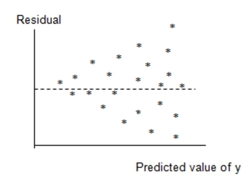
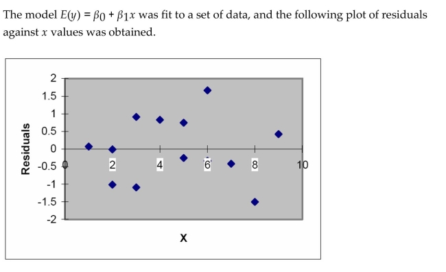
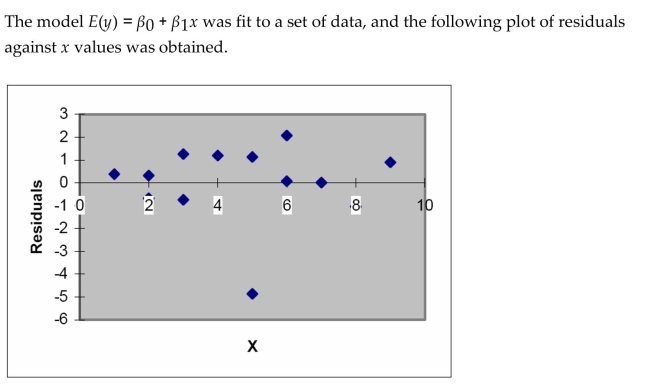
 Which of the following assumptions appears violated based on this plot?
A) The variance of the errors is constant
B) The errors are independent
C) The mean of the errors is zero
D) The errors are normally distributed
Question
Question
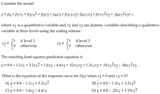
Consider the second-order model 
Question
What relationship between x and y is suggested by the scattergram? 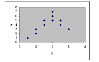
A) a quadratic relationship with downward concavity
B) a linear relationship with negative slope
C) a linear relationship with positive slope
D) a quadratic relationship with upward concavity
A) a quadratic relationship with downward concavity
B) a linear relationship with negative slope
C) a linear relationship with positive slope
D) a quadratic relationship with upward concavity
Question
Question
Question
Question
Question
Question
Question
Question
Question
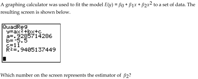
A) 11
B) .9286
C) 5.5
D) .9405
Question
Question
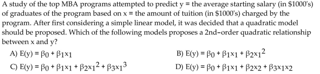
A study of the top MBA programs attempted to predict the average starting salary (in $1000's) of graduates of the program based on the amount of tuition (in $1000's) charged by the program and The average GMAT score of the program's students. The results of a regression analysis based on a Sample of 75 MBA programs is shown below: Least Squares Linear Regression of Salary
The model was then used to create 95% confidence and prediction intervals for y and for E(Y) when The tuition charged by the MBA program was $75,000 and the GMAT score was 675. The results are Shown here:
95% confidence interval for E(Y): ($126,610, $136,640)
95% prediction interval for Y: ($90,113, $173,160)
Which of the following interpretations is correct if you want to use the model to estimate E(Y) for All MBA programs?
A) We are 95% confident that the average starting salary for graduates of a single MBA program that charges $75,000 in tuition and has an average GMAT score of 675 will fall between
$90,113 and $173,16,30.
B) We are 95% confident that the average starting salary for graduates of a single MBA program that charges $75,000 in tuition and has an average GMAT score of 675 will fall between
$126,610 and $136,640.
C) We are 95% confident that the average of all starting salaries for graduates of all MBA programs that charge $75,000 in tuition and have an average GMAT score of 675 will fall
Between $126,610 and $136,640.
D) We are 95% confident that the average of all starting salaries for graduates of all MBA programs that charge $75,000 in tuition and have an average GMAT score of 675 will fall
Between $90,113 and $173,16,30.
Question
Question
Question
Question
Question
Question
Question

A) 4.2
B) 10.8
C) 11.4
D) 1.8
Question
Question
Question
Question
The first-order model below was fit to a set of data.  Explain how to determine if the constant variance assumption is satisfied.
Explain how to determine if the constant variance assumption is satisfied. Question
Question
Question
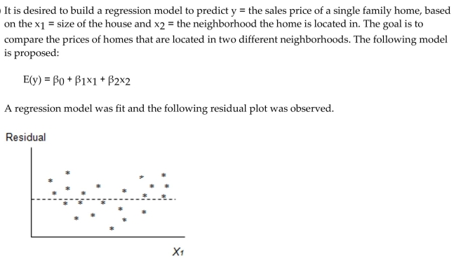
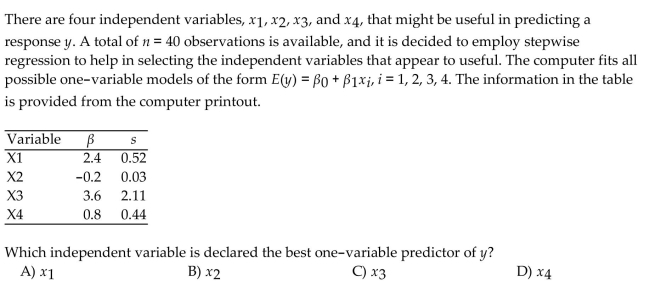
A public health researcher wants to use regression to predict the sun safety knowledge of pre-school children. The researcher randomly sampled 35 preschoolers, assigned them to one of two groups, and then measured the following three variables:
SUNSCORE: Score on sun-safety comprehension test
READING: Reading comprehension score
GROUP: if child received a Be Sun Safe demonstration, 0 if not
A regression model was fit and the following residual plot was observed.
Predicted value of
Which of the following assumptions appears violated based on this plot?
A) The errors are normally distributed
B) The errors are independent
C) The mean of the errors is zero
D) The variance of the errors is constant
Question
Question
Question
Question
Question
Question
Question
Question
Question

A) 1
B) 10
C) 16
D) 13
Question
Question
Question
A fast food chain test marketing a new sandwich chose 18 of its stores in one major
metropolitan area. Nine of the stores were in malls and nine were free standing. The sandwich was offered at three different introductory prices. The table shows the number of new sandwiches sold at each location for each location type and price combination.
Number of New Sandwiches Sold
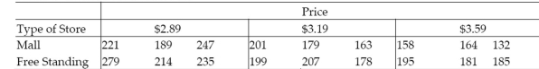
a. Write a model for the mean number of sandwiches sold, , assuming that the relationship between and price, , is first-order.
b. Fit the model to the data.
c. Write the prediction equations for mall and free-standing stores.
d. Do the data provide sufficient evidence that the change in number of sandwiches sold with respect to price is different for mall and free-standing stores? Use .
metropolitan area. Nine of the stores were in malls and nine were free standing. The sandwich was offered at three different introductory prices. The table shows the number of new sandwiches sold at each location for each location type and price combination.
Number of New Sandwiches Sold
a. Write a model for the mean number of sandwiches sold, , assuming that the relationship between and price, , is first-order.
b. Fit the model to the data.
c. Write the prediction equations for mall and free-standing stores.
d. Do the data provide sufficient evidence that the change in number of sandwiches sold with respect to price is different for mall and free-standing stores? Use .
Question
Question
Question
Question
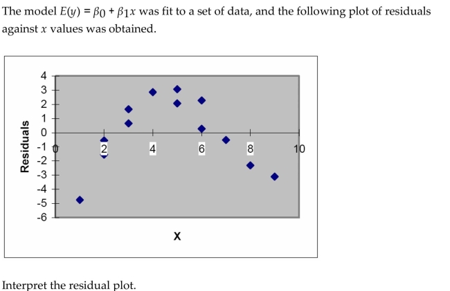
 Interpret the residual plot.
 Question
Question
Question
Question
 Interpret the residual plot.
 Question
Question
Question
Question
Question
Question
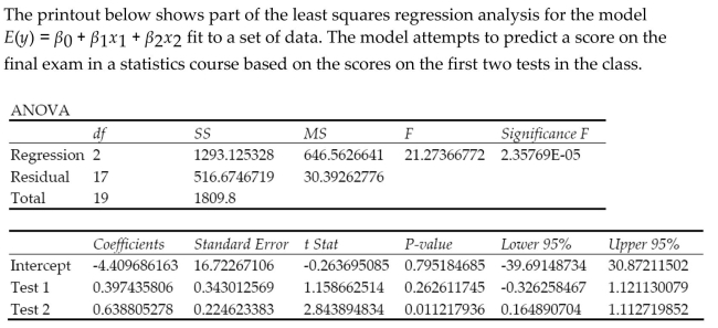 Is there evidence of multicollinearity in the printout? Explain.
 Question
Question
Question
Question
Question
Question
Question
Question
Question
Question
Question
Question
Question
Question
Question

Question
Question
A) The model is statistically useful for predicting Test4 score.
B) The model is not statistically useful for predicting Test4 score.
C) The first three test scores are reliable predictors of Test4 score.
D) The first three test scores are poor predictors of Test4 score.
Question
Question
Question
Question
Question
Question
Question
Question

Unlock Deck
Sign up to unlock the cards in this deck!
Unlock Deck
Unlock Deck
1/131
Play
Full screen (f)
Deck 12: Multiple Regression and Model Building
1
Which of the following assumptions appears violated based on this plot?A) The variance of the errors is constant
B) The errors are independent
C) The mean of the errors is zero
D) The errors are normally distributed
C
2
C
3
Consider the second-order model
B
4
What relationship between x and y is suggested by the scattergram?
A) a quadratic relationship with downward concavity
B) a linear relationship with negative slope
C) a linear relationship with positive slope
D) a quadratic relationship with upward concavity
A) a quadratic relationship with downward concavity
B) a linear relationship with negative slope
C) a linear relationship with positive slope
D) a quadratic relationship with upward concavity
Unlock Deck
Unlock for access to all 131 flashcards in this deck.
Unlock Deck
k this deck
5
A study of the top MBA programs attempted to predict the average starting salary (in $1000's) of graduates of the program based on the amount of tuition (in $1000's) charged by the program and The average GMAT score of the program's students. The results of a regression analysis based on a Sample of 75 MBA programs is shown below:
The global-f test statistic is shown on the printout to be the value . Interpret this value.
A) There is insufficient evidence, at , to indicate that at least one of the variables proposed in the interaction model is useful at predicting the average starting salary of graduates of MBA programs.
B) There is sufficient evidence, at , to indicate that at least one of the variables proposed in the interaction model is useful at predicting the average starting salary of graduates of MBA programs.
C) There is sufficient evidence, at , to indicate that there is a linear relationship between average starting salary of graduates of MBA programs and the tuition of the MBA program.
D) There is sufficient evidence, at , to indicate that there is a curvilinear relationship between average starting salary of graduates of MBA programs and the tuition of the MBA program.
Unlock Deck
Unlock for access to all 131 flashcards in this deck.
Unlock Deck
k this deck
6
A study of the top MBA programs attempted to predict the average starting salary (in $1000's) of graduates of the program based on the amount of tuition (in $1000's) charged by the program and the average GMAT score of the program's students. The results of a regression analysis based on a sample of 75 MBA programs is shown below: Least Squares Linear Regression of Salary
Interpret the p-value for the global f-test shown on the printout.
A) At ? = 0.05, there is sufficient evidence to indicate that something in the regression model is useful for predicting the average starting salary of the graduates of an MBA program.
B) At ? = 0.05, there is insufficient evidence to indicate that the average GMAT score of the MBA program's students is useful for predicting the average starting salary of the graduates of an
MBA program.
C) At ? = 0.05, there is sufficient evidence to indicate that the average GMAT score of the MBA program's students is useful for predicting the average starting salary of the graduates of an
MBA program.
D) At ? = 0.05, there is insufficient evidence to indicate that something in the regression model is useful for predicting the average starting salary of the graduates of an MBA program.
Unlock Deck
Unlock for access to all 131 flashcards in this deck.
Unlock Deck
k this deck
7
Unlock Deck
Unlock for access to all 131 flashcards in this deck.
Unlock Deck
k this deck
8
A study of the top MBA programs attempted to predict the average starting salary (in $1000's) of graduates of the program based on the amount of tuition (in $1000's) charged by the program and the average GMAT score of the program's students. The results of a regression analysis based on a sample of 75 MBA programs is shown below: Least Squares Linear Regression of Salary
Identify the test statistic that should be used to test to determine if the amount of tuition charged by a program is a useful predictor of the average starting salary of the graduates of the program.
A)
B)
C)
D)
Identify the test statistic that should be used to test to determine if the amount of tuition charged by a program is a useful predictor of the average starting salary of the graduates of the program.
A)
B)
C)
D)
Unlock Deck
Unlock for access to all 131 flashcards in this deck.
Unlock Deck
k this deck
9
A public health researcher wants to use regression to predict the sun safety knowledge of pre-school children. The researcher randomly sampled 35 preschoolers, assigned them to one of Two groups, and then measured the following three variables:
SUNSCORE: Score on sun-safety comprehension test
READING: Reading comprehension score
GROUP: if child received a Be Sun Safe demonstration, 0 if not
The following two models were hypothesized:
Model 1:
Model 2:
A partial f-test was conducted to compare the two models and the resulting p-value was found to be 0.0023. Fill in the blank. The results lead us to conclude that there is _____
A) insufficient evidence of quadratic relationship between sun-safety score to reading score.
B) sufficient evidence of a statistically useful model for sun-safety score.
C) sufficient evidence of interaction between sun-safety score and reading score.
D) sufficient evidence of a quadratic relationship between sun-safety score to reading score.
Unlock Deck
Unlock for access to all 131 flashcards in this deck.
Unlock Deck
k this deck
10
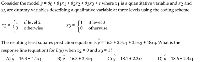
We decide to conduct a multiple regression analysis to predict the attendance at a major league baseball game. We use the size of the stadium as a quantitative independent variable and the type Of game as a qualitative variable (with two levels - day game or night game). We hypothesize the
Following model:
Where size of the stadium
if a day game, 0 if a night game
A plot of the relationship would show:
A) Two non-parallel curves
B) Two parallel lines
C) Two parallel curves
D) Two non-parallel lines
Following model:
Where size of the stadium
if a day game, 0 if a night game
A plot of the relationship would show:
A) Two non-parallel curves
B) Two parallel lines
C) Two parallel curves
D) Two non-parallel lines
Unlock Deck
Unlock for access to all 131 flashcards in this deck.
Unlock Deck
k this deck
11
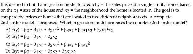
Which equation represents a complete second-order model for two quantitative independent variables?
A)
B)
C)
D)
A)
B)
C)
D)
Unlock Deck
Unlock for access to all 131 flashcards in this deck.
Unlock Deck
k this deck
12
Unlock Deck
Unlock for access to all 131 flashcards in this deck.
Unlock Deck
k this deck
13
A) 11
B) .9286
C) 5.5
D) .9405
Unlock Deck
Unlock for access to all 131 flashcards in this deck.
Unlock Deck
k this deck
14
Which of the following is not a possible indicator of multicollinearity?
A) significant correlations between pairs of independent variables
B) non-significant t-tests for individual β parameters when the F-test for overall model adequacy is significant
C) signs opposite from what is expected in the estimated β parameters
D) non-random patterns in the plot of the residuals versus the fitted values
Unlock Deck
Unlock for access to all 131 flashcards in this deck.
Unlock Deck
k this deck
15
A study of the top MBA programs attempted to predict the average starting salary (in $1000's) of graduates of the program based on the amount of tuition (in $1000's) charged by the program and The average GMAT score of the program's students. The results of a regression analysis based on a Sample of 75 MBA programs is shown below: Least Squares Linear Regression of Salary
The model was then used to create 95% confidence and prediction intervals for y and for E(Y) when The tuition charged by the MBA program was $75,000 and the GMAT score was 675. The results are Shown here:
95% confidence interval for E(Y): ($126,610, $136,640)
95% prediction interval for Y: ($90,113, $173,160)
Which of the following interpretations is correct if you want to use the model to estimate E(Y) for All MBA programs?
A) We are 95% confident that the average starting salary for graduates of a single MBA program that charges $75,000 in tuition and has an average GMAT score of 675 will fall between
$90,113 and $173,16,30.
B) We are 95% confident that the average starting salary for graduates of a single MBA program that charges $75,000 in tuition and has an average GMAT score of 675 will fall between
$126,610 and $136,640.
C) We are 95% confident that the average of all starting salaries for graduates of all MBA programs that charge $75,000 in tuition and have an average GMAT score of 675 will fall
Between $126,610 and $136,640.
D) We are 95% confident that the average of all starting salaries for graduates of all MBA programs that charge $75,000 in tuition and have an average GMAT score of 675 will fall
Between $90,113 and $173,16,30.
The model was then used to create 95% confidence and prediction intervals for y and for E(Y) when The tuition charged by the MBA program was $75,000 and the GMAT score was 675. The results are Shown here:
95% confidence interval for E(Y): ($126,610, $136,640)
95% prediction interval for Y: ($90,113, $173,160)
Which of the following interpretations is correct if you want to use the model to estimate E(Y) for All MBA programs?
A) We are 95% confident that the average starting salary for graduates of a single MBA program that charges $75,000 in tuition and has an average GMAT score of 675 will fall between
$90,113 and $173,16,30.
B) We are 95% confident that the average starting salary for graduates of a single MBA program that charges $75,000 in tuition and has an average GMAT score of 675 will fall between
$126,610 and $136,640.
C) We are 95% confident that the average of all starting salaries for graduates of all MBA programs that charge $75,000 in tuition and have an average GMAT score of 675 will fall
Between $126,610 and $136,640.
D) We are 95% confident that the average of all starting salaries for graduates of all MBA programs that charge $75,000 in tuition and have an average GMAT score of 675 will fall
Between $90,113 and $173,16,30.
Unlock Deck
Unlock for access to all 131 flashcards in this deck.
Unlock Deck
k this deck
16
Unlock Deck
Unlock for access to all 131 flashcards in this deck.
Unlock Deck
k this deck
17
Unlock Deck
Unlock for access to all 131 flashcards in this deck.
Unlock Deck
k this deck
18
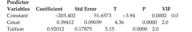
A study of the top MBA programs attempted to predict the average starting salary (in $1000's) of graduates of the program based on the amount of tuition (in $1000's) charged by the program and the average GMAT score of the program's students. The results of a regression analysis based on a sample of 75 MBA programs is shown below:
Interpret the coefficient for the tuition variable shown on the printout.
A) For every $1000 increase in the tuition charged by the MBA program, we estimate that the average starting salary will increase by $920.12, holding the GMAT score constant
B) For every $1000 increase in the tuition charged by the MBA program, we estimate that the average starting salary will increase by $394.12, holding the GMAT score constant
C) For every $1000 increase in the tuition charged by the MBA program, we estimate that the average starting salary will decrease by $203,402, holding the GMAT score constant.
D) For every $1000 increase in the average starting salary, we estimate that the tuition charged by the MBA program will increase by $920.12.
Unlock Deck
Unlock for access to all 131 flashcards in this deck.
Unlock Deck
k this deck
19
A study of the top MBA programs attempted to predict the average starting salary (in $1000's) of graduates of the program based on the amount of tuition (in $1000's) charged by the program and the average GMAT score of the program's students. The results of a regression analysis based on a sample of 75 MBA programs is shown below:
Least Squares Linear Regression of Salary
One of the t-test test statistics is shown on the printout to be the value . Interpret this value.
A) There is sufficient evidence, at , to indicate that at least one of the variables proposed in the interaction model is useful at predicting the average starting salary of graduates of MBA programs.
B) There is sufficient evidence, at , to indicate that there is a linear relationship between average starting salary of graduates of MBA programs and the tuition of the MBA program.
C) There is insufficient evidence, at , to indicate that at least one of the variables proposed in the interaction model is useful at predicting the average starting salary of graduates of MBA programs.
D) There is sufficient evidence, at , to indicate that there is a curvilinear relationship between average starting salary of graduates of MBA programs and the tuition of the MBA program.
Unlock Deck
Unlock for access to all 131 flashcards in this deck.
Unlock Deck
k this deck
20
Unlock Deck
Unlock for access to all 131 flashcards in this deck.
Unlock Deck
k this deck
21
Consider the partial printout below.
Unlock Deck
Unlock for access to all 131 flashcards in this deck.
Unlock Deck
k this deck
22
A) 4.2
B) 10.8
C) 11.4
D) 1.8
Unlock Deck
Unlock for access to all 131 flashcards in this deck.
Unlock Deck
k this deck
23
It is dangerous to predict outside the range of the data collected in a regression analysis. For instance, we shouldn't predict the price of a 5000 square foot home if all our sample homes were smaller than 4500 square feet. Which of the following multiple regression pitfalls does this example describe?
A) Estimability
B) Multicollinearity
C) Stepwise Regression
D) Extrapolation
A) Estimability
B) Multicollinearity
C) Stepwise Regression
D) Extrapolation
Unlock Deck
Unlock for access to all 131 flashcards in this deck.
Unlock Deck
k this deck
24
A study of the top MBA programs attempted to predict the average starting salary (in $1000's) of graduates of the program based on the amount of tuition (in $1000's) charged by the program and the average GMAT score of the program's students. The results of a regression analysis based on a sample of 75 MBA programs is shown below:
Least Squares Linear Regression of Salary
A) At , there is insufficient evidence to indicate that something in the regression model is useful for predicting the average starting salary of the graduates of an MBA program.
B) We expect most of the average starting salaries to fall within of their least squares predicted values.
C) We expect most of the average starting salaries to fall within of their least squares predicted values.
D) We can explain of the variation in the average starting salaries around their mean using the model that includes the average GMAT score and the tuition for the MBA program.
Unlock Deck
Unlock for access to all 131 flashcards in this deck.
Unlock Deck
k this deck
25
Retail price data for hard disk drives were recently reported in a computer magazine. Three variables were recorded for each hard disk drive:
Retail PRICE (measured in dollars)
Microprocessor SPEED (measured in megahertz)
(Values in sample range from 10 to 40 )
size (measured in computer processing units)
(Values in sample range from 286 to 486 )
A first-order regression model was fit to the data. Part of the printout follows:
Parameter Estimates
PARAMETER STANDARD T FOR 0:
VARIABLE DF ESTIMATE ERROR PARAMETER PROB
Identify and interpret the estimate for the SPEED -coefficient, .
A) ; For every 1-megahertz increase in SPEED, we estimate PRICE to increase , holding CHIP fixed.
B) ; For every 1-megahertz increase in SPEED, we estimate PRICE (y) to increase , holding CHIP fixed.
C) ; For every increase in PRICE, we estimate SPEED to increase 105 megahertz, holding CHIP fixed.
D) ; For every increase in PRICE, we estimate SPPED to increase by about 4 megahertz, holding CHIP fixed.
Unlock Deck
Unlock for access to all 131 flashcards in this deck.
Unlock Deck
k this deck
26
The first-order model below was fit to a set of data. Explain how to determine if the constant variance assumption is satisfied.
Explain how to determine if the constant variance assumption is satisfied. Unlock Deck
Unlock for access to all 131 flashcards in this deck.
Unlock Deck
k this deck
27
Twenty colleges each recommended one of its graduating seniors for a prestigious graduate fellowship. The process to determine which student will receive the fellowship includes several interviews. The gender of each student and his or her score on the first interview are shown below.
a. Suppose you want to use gender to model the score on the interview y. Create the
appropriate number of dummy variables for gender and write the model.
b. Fit the model to the data.
c. Give the null hypothesis for testing whether gender is a useful predictor of the score y.
d. Conduct the test and give the appropriate conclusion
Unlock Deck
Unlock for access to all 131 flashcards in this deck.
Unlock Deck
k this deck
28
Retail price data for n = 60 hard disk drives were recently reported in a computer magazine. Three variables were recorded for each hard disk drive:
A first-order regression model. was fit to the data. Part of the printout follows:
Parameter Estimates
PARAMETER STANDARD T FOR 0 :
VARIABLE DF ESTIMATE ERROR PARAMETER PROB
A first-order regression model. was fit to the data. Part of the printout follows:
Parameter Estimates
PARAMETER STANDARD T FOR 0 :
VARIABLE DF ESTIMATE ERROR PARAMETER PROB
Unlock Deck
Unlock for access to all 131 flashcards in this deck.
Unlock Deck
k this deck
29
A public health researcher wants to use regression to predict the sun safety knowledge of pre-school children. The researcher randomly sampled 35 preschoolers, assigned them to one of two groups, and then measured the following three variables:
SUNSCORE: Score on sun-safety comprehension test
READING: Reading comprehension score
GROUP: if child received a Be Sun Safe demonstration, 0 if not
A regression model was fit and the following residual plot was observed.
Predicted value of
Which of the following assumptions appears violated based on this plot?
A) The errors are normally distributed
B) The errors are independent
C) The mean of the errors is zero
D) The variance of the errors is constant
SUNSCORE: Score on sun-safety comprehension test
READING: Reading comprehension score
GROUP: if child received a Be Sun Safe demonstration, 0 if not
A regression model was fit and the following residual plot was observed.
Predicted value of
Which of the following assumptions appears violated based on this plot?
A) The errors are normally distributed
B) The errors are independent
C) The mean of the errors is zero
D) The variance of the errors is constant
Unlock Deck
Unlock for access to all 131 flashcards in this deck.
Unlock Deck
k this deck
30
Consider the partial printout for an interaction regression analysis of the relationship between a dependent variable and two independent variables and .
ANOVA
a. Write the prediction equation for the interaction model.
b. Test the overall utility of the interaction model using the global -test at .
c. Test the hypothesis (at ) that and interact positively.
d. Estimate the change in for each additional 1-unit increase in when .
ANOVA
a. Write the prediction equation for the interaction model.
b. Test the overall utility of the interaction model using the global -test at .
c. Test the hypothesis (at ) that and interact positively.
d. Estimate the change in for each additional 1-unit increase in when .
Unlock Deck
Unlock for access to all 131 flashcards in this deck.
Unlock Deck
k this deck
31
A study of the top MBA programs attempted to predict the average starting salary (in $1000's) of graduates of the program based on the amount of tuition (in $1000's) charged by the program and the average GMAT score of the program's students. The results of a regression analysis based on a sample of 75 MBA programs is shown below:
The model was then used to create 95% confidence and prediction intervals for y and for E(Y) when the tuition charged by the MBA program was $75,000 and the GMAT score was 675. The results are shown here:
95% confidence interval for E(Y): ($126,610, $136,640)
95% prediction interval for Y: ($90,113, $173,160)
Which of the following interpretations is correct if you want to use the model to estimate Y for a single MBA program?
A) We are 95% confident that the average of all starting salaries for graduates of all MBA programs that charge $75,000 in tuition and have an average GMAT score of 675 will fall
Between $126,610 and $136,640.
B) We are 95% confident that the average starting salary for graduates of a single MBA program that charges $75,000 in tuition and has an average GMAT score of 675 will fall between
$126,610 and $136,640.
C) We are 95% confident that the average starting salary for graduates of a single MBA program that charges $75,000 in tuition and has an average GMAT score of 675 will fall between
$90,113 and $173,16,30.
D) We are 95% confident that the average of all starting salaries for graduates of all MBA programs that charge $75,000 in tuition and have an average GMAT score of 675 will fall
Between $90,113 and $173,16,30.
Unlock Deck
Unlock for access to all 131 flashcards in this deck.
Unlock Deck
k this deck
32
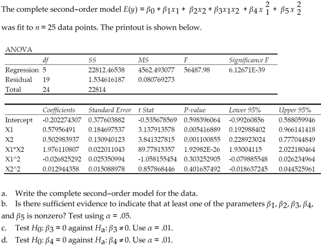
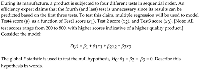
During its manufacture, a product is subjected to four different tests in sequential order. An efficiency expert claims that the fourth (and last) test is unnecessary since its results can be predicted based on the first three tests. To test this claim, multiple regression will be used to model Test4 score , as a function of Test1 score , Test 2 score , and Test3 score . [Note: All test scores range from 200 to 800 , with higher scores indicative of a higher quality product.] Consider the model:
The first-order model was fit to the data for each of 12 units sampled from the production line. The results are summarized in the printout.
Suppose the confidence interval for is . Which of the following statements is incorrect?
A) We are confident that the Test 3 is a useful linear predictor of Test 4 score, holding Test1 and Test2 fixed.
B) At , there is insufficient evidence to reject in favor of .
C) We are confident that the increase in Test4 score for every 1-point increase in Test3 score falls between and , holding Test1 and Test 2 fixed.
D) We are confident that the estimated slope for the Test4-Test3 line falls between and holding Test1 and Test2 fixed.
Unlock Deck
Unlock for access to all 131 flashcards in this deck.
Unlock Deck
k this deck
33
The confidence interval for the mean E(y) is narrower that the prediction interval for y.
Unlock Deck
Unlock for access to all 131 flashcards in this deck.
Unlock Deck
k this deck
34
Unlock Deck
Unlock for access to all 131 flashcards in this deck.
Unlock Deck
k this deck
35
Unlock Deck
Unlock for access to all 131 flashcards in this deck.
Unlock Deck
k this deck
36
Unlock Deck
Unlock for access to all 131 flashcards in this deck.
Unlock Deck
k this deck
37
In regression, it is desired to predict the dependent variable based on values of other related independent variables. Occasionally, there are relationships that exist between the independent variables. Which of the following multiple regression pitfalls does this example describe?
A) Multicollinearity
B) Extrapolation
C) Stepwise Regression
D) Estimability
A) Multicollinearity
B) Extrapolation
C) Stepwise Regression
D) Estimability
Unlock Deck
Unlock for access to all 131 flashcards in this deck.
Unlock Deck
k this deck
38
A) 1
B) 10
C) 16
D) 13
Unlock Deck
Unlock for access to all 131 flashcards in this deck.
Unlock Deck
k this deck
39
A study of the top MBA programs attempted to predict the average starting salary (in $1000's) of graduates of the program based on the amount of tuition (in $1000's) charged by the program and the average GMAT score of the program's students. The results of a regression analysis based on a sample of 75 MBA programs is shown below:
Cases Included 75 Missing Cases 0 One of the t-test test statistics is shown on the printout to be value . Interpret this value.
A) There is sufficient evidence, at , to indicate that the interaction between average tuition and average GMAT score is a useful predictor of the average starting salary of graduates of MBA programs.
B) There is insufficient evidence, at , to indicate that at least one of the variables proposed in the interaction model is useful at predicting the average starting salary of graduates of MBA programs.
C) There is sufficient evidence, at , to indicate that at least one of the variables proposed in the interaction model is useful at predicting the average starting salary of graduates of MBA programs.
D) There is insufficient evidence, at , to indicate that the interaction between average tuition and average GMAT score is a useful predictor of the average starting salary of graduates of MBA programs.
Unlock Deck
Unlock for access to all 131 flashcards in this deck.
Unlock Deck
k this deck
40
A study of the top MBA programs attempted to predict the average starting salary (in $1000's) of graduates of the program based on the amount of tuition (in $1000's) charged by the program and the average GMAT score of the program's students. The results of a regression analysis based on a sample of 75 MBA programs is shown below:
Cases Included 75 Missing Cases 0
The global-f test statistic is shown on the printout to be the value . Interpret this value.
A) There is sufficient evidence, at , to indicate that at least one of the variables proposed in the interaction model is useful at predicting the average starting salary of graduates of MBA programs.
B) There is insufficient evidence, at , to indicate that at least one of the variables proposed in the interaction model is useful at predicting the average starting salary of graduates of MBA programs.
C) There is insufficient evidence, at , to indicate that the interaction between average tuition and average GMAT score is a useful predictor of the average starting salary of graduates of MBA programs.
D) There is sufficient evidence, at , to indicate that the interaction between average tuition and average GMAT score is a useful predictor of the average starting salary of graduates of MBA programs.
Unlock Deck
Unlock for access to all 131 flashcards in this deck.
Unlock Deck
k this deck
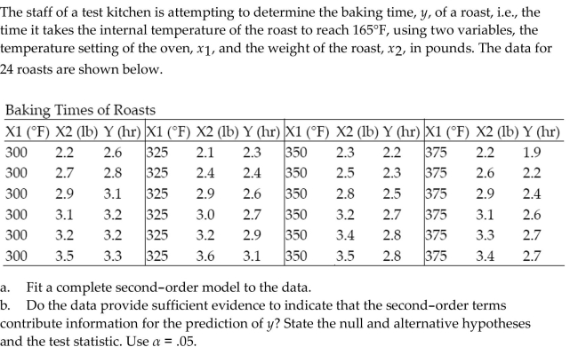
41
A fast food chain test marketing a new sandwich chose 18 of its stores in one major
metropolitan area. Nine of the stores were in malls and nine were free standing. The sandwich was offered at three different introductory prices. The table shows the number of new sandwiches sold at each location for each location type and price combination.
Number of New Sandwiches Sold
a. Write a model for the mean number of sandwiches sold, , assuming that the relationship between and price, , is first-order.
b. Fit the model to the data.
c. Write the prediction equations for mall and free-standing stores.
d. Do the data provide sufficient evidence that the change in number of sandwiches sold with respect to price is different for mall and free-standing stores? Use .
Unlock Deck
Unlock for access to all 131 flashcards in this deck.
Unlock Deck
k this deck
42
The concessions manager at a beachside park recorded the high temperature, the number of people at the park, and the number of bottles of water sold for each of 12 consecutive saturdays. The data are shown below. a. Fit the model to the data, letting represent the number of bottles of water sold, the temperature, and the number of people at the park.
b. Find the confidence interval for the mean number of bottles of water sold when the temperature is and there are 2700 people at the park.
c. Find the prediction interval for the number of bottles of water sold when the temperature is and there are 2700 people at the park.
b. Find the confidence interval for the mean number of bottles of water sold when the temperature is and there are 2700 people at the park.
c. Find the prediction interval for the number of bottles of water sold when the temperature is and there are 2700 people at the park.
Unlock Deck
Unlock for access to all 131 flashcards in this deck.
Unlock Deck
k this deck
43
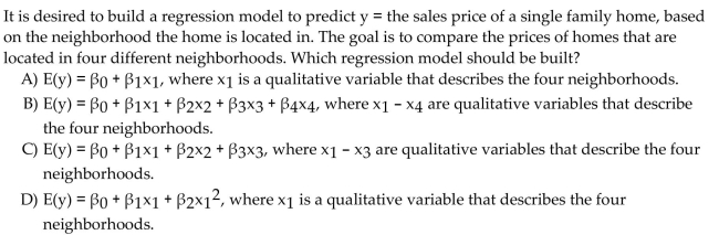
In Hawaii, proceedings are under way to enable private citizens to own the property that their homes are built on. In prior years, only estates were permitted to own land, and homeowners leased the land from the estate. In order to comply with the new law, a large Hawaiian estate wants to use regression analysis to estimate the fair market value of the land. The following variables are proposed:
if property near Cove, 0 if not Write a regression model relating the sale price of a property to the qualitative variable x. Interpret all the ?s in the model.
if property near Cove, 0 if not Write a regression model relating the sale price of a property to the qualitative variable x. Interpret all the ?s in the model.
Unlock Deck
Unlock for access to all 131 flashcards in this deck.
Unlock Deck
k this deck
44
Unlock Deck
Unlock for access to all 131 flashcards in this deck.
Unlock Deck
k this deck
45
Interpret the residual plot. Unlock Deck
Unlock for access to all 131 flashcards in this deck.
Unlock Deck
k this deck
46
A college admissions officer proposes to use regression to model a student's college GPA at graduation in terms of the following two variables: The admissions officer believes the relationship between college GPA and high school GPA is linear and the relationship between SAT score and college GPA is linear. She also believes that the relationship between college GPA and high school GPA depends on the student's SAT score. Write the regression model she should fit.
Unlock Deck
Unlock for access to all 131 flashcards in this deck.
Unlock Deck
k this deck
47
A certain type of rare gem serves as a status symbol for many of its owners. In theory, for low prices, the demand decreases as the price of the gem increases. However, experts hypothesize that when the gem is valued at very high prices, the demand increases with price due to the status the owners believe they gain by obtaining the gem. Thus, the model proposed to best explain the demand for the gem by its price is the quadratic model
where Demand (in thousands) and Retail price per carat (dollars).
This model was fit to data collected for a sample of 12 rare gems. A portion of the printout is given below:
Is there sufficient evidence to indicate the model is useful for predicting the demand for the gem? Use .
where Demand (in thousands) and Retail price per carat (dollars).
This model was fit to data collected for a sample of 12 rare gems. A portion of the printout is given below:
Is there sufficient evidence to indicate the model is useful for predicting the demand for the gem? Use .
Unlock Deck
Unlock for access to all 131 flashcards in this deck.
Unlock Deck
k this deck
48
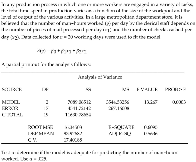
In any production process in which one or more workers are engaged in a variety of tasks, the total time spent in production varies as a function of the size of the workpool and the level of output of the various activities. In a large metropolitan department store, it is believed that the number of man-hours worked per day by the clerical staff depends on the number of pieces of mail processed per day and the number of checks cashed per day . Data collected for working days were used to fit the model:
A printout for the analysis follows:
Parameter Estimates
PARAMETER STANDARD T FOR 0:
VARIABLE DF ESTIMATE ERROR PARAMETER PROB
Test to determine if there is a positive linear relationship between the number of man-hours worked, , and the number of checks cashed per day, . Use .
A printout for the analysis follows:
Parameter Estimates
PARAMETER STANDARD T FOR 0:
VARIABLE DF ESTIMATE ERROR PARAMETER PROB
Test to determine if there is a positive linear relationship between the number of man-hours worked, , and the number of checks cashed per day, . Use .
Unlock Deck
Unlock for access to all 131 flashcards in this deck.
Unlock Deck
k this deck
49
Interpret the residual plot. Unlock Deck
Unlock for access to all 131 flashcards in this deck.
Unlock Deck
k this deck
50
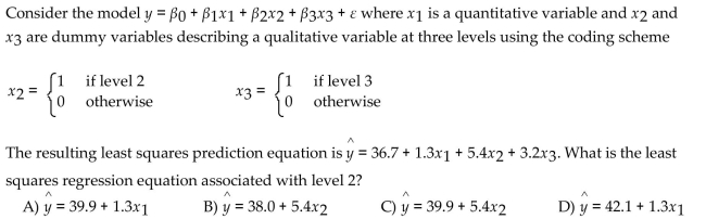
The model was used to relate to a single qualitative variable, where
This model was fit to data points and the following result was obtained:
a. Use the least squares prediction equation to find the estimate of for each level of the qualitative variable.
b. Specify the null and alternative hypothesis you would use to test whether is the same for all levels of the independent variable.
Unlock Deck
Unlock for access to all 131 flashcards in this deck.
Unlock Deck
k this deck
51
Retail price data for hard disk drives were recently reported in a computer magazine. Three variables were recorded for each hard disk drive:
Retail PRICE (measured in dollars)
Microprocessor SPEED (measured in megahertz)
(Values in sample range from 10 to 40 )
size (measured in computer processing units)
(Values in sample range from 286 to 486 )
A first-order regression model was fit to the data. Part of the printout follows:
Interpret the prediction interval for when and .
Unlock Deck
Unlock for access to all 131 flashcards in this deck.
Unlock Deck
k this deck
52
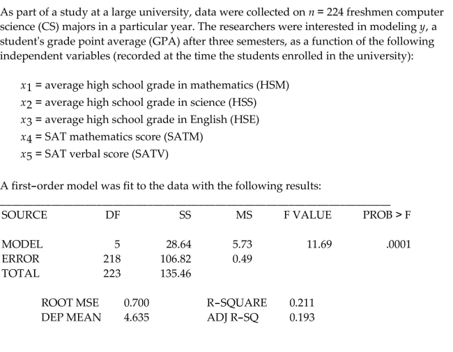
As part of a study at a large university, data were collected on freshmen computer science (CS) majors in a particular year. The researchers were interested in modeling , a student's grade point average (GPA) after three semesters, as a function of the following independent variables (recorded at the time the students enrolled in the university):
average high school grade in mathematics (HSM)
average high school grade in science (HSS)
average high school grade in English (HSE)
SAT mathematics score (SATM)
SAT verbal score (SATV)
A first-order model was fit to data with .
Interpret the value of the adjusted coefficient of determination .
average high school grade in mathematics (HSM)
average high school grade in science (HSS)
average high school grade in English (HSE)
SAT mathematics score (SATM)
SAT verbal score (SATV)
A first-order model was fit to data with .
Interpret the value of the adjusted coefficient of determination .
Unlock Deck
Unlock for access to all 131 flashcards in this deck.
Unlock Deck
k this deck
53
Consider the data given in the table below. a. Plot the data on a scattergram. Does a quadratic model seem to be a good fit for the
data? Explain.
b. Use the method of least squares to find a quadratic prediction equation.
c. Graph the prediction equation on your scattergram.
data? Explain.
b. Use the method of least squares to find a quadratic prediction equation.
c. Graph the prediction equation on your scattergram.
Unlock Deck
Unlock for access to all 131 flashcards in this deck.
Unlock Deck
k this deck
54
A certain type of rare gem serves as a status symbol for many of its owners. In theory, for low prices, the demand decreases as the price of the gem increases. However, experts hypothesize that when the gem is valued at very high prices, the demand increases with price due to the status the owners believe they gain by obtaining the gem. Thus, the model proposed to best explain the demand for the gem by its price is the quadratic model
where Demand (in thousands) and Retail price per carat (dollars). This model was fit to data collected for a sample of 12 rare gems. A portion of the printout is given below: Does the quadratic term contribute useful information for predicting the demand for the gem? Use .
Does the quadratic term contribute useful information for predicting the demand for the gem? Use .
Unlock Deck
Unlock for access to all 131 flashcards in this deck.
Unlock Deck
k this deck
55
Is there evidence of multicollinearity in the printout? Explain. Unlock Deck
Unlock for access to all 131 flashcards in this deck.
Unlock Deck
k this deck
56
Unlock Deck
Unlock for access to all 131 flashcards in this deck.
Unlock Deck
k this deck
57
Unlock Deck
Unlock for access to all 131 flashcards in this deck.
Unlock Deck
k this deck
58
Why is the random error term ? added to a multiple regression model?
Unlock Deck
Unlock for access to all 131 flashcards in this deck.
Unlock Deck
k this deck
59
A college admissions officer proposes to use regression to model a student's college GPA at graduation in terms of the following two variables: The admissions officer believes the relationship between college GPA and high school GPA is linear and the relationship between SAT score and college GPA is linear. She also believes that the relationship between college GPA and high school GPA depends on the student's SAT score. She proposes the regression model: Explain how to determine if the relationship between college GPA and SAT score depends on the high school GPA.
Unlock Deck
Unlock for access to all 131 flashcards in this deck.
Unlock Deck
k this deck
60
Unlock Deck
Unlock for access to all 131 flashcards in this deck.
Unlock Deck
k this deck
61
Consider the data given in the table below. Plot the data on a scattergram. Does a second-order model seem to be a good fit for the data? Explain.
Unlock Deck
Unlock for access to all 131 flashcards in this deck.
Unlock Deck
k this deck
62
The table shows the profit y (in thousands of dollars) that a company made during a month when the price of its product was x dollars per unit.
a. Fit the model to the data and give the least squares prediction equation.
b. Plot the fitted equation on a scattergram of the data.
c. Is there sufficient evidence of downward curvature in the relationship between profit and price? Use .
a. Fit the model to the data and give the least squares prediction equation.
b. Plot the fitted equation on a scattergram of the data.
c. Is there sufficient evidence of downward curvature in the relationship between profit and price? Use .
Unlock Deck
Unlock for access to all 131 flashcards in this deck.
Unlock Deck
k this deck
63
The model was used to relate to a single qualitative variable. How many levels does the qualitative variable have?
Unlock Deck
Unlock for access to all 131 flashcards in this deck.
Unlock Deck
k this deck
64
The table below shows data for observations.
a. Use a first-order regression model to find a least squares prediction equation for the model.
b. Find a confidence interval for the coefficient of in your model. Interpret the result.
c. Find a confidence interval for the coefficient of in your model. Interpret the result.
d. Find and and interpret these values.
e. Test the null hypothesis against the alternative hypothesis at least one . Use . Interpret the result.
Unlock Deck
Unlock for access to all 131 flashcards in this deck.
Unlock Deck
k this deck
65
A statistics professor gave three quizzes leading up to the first test in his class. The quiz grades and test grade for each of eight students are given in the table.
The professor would like to use the data to find a first-order model that he might use to predict a student's grade on the first test using that student's grades on the first threequizzes.
a. Identify the dependent and independent variables for the model.
b. What is the least squares prediction equation?
c. Find the SSE and the estimator of for the model.
Unlock Deck
Unlock for access to all 131 flashcards in this deck.
Unlock Deck
k this deck
66
Retail price data for hard disk drives were recently reported in a computer magazine. Three variables were recorded for each hard disk drive:
Retail PRICE (measured in dollars)
Microprocessor SPEED (measured in megahertz)
(Values in sample range from 10 to 40 )
CHIP size (measured in computer processing units)
(Values in sample range from 286 to 486 )
A first-order regression model was fit to the data. Part of the printout follows:
Test to determine if the model is adequate for predicting the price of a computer. Use .
Unlock Deck
Unlock for access to all 131 flashcards in this deck.
Unlock Deck
k this deck
67
The sum of squared errors (SSE) of a least squares regression model decreases when new terms are added to the model.
Unlock Deck
Unlock for access to all 131 flashcards in this deck.
Unlock Deck
k this deck
68
Unlock Deck
Unlock for access to all 131 flashcards in this deck.
Unlock Deck
k this deck
69
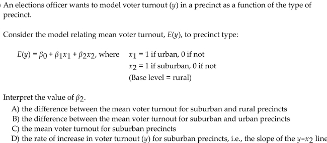
An elections officer wants to model voter turnout (y) in a precinct as a function of type of election, national or state.
Write a model for mean voter turnout, E(y), as a function of type of election.
A) , where if national, 0 if state
B) , where voter turnout
C) , where if national, 0 if not and if state, 0 if not
D) , where voter turnout
Write a model for mean voter turnout, E(y), as a function of type of election.
A) , where if national, 0 if state
B) , where voter turnout
C) , where if national, 0 if not and if state, 0 if not
D) , where voter turnout
Unlock Deck
Unlock for access to all 131 flashcards in this deck.
Unlock Deck
k this deck
70
Unlock Deck
Unlock for access to all 131 flashcards in this deck.
Unlock Deck
k this deck
71
Unlock Deck
Unlock for access to all 131 flashcards in this deck.
Unlock Deck
k this deck
72
A) The model is statistically useful for predicting Test4 score.
B) The model is not statistically useful for predicting Test4 score.
C) The first three test scores are reliable predictors of Test4 score.
D) The first three test scores are poor predictors of Test4 score.
Unlock Deck
Unlock for access to all 131 flashcards in this deck.
Unlock Deck
k this deck
73
In any production process in which one or more workers are engaged in a variety of tasks, the total time spent in production varies as a function of the size of the workpool and the level of output of the various activities. In a large metropolitan department store, it is believed that the number of man-hours worked per day by the clerical staff depends on the number of pieces of mail processed per day and the number of checks cashed per day . Data collected for working days were used to fit the model:
A partial printout for the analysis follows:
Interpret the 95% prediction interval for y shown on the printout.
A) We are 95% confident that the mean number of man-hours worked per day falls between 47.224 and 119.126 for all days in which 7,781 pieces of mail are processed and 644 checks are
Cashed.
B) We are 95% confident that the number of man-hours worked per day falls between 47.224 and 119.126.
C) We are 95% confident that between 47.224 and 119.126 man-hours will be worked during a single day in which 7,781 pieces of mail are processed and 644 checks are cashed.
D) We expect to predict number of man-hours worked per day to within an amount between 47.224 and 119.126 of the true value.
Unlock Deck
Unlock for access to all 131 flashcards in this deck.
Unlock Deck
k this deck
74
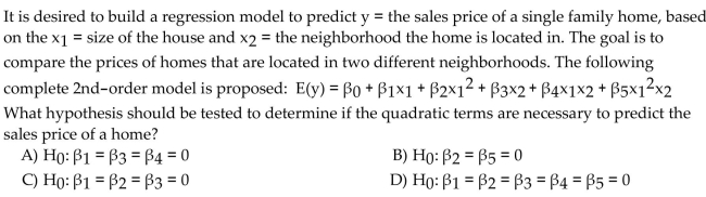
Operations managers often use work sampling to estimate how much time workers spend on each operation. Work sampling-which involves observing workers at random points in time-was applied to the staff of the catalog sales department of a clothing manufacturer.
The department applied regression to the following data collected for 40 consecutive working days:
TIME: Time spent (in hours) taking telephone orders during the day
ORDERS: Number of telephone orders received during the day
WEEK: weekday, 0 if Saturday or Sunday
Consider the complete 2nd-order model:
Explain how to conduct a test to determine if a quadratic relationship between total order time and the number of orders taken is necessary in the regression model above. Specify the null and alternative hypotheses that are to be tested.
Unlock Deck
Unlock for access to all 131 flashcards in this deck.
Unlock Deck
k this deck
75
A statistics professor gave three quizzes leading up to the first test in his class. The quiz grades and test grade for each of eight students are given in the table.
The professor fit a first-order model to the data that he intends to use to predict a student's grade on the first test using that student's grades on the first three quizzes.
Test the null hypothesis against the alternative hypothesis : at least one . Use . Interpret the result.
The professor fit a first-order model to the data that he intends to use to predict a student's grade on the first test using that student's grades on the first three quizzes.
Test the null hypothesis against the alternative hypothesis : at least one . Use . Interpret the result.
Unlock Deck
Unlock for access to all 131 flashcards in this deck.
Unlock Deck
k this deck
76
In stepwise regression, the probability of making one or more Type I or Type II errors is quite small.
Unlock Deck
Unlock for access to all 131 flashcards in this deck.
Unlock Deck
k this deck
77
The printout shows the results of a first-order regression analysis relating the sales price of a product to the time in hours and the cost of raw materials needed to make the product.
SUMMARY OUTPUT
ANOVA
a. What is the least squares prediction equation?
b. Identify the SSE from the printout.
c. Find the estimator of for the model.
SUMMARY OUTPUT
ANOVA
a. What is the least squares prediction equation?
b. Identify the SSE from the printout.
c. Find the estimator of for the model.
Unlock Deck
Unlock for access to all 131 flashcards in this deck.
Unlock Deck
k this deck
78
A collector of grandfather clocks believes that the price received for the clocks at an auction increases with the number of bidders, but at an increasing (rather than a constant) rate. Thus, the model proposed to best explain auction price (y, in dollars) by number of bidders (x) is the quadratic model
This model was fit to data collected for a sample of 32 clocks sold at auction; the resulting estimate of was .
Interpret this estimate of .
A) We estimate the auction price will increase for each additional bidder at the auction.
B) is a shift parameter that has no practical interpretation.
C) We estimate the auction price will be when there are no bidders at the auction.
D) We estimate the auction price will decrease for each additional bidder at the auction.
Unlock Deck
Unlock for access to all 131 flashcards in this deck.
Unlock Deck
k this deck
79
The method of fitting first-order models is the same as that of fitting the simple straight-line model, i.e. the method of least squares.
Unlock Deck
Unlock for access to all 131 flashcards in this deck.
Unlock Deck
k this deck
80
The concessions manager at a beachside park recorded the high temperature, the number of people at the park, and the number of bottles of water sold for each of 12 consecutiveSaturdays. The data are shown below.
a. Fit the model to the data, letting represent the number of bottles of water sold, the temperature, and the number of people at the park.
b. Identify at least two indicators of multicollinearity in the model.
c. Comment on the usefulness of the model to predict the number of bottles of water sold on a Saturday when the high temperature is and there are 3500 people at the park.
Unlock Deck
Unlock for access to all 131 flashcards in this deck.
Unlock Deck
k this deck
Unlock Deck
Unlock for access to all 131 flashcards in this deck.


