Deck 3: Statistics for Describing, Exploring, and Comparing Data
Full screen (f)
Question
Question
Question
Question
Question
Question
Question
Question
Question
Question
Question
Question
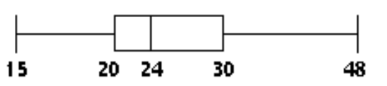
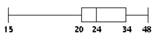
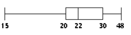
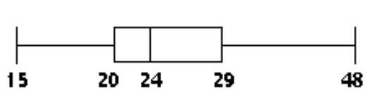
Describe any similarities or differences in the two distributions represented by the following boxplots. Assume the two boxplots have the same scale. 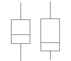
Question
Question
Question
Question
Question
Question
Question
Question
Question
Question
Describe any similarities or differences in the two distributions represented by the following boxplots. Assume the two boxplots have the same scale.

Question
Question
Question
Question
Question
Question
Question
Question
Question
Question
Question
Question
Question
Question
Question
Question
Question
Question
Question
Question
Question
Question
Question
Question
Question
Question
Question
Question
Question
Question
Question
Question
Question
Question
Question
Question
Question
Question
Question
Question
Question
Question
Question
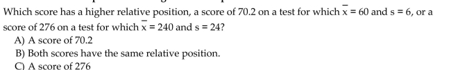
Determine which score corresponds to the higher relative position.
Question
Question
Question
Question
Question
Question
Question
Question
Question
Construct a boxplot for the given data. Include values of the 5-number summary in all boxplots.
-The ages of the 35 members of a track and field team are listed below. Construct a boxplot for the data set.
A)
B)
C)
D)
-The ages of the 35 members of a track and field team are listed below. Construct a boxplot for the data set.
A)
B)
C)
D)
Question
Question
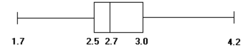
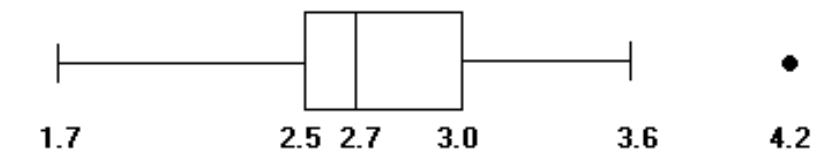
Construct a modified boxplot for the data. Identify any outliers.
-The weights (in ounces) of 27 tomatoes are listed below.
A) Outliers: 1.7 oz, 4.2 oz

B) No outliers
C) Outlier: 4.2 oz
D) Outliers: 1.7 oz, 3.6 oz, 4.2 oz
-The weights (in ounces) of 27 tomatoes are listed below.
A) Outliers: 1.7 oz, 4.2 oz
B) No outliers
C) Outlier: 4.2 oz
D) Outliers: 1.7 oz, 3.6 oz, 4.2 oz
Question
Question
Question
Question

Unlock Deck
Sign up to unlock the cards in this deck!
Unlock Deck
Unlock Deck
1/187
Play
Full screen (f)
Deck 3: Statistics for Describing, Exploring, and Comparing Data
1
The table below provides a frequency distribution for the winner of the Davis Cup during the period 1977-1994.
Which measure of center, the mean, the median, or the mode is most appropriate here? Why?
Which measure of center, the mean, the median, or the mode is most appropriate here? Why?
The mode. Since the data are not numerical, it is not possible to find the median or mean. The mode is the only measure of center that can be used with data at the nominal level of measurement.
2
Does the mode of a numerical data set always lie close to the median? Explain your answer and give an example of a data set to illustrate your answer.
No, the mode is the value that occurs most frequently and this value is not
necessarily close to the median. Examples will vary.
necessarily close to the median. Examples will vary.
3
Construct a data set for which the range is misleading as a measure of variation. Explain why the range is misleading and suggest an alternative measure of variation.
Answers will vary. The data set should contain an outlier, which will tend to make the range quite large even though the remaining data may be bunched fairly close together. In general, the standard deviation or variance are more reliable measures of variation.
4
Suppose that a state introduces a state income tax which will be at a flat rate of 3%. The state legislature wishes to estimate how much money they will receive in taxes, and to do this they need to know the average income of residents of the state. Which information would be most useful, the mean income, the median income, or the mode of the incomes? Why?
Unlock Deck
Unlock for access to all 187 flashcards in this deck.
Unlock Deck
k this deck
5
Skewness can be measured by Pearson's index of skewness:
If or , the data can be considered significantly skewed. Would you expect that incomes of all adults in the US would be skewed? In which direction? Why? Would you expect that for these incomes, Pearson's index of skewness would be greater than 1, smaller than , or between and 1 ?
If or , the data can be considered significantly skewed. Would you expect that incomes of all adults in the US would be skewed? In which direction? Why? Would you expect that for these incomes, Pearson's index of skewness would be greater than 1, smaller than , or between and 1 ?
Unlock Deck
Unlock for access to all 187 flashcards in this deck.
Unlock Deck
k this deck
6
The textbook defines unusual values as those data points with scores less than or scores greater than . Comment on this definition with respect to Chebyshev's theorem; refer specifically to the percent of scores which would be defined as unusual according to Chebyshev's theorem.
Unlock Deck
Unlock for access to all 187 flashcards in this deck.
Unlock Deck
k this deck
7
Describe how to find the percentile for a given score in a set of data. How does this process relate to the definition of a percentile score?
Unlock Deck
Unlock for access to all 187 flashcards in this deck.
Unlock Deck
k this deck
8
Heights of adult women are known to have a bell-shaped distribution. Draw a boxplot to illustrate the results.
Unlock Deck
Unlock for access to all 187 flashcards in this deck.
Unlock Deck
k this deck
9
Responses to a survey question about eye color are coded as 1 (for brown), 2 (for blue), 3 (for green), 4 (for hazel), and 5 (for any other color). Does it make sense to find the mean, median, or mode of the coded eye colors?
Unlock Deck
Unlock for access to all 187 flashcards in this deck.
Unlock Deck
k this deck
10
The mean salary of the female employees of one company is $29,525. The mean salary of the male employees of the same company is $33,470. Can the mean salary of all employees of the company be obtained by finding the mean of $29,525 and $33,470? Explain your thinking. Under what conditions would the mean of $29,525 and $33,470 yield the mean salary of all employees of the company?
Unlock Deck
Unlock for access to all 187 flashcards in this deck.
Unlock Deck
k this deck
11
We want to compare two different groups of students, students taking Composition 1 in a traditional lecture format and students taking Composition 1 in a distance learning format.
We know that the mean score on the research paper is 85 for both groups. What additional information would be provided by knowing the standard deviation?
We know that the mean score on the research paper is 85 for both groups. What additional information would be provided by knowing the standard deviation?
Unlock Deck
Unlock for access to all 187 flashcards in this deck.
Unlock Deck
k this deck
12
Describe any similarities or differences in the two distributions represented by the following boxplots. Assume the two boxplots have the same scale.
Unlock Deck
Unlock for access to all 187 flashcards in this deck.
Unlock Deck
k this deck
13
Boxplots are graphs that are useful for revealing central tendency, the spread of the data, the distribution of the data and the presence of outliers. Draw an example of a box plot and comment on each of these characteristics as shown by your boxplot.
Unlock Deck
Unlock for access to all 187 flashcards in this deck.
Unlock Deck
k this deck
14
A company advertises an average of 42,000 miles for one of its new tires. In the manufacturing process there is some variation around that average. Would the company want a process that provides a large or a small variance? Justify your answer.
Unlock Deck
Unlock for access to all 187 flashcards in this deck.
Unlock Deck
k this deck
15
The two most frequently used measures of central tendency are the mean and the median.
Compare these two measures for the following characteristics: Takes every score into account? Affected by extreme scores? Advantages.
Compare these two measures for the following characteristics: Takes every score into account? Affected by extreme scores? Advantages.
Unlock Deck
Unlock for access to all 187 flashcards in this deck.
Unlock Deck
k this deck
16
The 10% trimmed mean of a data set is found by arranging the data in order, deleting the bottom 10% of the values and the top 10% of the values and then calculating the mean of the remaining values. What advantages do you think that the trimmed mean has as compared to the mean?
Unlock Deck
Unlock for access to all 187 flashcards in this deck.
Unlock Deck
k this deck
17
A school has three tenth grade classes. All three classes took the same physics test. The mean scores for the three classes were 75, 71, and 78. Can the mean score for all tenth grade students be found by taking the mean of 75, 71, and 78? Explain.
Unlock Deck
Unlock for access to all 187 flashcards in this deck.
Unlock Deck
k this deck
18
Marla scored 85% on her last unit exam in her statistics class. When Marla took the SAT exam, she scored at the 85 percentile in mathematics. Explain the difference in these two scores.
Unlock Deck
Unlock for access to all 187 flashcards in this deck.
Unlock Deck
k this deck
19
Explain how two data sets could have equal means and modes but still differ greatly. Give an example with two data sets to illustrate.
Unlock Deck
Unlock for access to all 187 flashcards in this deck.
Unlock Deck
k this deck
20
Find the mean and median for each of the two samples, then compare the two sets of results.
-The Body Mass Index (BMI) is measured for a random sample of men from two different colleges. Interpret the results by determining whether there is a difference between the two data sets that is not apparent from a comparison of the measures of center. If there is, what is it?
-The Body Mass Index (BMI) is measured for a random sample of men from two different colleges. Interpret the results by determining whether there is a difference between the two data sets that is not apparent from a comparison of the measures of center. If there is, what is it?
Unlock Deck
Unlock for access to all 187 flashcards in this deck.
Unlock Deck
k this deck
21
A city has 4 different area codes for phone numbers. Does it make sense to find the mean of these area codes?
Unlock Deck
Unlock for access to all 187 flashcards in this deck.
Unlock Deck
k this deck
22
Describe any similarities or differences in the two distributions represented by the following boxplots. Assume the two boxplots have the same scale.
Unlock Deck
Unlock for access to all 187 flashcards in this deck.
Unlock Deck
k this deck
23
Without calculating the standard deviation, compare the standard deviation for the following three data sets. (Note: All data sets have a mean of 30.) Which do you expect to have the largest standard deviation and which do you expect to have the smallest standard deviation? Explain your answers in terms of the formula s .
Unlock Deck
Unlock for access to all 187 flashcards in this deck.
Unlock Deck
k this deck
24
Listed below are the amounts of weight change (in pounds) for 12 women during their first year of work after graduating from college. Positive values correspond to women who gained weight and negative values correspond to women who lost weight. What is the median weight change?
A) 1.4 lb
B) 3 lb
C) 2 lb
D) 1.5 lb
A) 1.4 lb
B) 3 lb
C) 2 lb
D) 1.5 lb
Unlock Deck
Unlock for access to all 187 flashcards in this deck.
Unlock Deck
k this deck
25
In chemistry, the Kelvin scale is often used to measure temperatures. On the Kelvin scale, zero degrees is absolute zero. Temperatures on the Kelvin scale are related to temperatures on the Celsius scale as follows: . Temperatures on the Fahrenheit scale are related to temperatures on the Celsius scale as follows: .
A set of temperatures is given in Celsius, Kelvin, and Fahrenheit. How will the standard deviations of the three sets of data compare?
A set of temperatures is given in Celsius, Kelvin, and Fahrenheit. How will the standard deviations of the three sets of data compare?
Unlock Deck
Unlock for access to all 187 flashcards in this deck.
Unlock Deck
k this deck
26
Dave is a college student contemplating a possible career option. One factor that will influence his decision is the amount of money he is likely to make. He decides to look up the average salary of graduates in that profession. Which information would be more useful to him, the mean salary or the median salary. Why?
Unlock Deck
Unlock for access to all 187 flashcards in this deck.
Unlock Deck
k this deck
27
In the Florida lottery, the numbers (between 1 and 49) are generated randomly with the expectation that each number has an equal chance of winning. Draw a boxplot which should illustrate the data set of all numbers picked for the lottery during the past year.
Unlock Deck
Unlock for access to all 187 flashcards in this deck.
Unlock Deck
k this deck
28
Find the standard deviation for the given sample data. Round your answer to one more decimal place than is present in the original data.
-Listed below are the amounts of time (in months) that the employees of a restaurant have been working at the restaurant.
A) 43.9 months
B) 42.8 months
C) 46.4 months
D) 45.1 months
-Listed below are the amounts of time (in months) that the employees of a restaurant have been working at the restaurant.
A) 43.9 months
B) 42.8 months
C) 46.4 months
D) 45.1 months
Unlock Deck
Unlock for access to all 187 flashcards in this deck.
Unlock Deck
k this deck
29
The median of a data set is always/sometimes/never (select one) one of the data points in a set of data. Explain your answer with brief examples.
Unlock Deck
Unlock for access to all 187 flashcards in this deck.
Unlock Deck
k this deck
30
The empirical rule and Chebyshev's theorem are two concepts that are helpful in understanding or interpreting the value of a standard deviation. Both concepts relate a percentage of all data values to the number of standard deviations that lie within the mean.
What is the significant difference between the two concepts?
What is the significant difference between the two concepts?
Unlock Deck
Unlock for access to all 187 flashcards in this deck.
Unlock Deck
k this deck
31
The data set below consists of the scores of 15 students on a quiz. For this data set, which measure of variation do you think is more appropriate, the range or the standard deviation? Explain your thinking.
Unlock Deck
Unlock for access to all 187 flashcards in this deck.
Unlock Deck
k this deck
32
Find the mean and median for each of the two samples, then compare the two sets of results.
-A comparison is made between summer electric bills of those who have central air and those who have window units.
-A comparison is made between summer electric bills of those who have central air and those who have window units.
Unlock Deck
Unlock for access to all 187 flashcards in this deck.
Unlock Deck
k this deck
33
The test scores of 32 students are listed below. Find .
A) 15
B) 68
C) 14.72
D) 67
A) 15
B) 68
C) 14.72
D) 67
Unlock Deck
Unlock for access to all 187 flashcards in this deck.
Unlock Deck
k this deck
34
Find the range, variance, and standard deviation for each of the two samples, then compare the two sets of results.
-When investigating times required for drive-through service, the following results (in seconds) were obtained.
A) Restaurant A:
Restaurant B:
There is more variation in the times for restaurant .
B) Restaurant A:
Restaurant B:
There is more variation in the times for restaurant .
C) Restaurant A:
Restaurant B:
There is more variation in the times for restaurant .
D) Restaurant A:
Restaurant B:
There is more variation in the times for restaurant .
Unlock Deck
Unlock for access to all 187 flashcards in this deck.
Unlock Deck
k this deck
35
Explain how two data sets could have equal means and modes but still differ greatly. Give an example with two data sets to illustrate.
Unlock Deck
Unlock for access to all 187 flashcards in this deck.
Unlock Deck
k this deck
36
Find the mean of the data summarized in the given frequency distribution.
-A company had 80 employees whose salaries are summarized in the frequency distribution below. Find the mean salary.
A) $16,368.75
B) $17,500
C) $18,187.50
D) $20,006.25
-A company had 80 employees whose salaries are summarized in the frequency distribution below. Find the mean salary.
A) $16,368.75
B) $17,500
C) $18,187.50
D) $20,006.25
Unlock Deck
Unlock for access to all 187 flashcards in this deck.
Unlock Deck
k this deck
37
Find the variance for the given data. Round your answer to one more decimal place than the original data.
-The normal monthly precipitation (in inches) for August is listed for 12 different U.S. cities.
A) in.
B) in.
C) in.
D)
-The normal monthly precipitation (in inches) for August is listed for 12 different U.S. cities.
A) in.
B) in.
C) in.
D)
Unlock Deck
Unlock for access to all 187 flashcards in this deck.
Unlock Deck
k this deck
38
Find the standard deviation for the given sample data. Round your answer to one more decimal place than is present in the original data.
-Listed below are the amounts of weight change (in pounds) for 12 women during their first year of work after graduating from college. Positive values correspond to women who gained weight and negative values correspond to women who lost weight.
A) 8.0 lb
B) 7.9 lb
C) 7.5 lb
D) 8.2 lb
-Listed below are the amounts of weight change (in pounds) for 12 women during their first year of work after graduating from college. Positive values correspond to women who gained weight and negative values correspond to women who lost weight.
A) 8.0 lb
B) 7.9 lb
C) 7.5 lb
D) 8.2 lb
Unlock Deck
Unlock for access to all 187 flashcards in this deck.
Unlock Deck
k this deck
39
Find the mean for the given sample data. Unless indicated otherwise, round your answer to one more decimal place than is present in the original data values.
-Listed below are the amounts of weight change (in pounds) for 12 women during their first year of work after graduating from college. Positive values correspond to women who gained weight and negative values correspond to women who lost weight. What is the mean weight change?
A) 1 lb
B) 4 lb
C) 8.3 lb
D) 3.7 lb
Unlock Deck
Unlock for access to all 187 flashcards in this deck.
Unlock Deck
k this deck
40
A student earned grades of , and . Those courses had these corresponding numbers of credit hours: . The grading system assigns quality points to letter grades as follows: , and . Compute the grade point average (GPA) and round the result to two decimal places.
A) 4.13
B) 2.13
C) 9.40
D) 3.13
A) 4.13
B) 2.13
C) 9.40
D) 3.13
Unlock Deck
Unlock for access to all 187 flashcards in this deck.
Unlock Deck
k this deck
41
Listed below are the amounts of weight change (in pounds) for ten women during their first year of work after graduating from college. Positive values correspond to women who gained weight and negative values correspond to women who lost weight. What is the range?
A) 21 lb
B) 4 lb
C) 29 lb
D) 25 lb
A) 21 lb
B) 4 lb
C) 29 lb
D) 25 lb
Unlock Deck
Unlock for access to all 187 flashcards in this deck.
Unlock Deck
k this deck
42
Find the range for the given sample data.
-A class of sixth grade students kept accurate records on the amount of time they spent playing video games during a one-week period. The times (in hours) are listed below:
A) 25.2 hr
B) 8.3 hr
C) 4.5 hr
D) 20.6 hr
-A class of sixth grade students kept accurate records on the amount of time they spent playing video games during a one-week period. The times (in hours) are listed below:
A) 25.2 hr
B) 8.3 hr
C) 4.5 hr
D) 20.6 hr
Unlock Deck
Unlock for access to all 187 flashcards in this deck.
Unlock Deck
k this deck
43
Find the variance for the given data. Round your answer to one more decimal place than the original data.
-The owner of a small manufacturing plant employs six people. As part of their personnel file, she asked each one to record to the nearest one-tenth of a mile the distance they travel one way from home to work. The six distances are listed below:
A)
B)
C)
D)
-The owner of a small manufacturing plant employs six people. As part of their personnel file, she asked each one to record to the nearest one-tenth of a mile the distance they travel one way from home to work. The six distances are listed below:
A)
B)
C)
D)
Unlock Deck
Unlock for access to all 187 flashcards in this deck.
Unlock Deck
k this deck
44
The mean of a set of data is -1.82 and its standard deviation is 3.91. Find the z score for a value of 4.51.
A) 1.46
B) 1.78
C) 1.92
D) 1.62
A) 1.46
B) 1.78
C) 1.92
D) 1.62
Unlock Deck
Unlock for access to all 187 flashcards in this deck.
Unlock Deck
k this deck
45
Find the standard deviation of the data summarized in the given frequency distribution.
-The test scores of 40 students are summarized in the frequency distribution below. Find the standard deviation.
A) 13.9
B) 16.2
C) 14.6
D) 15.4
-The test scores of 40 students are summarized in the frequency distribution below. Find the standard deviation.
A) 13.9
B) 16.2
C) 14.6
D) 15.4
Unlock Deck
Unlock for access to all 187 flashcards in this deck.
Unlock Deck
k this deck
46
Find the number of standard deviations from the mean. Round your answer to two decimal places.
-The number of hours per day a college student spends on homework has a mean of 4 hours and a standard deviation of 0.75 hours. Yesterday she spent 3 hours on homework. How many standard deviations from the mean is that?
A) 1.33 standard deviations below the mean
B) 0.67 standard deviations above the mean
C) 0.67 standard deviations below the mean
D) 1.33 standard deviations above the mean
Unlock Deck
Unlock for access to all 187 flashcards in this deck.
Unlock Deck
k this deck
47
Suppose that all the values in a data set are converted to z-scores. Which of the statements below is true?
A: The mean of the z-scores will be zero, and the standard deviation of the z-scores will be the same as the standard deviation of the original data values.
B: The mean and standard deviation of the z-scores will be the same as the mean and standard deviation of the original data values.
C: The mean of the z-scores will be 0, and the standard deviation of the z-scores will be 1.
D: The mean and the standard deviation of the z-scores will both be zero.
A) D
B) A
C) B
D) C
Unlock Deck
Unlock for access to all 187 flashcards in this deck.
Unlock Deck
k this deck
48
Find the variance for the given data. Round your answer to one more decimal place than the original data.
- To get the best deal on a microwave oven, Jeremy called six appliance stores and asked the cost of a specific model. The prices he was quoted are listed below:
A) dollars
B) dollars
C) dollars 2
D) dollars 2
- To get the best deal on a microwave oven, Jeremy called six appliance stores and asked the cost of a specific model. The prices he was quoted are listed below:
A) dollars
B) dollars
C) dollars 2
D) dollars 2
Unlock Deck
Unlock for access to all 187 flashcards in this deck.
Unlock Deck
k this deck
49
The signal-to-noise ratio of a set of data is obtained by dividing the mean by the standard deviation. Find the signal-to-noise ratio for the following sample of weights (in pounds):
A) 4.6
B) 4.3
C) 4.5
D) 0.2
A) 4.6
B) 4.3
C) 4.5
D) 0.2
Unlock Deck
Unlock for access to all 187 flashcards in this deck.
Unlock Deck
k this deck
50
Find the standard deviation for the given sample data. Round your answer to one more decimal place than is present in the original data.
-The numbers listed below represent the amount of precipitation (in inches) last year in six different U.S. cities.
A) 4625.9 in.
B) 5234.4 in.
C) 41.1 in.
D) 11.03 in.
-The numbers listed below represent the amount of precipitation (in inches) last year in six different U.S. cities.
A) 4625.9 in.
B) 5234.4 in.
C) 41.1 in.
D) 11.03 in.
Unlock Deck
Unlock for access to all 187 flashcards in this deck.
Unlock Deck
k this deck
51
Find the z-score corresponding to the given value and use the z-score to determine whether the value is unusual.
Consider a score to be unusual if its z-score is less than -2.00 or greater than 2.00. Round the z-score to the nearest tenth if necessary.
-A time for the 100 meter sprint of 14.5 seconds at a school where the mean time for the 100 meter sprint is 17.6 seconds and the standard deviation is 2.1 seconds.
A) -3.1; unusual
B) -1.5; not unusual
C) 1.5; not unusual
D) -1.5; unusual
Unlock Deck
Unlock for access to all 187 flashcards in this deck.
Unlock Deck
k this deck
52
Find the mean for the given sample data. Unless indicated otherwise, round your answer to one more decimal place than is present in the original data values.
-The students in Hugh Logan's math class took the Scholastic Aptitude Test. Their math scores are shown below. Find the mean score.
A) 457.0
B) 466.1
C) 475.6
D) 476.0
-The students in Hugh Logan's math class took the Scholastic Aptitude Test. Their math scores are shown below. Find the mean score.
A) 457.0
B) 466.1
C) 475.6
D) 476.0
Unlock Deck
Unlock for access to all 187 flashcards in this deck.
Unlock Deck
k this deck
53
The coefficient of variation, expressed as a percent, is used to describe the standard deviation relative to the mean. It allows us to compare variability of data sets with different measurement units and is calculated as follows: Find the coefficient of variation for the following sample of weights (in pounds):
A) 22.7%
B) 25.4%
C) 20.7%
D) 18.2%
A) 22.7%
B) 25.4%
C) 20.7%
D) 18.2%
Unlock Deck
Unlock for access to all 187 flashcards in this deck.
Unlock Deck
k this deck
54
Find the median for the given sample data.
-The temperatures (in degrees Fahrenheit) in 7 different cities on New Year's Day are listed below. Find the median temperature.
A) 58°F
B) 51°F
C) 67°F
D) 39°F
-The temperatures (in degrees Fahrenheit) in 7 different cities on New Year's Day are listed below. Find the median temperature.
A) 58°F
B) 51°F
C) 67°F
D) 39°F
Unlock Deck
Unlock for access to all 187 flashcards in this deck.
Unlock Deck
k this deck
55
Find the range for the given sample data.
-The amounts below represent the last twelve transactions made to Juan's checking account. Positive numbers represent deposits and negative numbers represent debits from his account.
A) $81
B) $34
C) -$128
D) $128
-The amounts below represent the last twelve transactions made to Juan's checking account. Positive numbers represent deposits and negative numbers represent debits from his account.
A) $81
B) $34
C) -$128
D) $128
Unlock Deck
Unlock for access to all 187 flashcards in this deck.
Unlock Deck
k this deck
56
When data are summarized in a frequency distribution, the median can be found by first identifying the median class (the class that contains the median). We then assume that the values in that class are evenly distributed and we can interpolate. This process can be described by where n is the sum of all class frequencies and m is the sum of the class frequencies that precede the median class. Use this procedure to find the median of the frequency distribution below:
A) 71.6
B) 74.5
C) 71.8
D) 72.2
A) 71.6
B) 74.5
C) 71.8
D) 72.2
Unlock Deck
Unlock for access to all 187 flashcards in this deck.
Unlock Deck
k this deck
57
The heights of the adults in one town have a mean of 66.8 inches and a standard deviation of 3.4 inches. What can you conclude from Chebyshev's theorem about the percentage of adults in the town whose heights are between 60 and 73.6 inches?
A) The percentage is at least 95%
B) The percentage is at most 75%
C) The percentage is at least 75%
D) The percentage is at most 95%
A) The percentage is at least 95%
B) The percentage is at most 75%
C) The percentage is at least 75%
D) The percentage is at most 95%
Unlock Deck
Unlock for access to all 187 flashcards in this deck.
Unlock Deck
k this deck
58
Find the mean for the given sample data. Unless indicated otherwise, round your answer to one more decimal place than is present in the original data values.
-The normal monthly precipitation (in inches) for August is listed for 20 different U.S. cities. Find the mean monthly precipitation.
A) 3.09 in.
B) 2.80 in.
C) 3.27 in.
D) 2.94 in.
-The normal monthly precipitation (in inches) for August is listed for 20 different U.S. cities. Find the mean monthly precipitation.
A) 3.09 in.
B) 2.80 in.
C) 3.27 in.
D) 2.94 in.
Unlock Deck
Unlock for access to all 187 flashcards in this deck.
Unlock Deck
k this deck
59
A department store, on average, has daily sales of $28,567.95. The standard deviation of sales is $ 1000. On Tuesday, the store sold $35,492.00 worth of goods. Find Tuesday's z score. Was Tuesday an unusually good day?
A) 5.54, no
B) 6.92, yes
C) 7.27, no
D) 7.23, yes
A) 5.54, no
B) 6.92, yes
C) 7.27, no
D) 7.23, yes
Unlock Deck
Unlock for access to all 187 flashcards in this deck.
Unlock Deck
k this deck
60
Find the standard deviation for the given sample data. Round your answer to one more decimal place than is present in the original data.
-Christine is currently taking college astronomy. The instructor often gives quizzes. On the past seven quizzes, Christine got the following scores:
A) 12,196
B) 9216.6
C) 22.3
D) 31
-Christine is currently taking college astronomy. The instructor often gives quizzes. On the past seven quizzes, Christine got the following scores:
A) 12,196
B) 9216.6
C) 22.3
D) 31
Unlock Deck
Unlock for access to all 187 flashcards in this deck.
Unlock Deck
k this deck
61
Determine which score corresponds to the higher relative position.
Which is better: a score of 82 on a test with a mean of 70 and a standard deviation of 8, or a score of 82 on a test with a mean of 75 and a standard deviation of 4?
A) The first 82
B) The second 82
C) Both scores have the same relative position.
Which is better: a score of 82 on a test with a mean of 70 and a standard deviation of 8, or a score of 82 on a test with a mean of 75 and a standard deviation of 4?
A) The first 82
B) The second 82
C) Both scores have the same relative position.
Unlock Deck
Unlock for access to all 187 flashcards in this deck.
Unlock Deck
k this deck
62
Find the mean for the given sample data. Unless indicated otherwise, round your answer to one more decimal place than is present in the original data values.
-The amount of time (in hours) that Sam studied for an exam on each of the last five days is given below. Find the mean study time.
A) 19.60 hr
B) 4.96 hr
C) 3.92 hr
D) 5.45 hr
-The amount of time (in hours) that Sam studied for an exam on each of the last five days is given below. Find the mean study time.
A) 19.60 hr
B) 4.96 hr
C) 3.92 hr
D) 5.45 hr
Unlock Deck
Unlock for access to all 187 flashcards in this deck.
Unlock Deck
k this deck
63
Find the coefficient of variation for each of the two sets of data, then compare the variation. Round results to one decimal place.
-The customer service department of a phone company is experimenting with two different systems. On Monday they try the first system which is based on an automated menu system. On Tuesday they try the second system in which each caller is immediately connected with a live agent. A quality control manager selects a sample of seven calls each day. He records the time for each
Customer to have his or her question answered. The times (in minutes) are listed below.
A) Automated Menu: 24.4%
Live agent: 47.5%
There is substantially more variation in the times for the live agent.
B) Automated Menu: 43.9%
Live agent: 30.2%
There is substantially more variation in the times for the automated menu system.
C) Automated Menu: 47.2%
Live agent: 32.4%
There is substantially more variation in the times for the automated menu system.
D) Automated Menu: 45.6%
Live agent: 31.3%
There is substantially more variation in the times for the automated menu system.
Unlock Deck
Unlock for access to all 187 flashcards in this deck.
Unlock Deck
k this deck
64
The quadratic mean (or root mean square) is usually used in physical applications. In power distribution systems, for example, voltages and currents are usually referred to in terms of their root mean square value. The quadratic mean of a set of values is obtained by squaring each value, adding the results, dividing by the number of values (n), and then taking the square root of that
Result, expressed as
Find the root mean square of these power supplies (in volts): 56, 53, 22, 20.
A) 20.7 volts
B) 37.8 volts
C) 41.3 volts
D) 75.5 volts
Result, expressed as
Find the root mean square of these power supplies (in volts): 56, 53, 22, 20.
A) 20.7 volts
B) 37.8 volts
C) 41.3 volts
D) 75.5 volts
Unlock Deck
Unlock for access to all 187 flashcards in this deck.
Unlock Deck
k this deck
65
Determine which score corresponds to the higher relative position.
Unlock Deck
Unlock for access to all 187 flashcards in this deck.
Unlock Deck
k this deck
66
Find the mean for the given sample data. Unless indicated otherwise, round your answer to one more decimal place than is present in the original data values.
-Last year, nine employees of an electronics company retired. Their ages at retirement are listed below. Find the mean retirement age.
A) 57.9 yr
B) 56.6 yr
C) 58.0 yr
D) 57.3 yr
-Last year, nine employees of an electronics company retired. Their ages at retirement are listed below. Find the mean retirement age.
A) 57.9 yr
B) 56.6 yr
C) 58.0 yr
D) 57.3 yr
Unlock Deck
Unlock for access to all 187 flashcards in this deck.
Unlock Deck
k this deck
67
Use the given sample data to find .
A) 55.0
B) 6.0
C) 61.0
D) 67.0
A) 55.0
B) 6.0
C) 61.0
D) 67.0
Unlock Deck
Unlock for access to all 187 flashcards in this deck.
Unlock Deck
k this deck
68
Jeremy called eight appliance stores and asked the price of a specific model of microwave oven. The prices quoted are listed below:
A) $465
B) $115
C) $548
D) $63
A) $465
B) $115
C) $548
D) $63
Unlock Deck
Unlock for access to all 187 flashcards in this deck.
Unlock Deck
k this deck
69
The heights of a group of professional basketball players are summarized in the frequency distribution below. Find the standard deviation. Round your answer to one decimal place.
A) 3.3 in.
B) 3.2 in.
C) 2.9 in.
D) 2.8 in.
A) 3.3 in.
B) 3.2 in.
C) 2.9 in.
D) 2.8 in.
Unlock Deck
Unlock for access to all 187 flashcards in this deck.
Unlock Deck
k this deck
70
For any data set of n values with standard deviation s, every value must be within of the mean. In a class of 17 students, the heights of the students have a mean of 67.3 inches and a standard deviation of 3.2 inches. The tallest student in class, a hopeful member of the basketball team, claims to be
79.3 inches tall. Could he be telling the truth?
A) Yes
B) No
79.3 inches tall. Could he be telling the truth?
A) Yes
B) No
Unlock Deck
Unlock for access to all 187 flashcards in this deck.
Unlock Deck
k this deck
71
Find the midrange for the given sample data.
-A meteorologist records the number of clear days in a given year in each of 21 different U.S. cities. The results are shown below. Find the midrange.
A) 112 days
B) 110.5 days
C) 98 days
D) 117 days
-A meteorologist records the number of clear days in a given year in each of 21 different U.S. cities. The results are shown below. Find the midrange.
A) 112 days
B) 110.5 days
C) 98 days
D) 117 days
Unlock Deck
Unlock for access to all 187 flashcards in this deck.
Unlock Deck
k this deck
72
Use the range rule of thumb to estimate the standard deviation. Round results to the nearest tenth.
-The race speeds for the top eight cars in a 200-mile race are listed below.
A) 7.5
B) 3.4
C) 6.8
D) 1.1
-The race speeds for the top eight cars in a 200-mile race are listed below.
A) 7.5
B) 3.4
C) 6.8
D) 1.1
Unlock Deck
Unlock for access to all 187 flashcards in this deck.
Unlock Deck
k this deck
73
If all the values in a data set are converted to z-scores, the shape of the distribution of the z-scores will be bell-shaped regardless of the distribution of the original data.
Unlock Deck
Unlock for access to all 187 flashcards in this deck.
Unlock Deck
k this deck
74
Construct a boxplot for the given data. Include values of the 5-number summary in all boxplots.
-The ages of the 35 members of a track and field team are listed below. Construct a boxplot for the data set.
A)
B)
C)
D)
-The ages of the 35 members of a track and field team are listed below. Construct a boxplot for the data set.
A)
B)
C)
D)
Unlock Deck
Unlock for access to all 187 flashcards in this deck.
Unlock Deck
k this deck
75
Find the variance for the given data. Round your answer to one more decimal place than the original data.
-Jeanne is currently taking college zoology. The instructor often gives quizzes. On the past five quizzes, Jeanne got the following scores:
A) 28.6
B) 28.7
C) 54.8
D) 23.0
-Jeanne is currently taking college zoology. The instructor often gives quizzes. On the past five quizzes, Jeanne got the following scores:
A) 28.6
B) 28.7
C) 54.8
D) 23.0
Unlock Deck
Unlock for access to all 187 flashcards in this deck.
Unlock Deck
k this deck
76
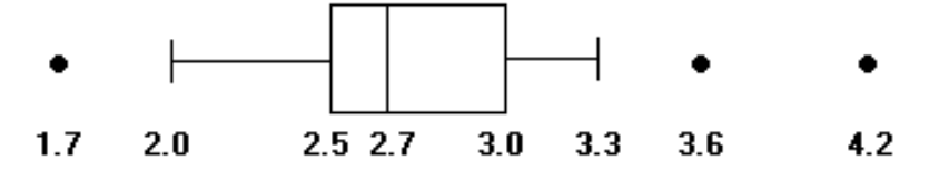
Construct a modified boxplot for the data. Identify any outliers.
-The weights (in ounces) of 27 tomatoes are listed below.
A) Outliers: 1.7 oz, 4.2 oz
B) No outliers
C) Outlier: 4.2 oz
D) Outliers: 1.7 oz, 3.6 oz, 4.2 oz
-The weights (in ounces) of 27 tomatoes are listed below.
A) Outliers: 1.7 oz, 4.2 oz
B) No outliers
C) Outlier: 4.2 oz
D) Outliers: 1.7 oz, 3.6 oz, 4.2 oz
Unlock Deck
Unlock for access to all 187 flashcards in this deck.
Unlock Deck
k this deck
77
The ages of the members of a gym have a mean of 48 years and a standard deviation of 10 years. What can you conclude from Chebyshev's theorem about the percentage of gym members aged between 26 and 70?
A) The percentage is at least 79.3%
B) The percentage is approximately 54.5%
C) The percentage is at least 54.5%
D) The percentage is at most 79.3%
A) The percentage is at least 79.3%
B) The percentage is approximately 54.5%
C) The percentage is at least 54.5%
D) The percentage is at most 79.3%
Unlock Deck
Unlock for access to all 187 flashcards in this deck.
Unlock Deck
k this deck
78
Find the mean for the given sample data. Unless indicated otherwise, round your answer to one more decimal place than is present in the original data values.
-Listed below are the amounts of time (in months) that the employees of a restaurant have been working at the restaurant. Find the mean.
A) 21.5 months
B) 54.4 months
C) 58.5 months
D) 50.7 months
-Listed below are the amounts of time (in months) that the employees of a restaurant have been working at the restaurant. Find the mean.
A) 21.5 months
B) 54.4 months
C) 58.5 months
D) 50.7 months
Unlock Deck
Unlock for access to all 187 flashcards in this deck.
Unlock Deck
k this deck
79
Find the mode(s) for the given sample data.
-
A) 80
B) 80, 46
C) 46
D) 52.2
-
A) 80
B) 80, 46
C) 46
D) 52.2
Unlock Deck
Unlock for access to all 187 flashcards in this deck.
Unlock Deck
k this deck
80
Find the midrange for the given sample data.
-The speeds (in mph) of the cars passing a certain checkpoint are measured by radar. The results are shown below. Find the midrange.
A) 4.80 mph
B) 42.2 mph
C) 42.60 mph
D) 42.15 mph
-The speeds (in mph) of the cars passing a certain checkpoint are measured by radar. The results are shown below. Find the midrange.
A) 4.80 mph
B) 42.2 mph
C) 42.60 mph
D) 42.15 mph
Unlock Deck
Unlock for access to all 187 flashcards in this deck.
Unlock Deck
k this deck
Unlock Deck
Unlock for access to all 187 flashcards in this deck.


