Deck 4: Regression Analysis: Exploring Associations Between Variables
Full screen (f)
Question
Use the following information for following questions .
The following scatterplot shows the relationship between heights (in cm) and weights (in kg) of 100
Americans. The coefficient of determination was found to be 37.9%.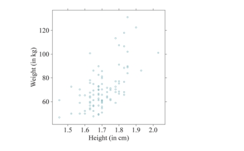
Calculate the value of the correlation coefficient between height and weight.
The following scatterplot shows the relationship between heights (in cm) and weights (in kg) of 100
Americans. The coefficient of determination was found to be 37.9%.
Calculate the value of the correlation coefficient between height and weight.
Question
Use the following regression equation regarding airline tickets for following questions .  Note that Distance is the amount of miles between the departure and arrival cities, and Price is the
cost of an airline ticket.
Interpret the slope of the regression equation in the context of the data.
Note that Distance is the amount of miles between the departure and arrival cities, and Price is thecost of an airline ticket.
Interpret the slope of the regression equation in the context of the data.
Question
Use the following regression equation regarding airline tickets for following questions . Note that Distance is the amount of miles between the departure and arrival cities, and Price is the
cost of an airline ticket.
What is the expected ticket price for a flight between Los Angeles and New York City, which are 2448.3 miles apart?
Note that Distance is the amount of miles between the departure and arrival cities, and Price is thecost of an airline ticket.
What is the expected ticket price for a flight between Los Angeles and New York City, which are 2448.3 miles apart?
Question
Which of the following scatterplots shows data with the highest correlation between the explanatory and response variables? Explain your reasoning. 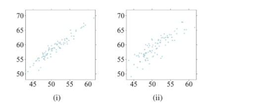
Question
For the following scatterplot, what effect would the outlier have on the slope of the regression equation? Explain your reasoning. 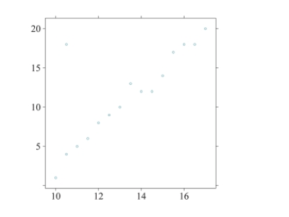
Question
Given the following scatterplot, if the point in the upper left corner were removed, what would happen to the value of the correlation coefficient, r? 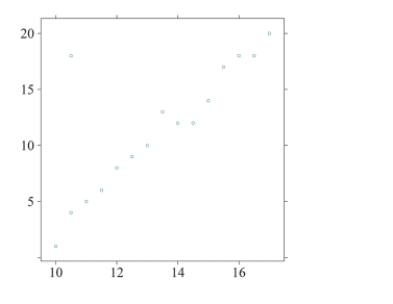
Question
Use the following information to answer Questions .
The scatterplot below shows the relationship between the average monthly temperature and the
monthly cost of a gas bill. The correlation coefficient between the values is −0.92.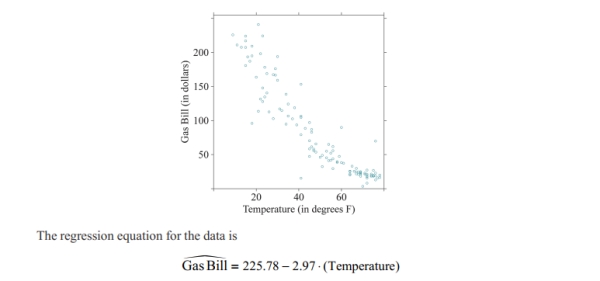
Do lower monthly temperature cause gas bills to be more expensive? Explain your reasoning.
The scatterplot below shows the relationship between the average monthly temperature and the
monthly cost of a gas bill. The correlation coefficient between the values is −0.92.
Do lower monthly temperature cause gas bills to be more expensive? Explain your reasoning.
Question
Question
Question
Question
Question
Use the following information for following questions .
The following scatterplot shows the relationship between heights (in cm) and weights (in kg) of 100
Americans. The coefficient of determination was found to be 37.9%.
If we converted the x- axis to inches, instead of centimeters, what would happen to the value of the correlation coefficient?
The following scatterplot shows the relationship between heights (in cm) and weights (in kg) of 100
Americans. The coefficient of determination was found to be 37.9%.
If we converted the x- axis to inches, instead of centimeters, what would happen to the value of the correlation coefficient?
Question
Use the following information to answer Questions .
The scatterplot below shows the relationship between the average monthly temperature and the
monthly cost of a gas bill. The correlation coefficient between the values is −0.92.
Determine the value of the coefficient of determination and explain its meaning in context?
The scatterplot below shows the relationship between the average monthly temperature and the
monthly cost of a gas bill. The correlation coefficient between the values is −0.92.
Determine the value of the coefficient of determination
and explain its meaning in context? Question
Use the following regression equation regarding airline tickets for following questions . Note that Distance is the amount of miles between the departure and arrival cities, and Price is the
cost of an airline ticket.
Interpret the intercept of the regression equation in the context of the data. Explain why the value is or is not meaningful.
Note that Distance is the amount of miles between the departure and arrival cities, and Price is thecost of an airline ticket.
Interpret the intercept of the regression equation in the context of the data. Explain why the value is or is not meaningful.
Question
Which scatterplot below depicts a stronger linear relationship? Why? Explain what the scatterplot shows regarding a tree's volume. 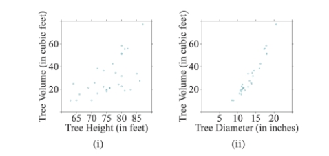
Question
Question
Question
Question
Question
Use the following information to answer Questions .
The scatterplot below shows the relationship between the average monthly temperature and the
monthly cost of a gas bill. The correlation coefficient between the values is −0.92.
If appropriate, calculate the expected gas bill cost for a month with an average temperature of − . If it's not appropriate, explain why.
The scatterplot below shows the relationship between the average monthly temperature and the
monthly cost of a gas bill. The correlation coefficient between the values is −0.92.
If appropriate, calculate the expected gas bill cost for a month with an average temperature of −
. If it's not appropriate, explain why. Question
Use the following information for following questions .
The scatterplot shows the relationship between the foot lengths and foot widths of children. The
coefficient of determination was found to be 41.09%.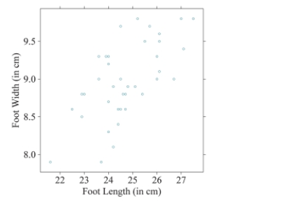
If we converted the x-axis to inches, instead of centimeters, what would happen to the value of the correlation coefficient?
A)The correlation coefficient would increase because we there are 2.54 centimeters in 1 inch.
B)The correlation coefficient would decrease because we there are 2.54 centimeters in 1 inch.
C)The correlation coefficient would be unchanged because it is not affected by changes in units.
D)We cannot make any conclusions about the correlation coefficient because we would need to use the new data values (with inches) to calculate it.
Question
Which of the following sets of numbers would result in a positive correlation of 1?
A)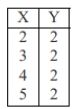
B)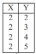
C)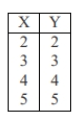
D)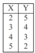
A)
B)
C)
D)
Question
Given the following scatterplot, if a point was added in the upper left corner with an x-value of 10 and a y-value of 20, what would happen to the value of the correlation coefficient, r? 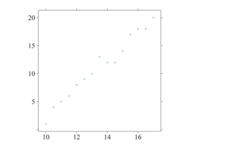
A)r will get closer to 0.
B)r will get closer to 1.
C)r will get closer to -1.
D)r will not change.
A)r will get closer to 0.
B)r will get closer to 1.
C)r will get closer to -1.
D)r will not change.
Question
Use the following regression equation regarding car mileage for following questions .  Note that City is the estimated miles per gallon (mpg) a car gets while driving on city streets, and
Highway is the estimated miles per gallon (mpg) a car gets while driving on highways.
Interpret the slope in the context of the data.
A)The slope is 0.892.For every additional mpg a car gets in the city, its highway mpg is predicted to increase by 0.892.
B)The slope is 1.337.For every additional mpg a car gets in the city, its highway mpg is predicted to increase by 1.337.
C)The slope is 0.892.If a car gets 0 mpg in the city, it will get 0.892 mpg on the highway.
D)The slope is 1.337.If a car gets 0 mpg in the city, it will get 1.337 mpg on the highway.
Note that City is the estimated miles per gallon (mpg) a car gets while driving on city streets, andHighway is the estimated miles per gallon (mpg) a car gets while driving on highways.
Interpret the slope in the context of the data.
A)The slope is 0.892.For every additional mpg a car gets in the city, its highway mpg is predicted to increase by 0.892.
B)The slope is 1.337.For every additional mpg a car gets in the city, its highway mpg is predicted to increase by 1.337.
C)The slope is 0.892.If a car gets 0 mpg in the city, it will get 0.892 mpg on the highway.
D)The slope is 1.337.If a car gets 0 mpg in the city, it will get 1.337 mpg on the highway.
Question
Question
Question
Use the following information for following questions .
The scatterplot shows the relationship between the foot lengths and foot widths of children. The
coefficient of determination was found to be 41.09%.
Calculate the value of the correlation coefficient between a car's age and its current value.
A)r =−0.4109
B)r =−0.6410
C)r = 0.4109
D)r = 0.6410
The scatterplot shows the relationship between the foot lengths and foot widths of children. The
coefficient of determination was found to be 41.09%.
Calculate the value of the correlation coefficient between a car's age and its current value.
A)r =−0.4109
B)r =−0.6410
C)r = 0.4109
D)r = 0.6410
Question
Question
Use the following information to answer Questions .
The scatterplot below shows the relationship between a car's speed and the distance it traveled to come
to a complete stop when hitting the brakes. The correlation coefficient between the values is 0.81.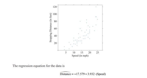
Would it be appropriate to say that a car's speed causes its stopping distance?
A)Yes, the scatterplot shows a strong linear association, so the faster a car is going, the longer it takes to stop it.
B)Yes, since the correlation coefficient is close to 1, we can conclude causation.
C)No, since the correlation coefficient does not equal 1, we cannot conclude causation.
D)No, correlation never implies causation.
Question
Use the following regression equation regarding car mileage for following questions . Note that City is the estimated miles per gallon (mpg) a car gets while driving on city streets, and
Highway is the estimated miles per gallon (mpg) a car gets while driving on highways.
Interpret the intercept in the context of the data. State whether the value is meaningful.
A)The intercept is 0.892.For every additional mpg a car gets in the city, its highway mpg is predicted to increase by 0.892.The value is meaningful.
B)The intercept is 1.337.For every additional mpg a car gets in the city, its highway mpg is predicted to increase by 1.337.The value is meaningful.
C)The intercept is 0.892.If a car gets 0 mpg in the city, it will get 0.892 mpg on the highway. The value is not meaningful because if a car is not moving, it cannot have a mpg value.
D)The intercept is 1.337.If a car gets 0 mpg in the city, it will get 1.337 mpg on the highway. The value is not meaningful because if a car is not moving, it cannot have a mpg value.
Note that City is the estimated miles per gallon (mpg) a car gets while driving on city streets, andHighway is the estimated miles per gallon (mpg) a car gets while driving on highways.
Interpret the intercept in the context of the data. State whether the value is meaningful.
A)The intercept is 0.892.For every additional mpg a car gets in the city, its highway mpg is predicted to increase by 0.892.The value is meaningful.
B)The intercept is 1.337.For every additional mpg a car gets in the city, its highway mpg is predicted to increase by 1.337.The value is meaningful.
C)The intercept is 0.892.If a car gets 0 mpg in the city, it will get 0.892 mpg on the highway. The value is not meaningful because if a car is not moving, it cannot have a mpg value.
D)The intercept is 1.337.If a car gets 0 mpg in the city, it will get 1.337 mpg on the highway. The value is not meaningful because if a car is not moving, it cannot have a mpg value.
Question
Use the following information to answer Questions .
The scatterplot below shows the relationship between a car's speed and the distance it traveled to come
to a complete stop when hitting the brakes. The correlation coefficient between the values is 0.81.
[Objective: Interpret the coefficient of determination in context.] What is the value of the coefficient of determination![<strong>Use the following information to answer Questions . The scatterplot below shows the relationship between a car's speed and the distance it traveled to come to a complete stop when hitting the brakes. The correlation coefficient between the values is 0.81. [Objective: Interpret the coefficient of determination in context.] What is the value of the coefficient of determination and what does it mean in context?</strong> A) B) C) D) <div style=padding-top: 35px>](https://d2lvgg3v3hfg70.cloudfront.net/TB34225555/11ec8f09_0947_2daa_aaa3_2bb95a6feab0_TB34225555_11.jpg) and what does it mean in context?
and what does it mean in context?
A)![<strong>Use the following information to answer Questions . The scatterplot below shows the relationship between a car's speed and the distance it traveled to come to a complete stop when hitting the brakes. The correlation coefficient between the values is 0.81. [Objective: Interpret the coefficient of determination in context.] What is the value of the coefficient of determination and what does it mean in context?</strong> A) B) C) D) <div style=padding-top: 35px>](https://d2lvgg3v3hfg70.cloudfront.net/TB34225555/11ec8f09_0948_180b_aaa3_f7e24b2f92e8_TB34225555_11.jpg)
B)![<strong>Use the following information to answer Questions . The scatterplot below shows the relationship between a car's speed and the distance it traveled to come to a complete stop when hitting the brakes. The correlation coefficient between the values is 0.81. [Objective: Interpret the coefficient of determination in context.] What is the value of the coefficient of determination and what does it mean in context?</strong> A) B) C) D) <div style=padding-top: 35px>](https://d2lvgg3v3hfg70.cloudfront.net/TB34225555/11ec8f09_094b_254c_aaa3_f17dbf68fe9d_TB34225555_11.jpg)
C)![<strong>Use the following information to answer Questions . The scatterplot below shows the relationship between a car's speed and the distance it traveled to come to a complete stop when hitting the brakes. The correlation coefficient between the values is 0.81. [Objective: Interpret the coefficient of determination in context.] What is the value of the coefficient of determination and what does it mean in context?</strong> A) B) C) D) <div style=padding-top: 35px>](https://d2lvgg3v3hfg70.cloudfront.net/TB34225555/11ec8f09_094d_6f3d_aaa3_cf0e7379abd2_TB34225555_11.jpg)
D)![<strong>Use the following information to answer Questions . The scatterplot below shows the relationship between a car's speed and the distance it traveled to come to a complete stop when hitting the brakes. The correlation coefficient between the values is 0.81. [Objective: Interpret the coefficient of determination in context.] What is the value of the coefficient of determination and what does it mean in context?</strong> A) B) C) D) <div style=padding-top: 35px>](https://d2lvgg3v3hfg70.cloudfront.net/TB34225555/11ec8f09_094f_6b0e_aaa3_6783e2d1c11a_TB34225555_11.jpg)
The scatterplot below shows the relationship between a car's speed and the distance it traveled to come
to a complete stop when hitting the brakes. The correlation coefficient between the values is 0.81.
[Objective: Interpret the coefficient of determination in context.] What is the value of the coefficient of determination
and what does it mean in context?A)
B)
C)
D)
Question
Use the following information for following questions .
Data were recorded for 117 months on a household's gas bill (in dollars) and the average monthly temperatures for its neighborhood. The mean monthly temperature was 48.7° F with a standard deviation of 20.6. The mean gas bill price was $81.20 with a standard deviation of 66.5. The correlation coefficient between monthly temperature and gas bill price is −0.92.
Determine which is the correct calculation of the intercept for the linear model that predicts gas bill price from monthly temperature.
A)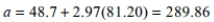
B)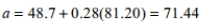
C)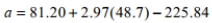
D)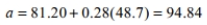
Question
Question
Question
Use the following information to answer Questions .
The scatterplot below shows the relationship between a car's speed and the distance it traveled to come
to a complete stop when hitting the brakes. The correlation coefficient between the values is 0.81.
Can we use the regression equation to predict the stopping distance of a car that is traveling at 40 mph?
A)No, we cannot make a prediction because a car that is traveling at 40 mph is outside the range of our data.We would be extrapolating.
B)No, we cannot make a prediction because the correlation coefficient does not equal 1.
C)Yes, we can always make predictions once we have a regression equation.
D)Yes, we can make a prediction because the scatterplot shows a strong positive linear relationship.
Question
Use the following regression equation regarding car mileage for following questions . Note that City is the estimated miles per gallon (mpg) a car gets while driving on city streets, and
Highway is the estimated miles per gallon (mpg) a car gets while driving on highways.
What is the expected highway mpg for a car that gets 23 mpg in cities?
A)16.5 mpg
B)21.9 mpg
C)30.8 mpg
D)31.6 mpg
Note that City is the estimated miles per gallon (mpg) a car gets while driving on city streets, andHighway is the estimated miles per gallon (mpg) a car gets while driving on highways.
What is the expected highway mpg for a car that gets 23 mpg in cities?
A)16.5 mpg
B)21.9 mpg
C)30.8 mpg
D)31.6 mpg
Question
Which scatterplot below depicts a stronger linear relationship? Why? 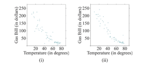
A)Scatterplot (i) shows a stronger linear relationship because it has less vertical variation between points.
B)Scatterplot (i) shows a stronger linear relationship because it has more vertical variation between points.
C)Scatterplot (ii) shows a stronger linear relationship because it has less vertical variation between points.
D)Scatterplot (ii) shows a stronger linear relationship because it has more vertical variation between points.
Question
Question
Question
Which of the following scatterplots shows data with the highest correlation between the explanatory and response variables?
A)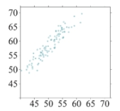
B)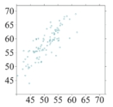
C)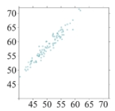
D)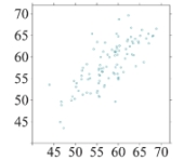
A)
B)
C)
D)
Question
Given the following scatterplot, if the point in the upper right corner were removed, what will happen to the value of the correlation coefficient, r? 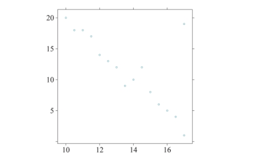
A)r will get closer to 1.
B)r will get closer to 0.
C)r will get closer to −1.
D)r will not change.
A)r will get closer to 1.
B)r will get closer to 0.
C)r will get closer to −1.
D)r will not change.
Question
Question
Which of the following sets of numbers would result in a negative correlation of −1?
A)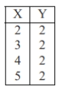
B)
C)
D)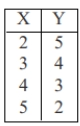
A)
B)
C)
D)
Question
Question
Use the following regression equation regarding professor salaries for following questions .  )
)
Note that Years is the number of years a professor has worked at a college, and Salary is the annual
salary (in dollars) the professor earns.
Interpret the slope in the context of the data.
A)The slope is 1280.If a professor has never worked at a college, his/her salary is expected to be $1,280.
B)The slope is 95000.If a professor has never worked at a college, his/her salary is expected to be $95,000.
C)The slope is 1280.For every additional year a professor works at a college, his/her salary is predicted to increase by $1,280.
D)The slope is 95000.For every additional year a professor works at a college, his/her salary is predicted to increase by $95,000.
)Note that Years is the number of years a professor has worked at a college, and Salary is the annual
salary (in dollars) the professor earns.
Interpret the slope in the context of the data.
A)The slope is 1280.If a professor has never worked at a college, his/her salary is expected to be $1,280.
B)The slope is 95000.If a professor has never worked at a college, his/her salary is expected to be $95,000.
C)The slope is 1280.For every additional year a professor works at a college, his/her salary is predicted to increase by $1,280.
D)The slope is 95000.For every additional year a professor works at a college, his/her salary is predicted to increase by $95,000.
Question
Question
Question
Use the following information for following questions
The scatterplot shows the relationship between a vehicle's age (in years) and its current value (in
dollars). The coefficient of determination was found to be 98.74%.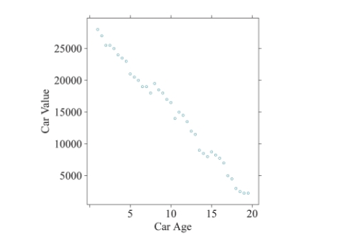
If we converted the x-axis to months, instead of years, what would happen to the value of the correlation coefficient?
A)The correlation coefficient would increase because we are adding 12 additional values (one for each month) on the x-axis.
B)The correlation coefficient would decrease because we have less data points per month as opposed to per year.
C)The correlation coefficient would be unchanged because it is not affected by changes in units.
D)We cannot make any conclusions about the correlation coefficient because we would need to use the new data values to calculate it.
Question
[Objective: Determine the effects of outliers on a regression equation.] What effects might an outlier have on a regression equation?
A) An outlier has no effect on a regression equation.
B) An outlier may affect only the slope of a regression equation.
C) An outlier may affect only the correlation coefficient of a regression equation.
D) An outlier may affect both the slope and the correlation coefficient of a regression equation.
Use the following information to answer Questions (15) and (16).
The scatterplot below shows the relationship between the ages of women when they first married and the ages when they had their first child. The correlation coefficient between the values is 0.9315.
![<strong>[Objective: Determine the effects of outliers on a regression equation.] What effects might an outlier have on a regression equation? </strong> A) An outlier has no effect on a regression equation. B) An outlier may affect only the slope of a regression equation. C) An outlier may affect only the correlation coefficient of a regression equation. D) An outlier may affect both the slope and the correlation coefficient of a regression equation. Use the following information to answer Questions (15) and (16). The scatterplot below shows the relationship between the ages of women when they first married and the ages when they had their first child. The correlation coefficient between the values is 0.9315. <div style=padding-top: 35px>](https://d2lvgg3v3hfg70.cloudfront.net/TB3889/11eb4848_5bfe_9c0c_bdae_c1edc0fa5df7_TB3889_00.jpg)
A) An outlier has no effect on a regression equation.
B) An outlier may affect only the slope of a regression equation.
C) An outlier may affect only the correlation coefficient of a regression equation.
D) An outlier may affect both the slope and the correlation coefficient of a regression equation.
Use the following information to answer Questions (15) and (16).
The scatterplot below shows the relationship between the ages of women when they first married and the ages when they had their first child. The correlation coefficient between the values is 0.9315.
Question
Question
Question
Question
Which scatterplot below depicts a stronger linear relationship? Why? 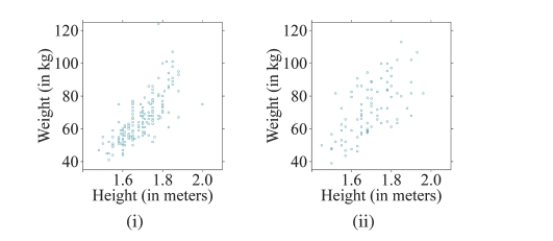
A)Scatterplot (i) shows a stronger linear relationship because it has less vertical variation between points.
B)Scatterplot (i) shows a stronger linear relationship because it has more vertical variation between points.
C)Scatterplot (ii) shows a stronger linear relationship because it has less vertical variation between points.
D)Scatterplot (ii) shows a stronger linear relationship because it has more vertical variation between points.
A)Scatterplot (i) shows a stronger linear relationship because it has less vertical variation between points.
B)Scatterplot (i) shows a stronger linear relationship because it has more vertical variation between points.
C)Scatterplot (ii) shows a stronger linear relationship because it has less vertical variation between points.
D)Scatterplot (ii) shows a stronger linear relationship because it has more vertical variation between points.
Question
Which of the following scatterplots shows data with the highest correlation between the explanatory and response variables?
A)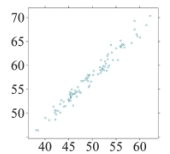
B)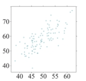
C)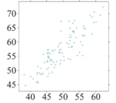
D)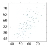
A)
B)
C)
D)
Question
Question
Use the following information for following questions
The scatterplot shows the relationship between a vehicle's age (in years) and its current value (in
dollars). The coefficient of determination was found to be 98.74%.
Calculate the value of the correlation coefficient between a car's age and its current value.
A)r = 0.9937
B)r = 0.9874
C)r =−0.9937
D)r =−0.9874
Question
Use the following regression equation regarding professor salaries for following questions . )
Note that Years is the number of years a professor has worked at a college, and Salary is the annual
salary (in dollars) the professor earns.
What is the expected salary of a professor who has worked at a college for 15 years?
A)$95,000
B)$96,280
C)$106,700
D)$114,200
)Note that Years is the number of years a professor has worked at a college, and Salary is the annual
salary (in dollars) the professor earns.
What is the expected salary of a professor who has worked at a college for 15 years?
A)$95,000
B)$96,280
C)$106,700
D)$114,200
Question
Question
[Objective: Interpret the coefficient of determination in context.] Suppose the correlation coefficient describing how the heights of teenage boys predicts their weights is 0.85. What is the coefficient of determination ![<strong>[Objective: Interpret the coefficient of determination in context.] Suppose the correlation coefficient describing how the heights of teenage boys predicts their weights is 0.85. What is the coefficient of determination and what does it mean in context?</strong> A) of the variation in heights of teenage boys can be explained by their weight. B) of the variation in weights of teenage boys can be explained by their height. C) is 0.85 .85% of the variation in heights of teenage boys can be explained by their weight. d. is 0.85 .85% of the variation in weights of teenage boys can be explained by their height. <div style=padding-top: 35px>](https://d2lvgg3v3hfg70.cloudfront.net/TB34225555/11ec8f0a_6796_be77_aaa3_e9c3113eb5a7_TB34225555_11.jpg) and what does it mean in context?
and what does it mean in context?
A)![<strong>[Objective: Interpret the coefficient of determination in context.] Suppose the correlation coefficient describing how the heights of teenage boys predicts their weights is 0.85. What is the coefficient of determination and what does it mean in context?</strong> A) of the variation in heights of teenage boys can be explained by their weight. B) of the variation in weights of teenage boys can be explained by their height. C) is 0.85 .85% of the variation in heights of teenage boys can be explained by their weight. d. is 0.85 .85% of the variation in weights of teenage boys can be explained by their height. <div style=padding-top: 35px>](https://d2lvgg3v3hfg70.cloudfront.net/TB34225555/11ec8f0a_6797_cfe8_aaa3_a7a984687e22_TB34225555_11.jpg) of the variation in heights of teenage boys can be explained by their weight.
of the variation in heights of teenage boys can be explained by their weight.
B)![<strong>[Objective: Interpret the coefficient of determination in context.] Suppose the correlation coefficient describing how the heights of teenage boys predicts their weights is 0.85. What is the coefficient of determination and what does it mean in context?</strong> A) of the variation in heights of teenage boys can be explained by their weight. B) of the variation in weights of teenage boys can be explained by their height. C) is 0.85 .85% of the variation in heights of teenage boys can be explained by their weight. d. is 0.85 .85% of the variation in weights of teenage boys can be explained by their height. <div style=padding-top: 35px>](https://d2lvgg3v3hfg70.cloudfront.net/TB34225555/11ec8f0a_6798_ba49_aaa3_0b52739b0abe_TB34225555_11.jpg) of the variation in weights of teenage boys can be explained by their height.
of the variation in weights of teenage boys can be explained by their height.
C)![<strong>[Objective: Interpret the coefficient of determination in context.] Suppose the correlation coefficient describing how the heights of teenage boys predicts their weights is 0.85. What is the coefficient of determination and what does it mean in context?</strong> A) of the variation in heights of teenage boys can be explained by their weight. B) of the variation in weights of teenage boys can be explained by their height. C) is 0.85 .85% of the variation in heights of teenage boys can be explained by their weight. d. is 0.85 .85% of the variation in weights of teenage boys can be explained by their height. <div style=padding-top: 35px>](https://d2lvgg3v3hfg70.cloudfront.net/TB34225555/11ec8f0a_6799_7d9a_aaa3_fbdc28f26d31_TB34225555_11.jpg) is 0.85 .85% of the variation in heights of teenage boys can be explained by their weight. d.
is 0.85 .85% of the variation in heights of teenage boys can be explained by their weight. d. ![<strong>[Objective: Interpret the coefficient of determination in context.] Suppose the correlation coefficient describing how the heights of teenage boys predicts their weights is 0.85. What is the coefficient of determination and what does it mean in context?</strong> A) of the variation in heights of teenage boys can be explained by their weight. B) of the variation in weights of teenage boys can be explained by their height. C) is 0.85 .85% of the variation in heights of teenage boys can be explained by their weight. d. is 0.85 .85% of the variation in weights of teenage boys can be explained by their height. <div style=padding-top: 35px>](https://d2lvgg3v3hfg70.cloudfront.net/TB34225555/11ec8f0a_6799_cbbb_aaa3_3195dbe9ad6c_TB34225555_11.jpg) is 0.85 .85% of the variation in weights of teenage boys can be explained by their height.
is 0.85 .85% of the variation in weights of teenage boys can be explained by their height.
and what does it mean in context?A)
of the variation in heights of teenage boys can be explained by their weight.B)
of the variation in weights of teenage boys can be explained by their height.C)
is 0.85 .85% of the variation in heights of teenage boys can be explained by their weight. d. is 0.85 .85% of the variation in weights of teenage boys can be explained by their height.
Unlock Deck
Sign up to unlock the cards in this deck!
Unlock Deck
Unlock Deck
1/59
Play
Full screen (f)
Deck 4: Regression Analysis: Exploring Associations Between Variables
1
Use the following information for following questions .
The following scatterplot shows the relationship between heights (in cm) and weights (in kg) of 100
Americans. The coefficient of determination was found to be 37.9%.
Calculate the value of the correlation coefficient between height and weight.
The following scatterplot shows the relationship between heights (in cm) and weights (in kg) of 100
Americans. The coefficient of determination was found to be 37.9%.
Calculate the value of the correlation coefficient between height and weight.
2
Use the following regression equation regarding airline tickets for following questions . Note that Distance is the amount of miles between the departure and arrival cities, and Price is the
cost of an airline ticket.
Interpret the slope of the regression equation in the context of the data.
Note that Distance is the amount of miles between the departure and arrival cities, and Price is thecost of an airline ticket.
Interpret the slope of the regression equation in the context of the data.
The slope is 0.22. For every additional mile of flight travel, the price of the airline ticket is predicted to increase by $0.22.
3
Use the following regression equation regarding airline tickets for following questions . Note that Distance is the amount of miles between the departure and arrival cities, and Price is the
cost of an airline ticket.
What is the expected ticket price for a flight between Los Angeles and New York City, which are 2448.3 miles apart?
Note that Distance is the amount of miles between the departure and arrival cities, and Price is thecost of an airline ticket.
What is the expected ticket price for a flight between Los Angeles and New York City, which are 2448.3 miles apart?

4
Which of the following scatterplots shows data with the highest correlation between the explanatory and response variables? Explain your reasoning.
Unlock Deck
Unlock for access to all 59 flashcards in this deck.
Unlock Deck
k this deck
5
For the following scatterplot, what effect would the outlier have on the slope of the regression equation? Explain your reasoning.
Unlock Deck
Unlock for access to all 59 flashcards in this deck.
Unlock Deck
k this deck
6
Given the following scatterplot, if the point in the upper left corner were removed, what would happen to the value of the correlation coefficient, r?
Unlock Deck
Unlock for access to all 59 flashcards in this deck.
Unlock Deck
k this deck
7
Use the following information to answer Questions .
The scatterplot below shows the relationship between the average monthly temperature and the
monthly cost of a gas bill. The correlation coefficient between the values is −0.92.
Do lower monthly temperature cause gas bills to be more expensive? Explain your reasoning.
The scatterplot below shows the relationship between the average monthly temperature and the
monthly cost of a gas bill. The correlation coefficient between the values is −0.92.
Do lower monthly temperature cause gas bills to be more expensive? Explain your reasoning.
Unlock Deck
Unlock for access to all 59 flashcards in this deck.
Unlock Deck
k this deck
8
A study about exercise routines reported that the amount of time a person spends working out has a strong positive linear association with the amount of weight he/she loses. What can you determine about the relationship between amount of time spent at the gym and the amount of weight a person loses?
Unlock Deck
Unlock for access to all 59 flashcards in this deck.
Unlock Deck
k this deck
9
Use the following information for following questions .
Suppose data were recorded for 100 employees of a large company that included annual salaries
and the number of years the employee has been in their current position. The mean annual salary
was $58,000 with a standard deviation of 12,500. The mean number of years in the current
position is 10 with a standard deviation of 3. The correlation coefficient between the two
variables is approximately 0.93.
Calculation the value of the intercept for the linear model that predicts annual salary from the number of years in current position and interpret it in context, if appropriate.
Unlock Deck
Unlock for access to all 59 flashcards in this deck.
Unlock Deck
k this deck
10
When will a correlation coefficient be negative?
Unlock Deck
Unlock for access to all 59 flashcards in this deck.
Unlock Deck
k this deck
11
Use the following information for following questions .
Suppose data were recorded for 100 employees of a large company that included annual salaries
and the number of years the employee has been in their current position. The mean annual salary
was $58,000 with a standard deviation of 12,500. The mean number of years in the current
position is 10 with a standard deviation of 3. The correlation coefficient between the two
variables is approximately 0.93.
Determine the correct value of the slope for the linear model that predicts annual salary from the number of years in current position and interpret it in context.
Unlock Deck
Unlock for access to all 59 flashcards in this deck.
Unlock Deck
k this deck
12
Use the following information for following questions .
The following scatterplot shows the relationship between heights (in cm) and weights (in kg) of 100
Americans. The coefficient of determination was found to be 37.9%.
If we converted the x- axis to inches, instead of centimeters, what would happen to the value of the correlation coefficient?
The following scatterplot shows the relationship between heights (in cm) and weights (in kg) of 100
Americans. The coefficient of determination was found to be 37.9%.
If we converted the x- axis to inches, instead of centimeters, what would happen to the value of the correlation coefficient?
Unlock Deck
Unlock for access to all 59 flashcards in this deck.
Unlock Deck
k this deck
13
Use the following information to answer Questions .
The scatterplot below shows the relationship between the average monthly temperature and the
monthly cost of a gas bill. The correlation coefficient between the values is −0.92.
Determine the value of the coefficient of determination and explain its meaning in context?
The scatterplot below shows the relationship between the average monthly temperature and the
monthly cost of a gas bill. The correlation coefficient between the values is −0.92.
Determine the value of the coefficient of determination
and explain its meaning in context? Unlock Deck
Unlock for access to all 59 flashcards in this deck.
Unlock Deck
k this deck
14
Use the following regression equation regarding airline tickets for following questions . Note that Distance is the amount of miles between the departure and arrival cities, and Price is the
cost of an airline ticket.
Interpret the intercept of the regression equation in the context of the data. Explain why the value is or is not meaningful.
Note that Distance is the amount of miles between the departure and arrival cities, and Price is thecost of an airline ticket.
Interpret the intercept of the regression equation in the context of the data. Explain why the value is or is not meaningful.
Unlock Deck
Unlock for access to all 59 flashcards in this deck.
Unlock Deck
k this deck
15
Which scatterplot below depicts a stronger linear relationship? Why? Explain what the scatterplot shows regarding a tree's volume.
Unlock Deck
Unlock for access to all 59 flashcards in this deck.
Unlock Deck
k this deck
16
Use the following information for following questions .
Suppose data were recorded for 100 employees of a large company that included annual salaries
and the number of years the employee has been in their current position. The mean annual salary
was $58,000 with a standard deviation of 12,500. The mean number of years in the current
position is 10 with a standard deviation of 3. The correlation coefficient between the two
variables is approximately 0.93.
If an employee earns an annual salary of $85,000, approximately how long has she held her current position at the company? Round your answer to the nearest year.
Unlock Deck
Unlock for access to all 59 flashcards in this deck.
Unlock Deck
k this deck
17
Suppose the heights of teenagers were recorded in 2003 and then recorded again 5 years later, in 2008. For each person, the height in 2008 was 6 inches (15.24 centimeters) taller than the height in 2003. For example, a teenager who was 53 inches (134.62 cm) tall in 2003 measured at a height of 59 inches (149.86 cm) in 2008. What would be the correlation coefficient between the 2003 heights and the 2008 heights? Explain your reasoning.
Unlock Deck
Unlock for access to all 59 flashcards in this deck.
Unlock Deck
k this deck
18
Suppose data were collected on neighborhoods about the number of crimes committed and the number of police who patrol the area. Which variable is the explanatory variable and which one is the response? Ex- plain your reasoning.
Unlock Deck
Unlock for access to all 59 flashcards in this deck.
Unlock Deck
k this deck
19
Create a data set of 2 variables (X and Y) such that the relationship between X and Y would have a perfect negative correlation of −1.Note: The data set can be very small (three to four X and Y values).
Unlock Deck
Unlock for access to all 59 flashcards in this deck.
Unlock Deck
k this deck
20
Use the following information to answer Questions .
The scatterplot below shows the relationship between the average monthly temperature and the
monthly cost of a gas bill. The correlation coefficient between the values is −0.92.
If appropriate, calculate the expected gas bill cost for a month with an average temperature of − . If it's not appropriate, explain why.
The scatterplot below shows the relationship between the average monthly temperature and the
monthly cost of a gas bill. The correlation coefficient between the values is −0.92.
If appropriate, calculate the expected gas bill cost for a month with an average temperature of −
. If it's not appropriate, explain why. Unlock Deck
Unlock for access to all 59 flashcards in this deck.
Unlock Deck
k this deck
21
Use the following information for following questions .
The scatterplot shows the relationship between the foot lengths and foot widths of children. The
coefficient of determination was found to be 41.09%.
If we converted the x-axis to inches, instead of centimeters, what would happen to the value of the correlation coefficient?
A)The correlation coefficient would increase because we there are 2.54 centimeters in 1 inch.
B)The correlation coefficient would decrease because we there are 2.54 centimeters in 1 inch.
C)The correlation coefficient would be unchanged because it is not affected by changes in units.
D)We cannot make any conclusions about the correlation coefficient because we would need to use the new data values (with inches) to calculate it.
Unlock Deck
Unlock for access to all 59 flashcards in this deck.
Unlock Deck
k this deck
22
Which of the following sets of numbers would result in a positive correlation of 1?
A)
B)
C)
D)
A)
B)
C)
D)
Unlock Deck
Unlock for access to all 59 flashcards in this deck.
Unlock Deck
k this deck
23
Given the following scatterplot, if a point was added in the upper left corner with an x-value of 10 and a y-value of 20, what would happen to the value of the correlation coefficient, r?
A)r will get closer to 0.
B)r will get closer to 1.
C)r will get closer to -1.
D)r will not change.
A)r will get closer to 0.
B)r will get closer to 1.
C)r will get closer to -1.
D)r will not change.
Unlock Deck
Unlock for access to all 59 flashcards in this deck.
Unlock Deck
k this deck
24
Use the following regression equation regarding car mileage for following questions . Note that City is the estimated miles per gallon (mpg) a car gets while driving on city streets, and
Highway is the estimated miles per gallon (mpg) a car gets while driving on highways.
Interpret the slope in the context of the data.
A)The slope is 0.892.For every additional mpg a car gets in the city, its highway mpg is predicted to increase by 0.892.
B)The slope is 1.337.For every additional mpg a car gets in the city, its highway mpg is predicted to increase by 1.337.
C)The slope is 0.892.If a car gets 0 mpg in the city, it will get 0.892 mpg on the highway.
D)The slope is 1.337.If a car gets 0 mpg in the city, it will get 1.337 mpg on the highway.
Note that City is the estimated miles per gallon (mpg) a car gets while driving on city streets, andHighway is the estimated miles per gallon (mpg) a car gets while driving on highways.
Interpret the slope in the context of the data.
A)The slope is 0.892.For every additional mpg a car gets in the city, its highway mpg is predicted to increase by 0.892.
B)The slope is 1.337.For every additional mpg a car gets in the city, its highway mpg is predicted to increase by 1.337.
C)The slope is 0.892.If a car gets 0 mpg in the city, it will get 0.892 mpg on the highway.
D)The slope is 1.337.If a car gets 0 mpg in the city, it will get 1.337 mpg on the highway.
Unlock Deck
Unlock for access to all 59 flashcards in this deck.
Unlock Deck
k this deck
25
For any set of data, the regression equation will always pass through
A)At least two points in the data set.
B)Every point in the data set.
C)The point that represents the mean value of x and the mean value of y.
D)The point with the smallest value of x and the largest value of x.
A)At least two points in the data set.
B)Every point in the data set.
C)The point that represents the mean value of x and the mean value of y.
D)The point with the smallest value of x and the largest value of x.
Unlock Deck
Unlock for access to all 59 flashcards in this deck.
Unlock Deck
k this deck
26
What effect would an outlier have on the slope of a regression equation?
A)An outlier has no effect on a regression equation.
B)An outlier could either increase or decrease the slope, depending on its location.
C)An outlier always decreases the slope.
D)An outlier always increases the slope.
A)An outlier has no effect on a regression equation.
B)An outlier could either increase or decrease the slope, depending on its location.
C)An outlier always decreases the slope.
D)An outlier always increases the slope.
Unlock Deck
Unlock for access to all 59 flashcards in this deck.
Unlock Deck
k this deck
27
Use the following information for following questions .
The scatterplot shows the relationship between the foot lengths and foot widths of children. The
coefficient of determination was found to be 41.09%.
Calculate the value of the correlation coefficient between a car's age and its current value.
A)r =−0.4109
B)r =−0.6410
C)r = 0.4109
D)r = 0.6410
The scatterplot shows the relationship between the foot lengths and foot widths of children. The
coefficient of determination was found to be 41.09%.
Calculate the value of the correlation coefficient between a car's age and its current value.
A)r =−0.4109
B)r =−0.6410
C)r = 0.4109
D)r = 0.6410
Unlock Deck
Unlock for access to all 59 flashcards in this deck.
Unlock Deck
k this deck
28
Which of the following statements regarding the correlation coefficient is false?
A)The correlation coefficient is a value between -1 and 1.
B)A high correlation coefficient tells us the data are linear.
C)A correlation coefficient of 1 means that two variables are perfectly linearly related.
D)A correlation coefficient of -1 means that as one variable increases, the other decreases.
Unlock Deck
Unlock for access to all 59 flashcards in this deck.
Unlock Deck
k this deck
29
Use the following information to answer Questions .
The scatterplot below shows the relationship between a car's speed and the distance it traveled to come
to a complete stop when hitting the brakes. The correlation coefficient between the values is 0.81.
Would it be appropriate to say that a car's speed causes its stopping distance?
A)Yes, the scatterplot shows a strong linear association, so the faster a car is going, the longer it takes to stop it.
B)Yes, since the correlation coefficient is close to 1, we can conclude causation.
C)No, since the correlation coefficient does not equal 1, we cannot conclude causation.
D)No, correlation never implies causation.
Unlock Deck
Unlock for access to all 59 flashcards in this deck.
Unlock Deck
k this deck
30
Use the following regression equation regarding car mileage for following questions . Note that City is the estimated miles per gallon (mpg) a car gets while driving on city streets, and
Highway is the estimated miles per gallon (mpg) a car gets while driving on highways.
Interpret the intercept in the context of the data. State whether the value is meaningful.
A)The intercept is 0.892.For every additional mpg a car gets in the city, its highway mpg is predicted to increase by 0.892.The value is meaningful.
B)The intercept is 1.337.For every additional mpg a car gets in the city, its highway mpg is predicted to increase by 1.337.The value is meaningful.
C)The intercept is 0.892.If a car gets 0 mpg in the city, it will get 0.892 mpg on the highway. The value is not meaningful because if a car is not moving, it cannot have a mpg value.
D)The intercept is 1.337.If a car gets 0 mpg in the city, it will get 1.337 mpg on the highway. The value is not meaningful because if a car is not moving, it cannot have a mpg value.
Note that City is the estimated miles per gallon (mpg) a car gets while driving on city streets, andHighway is the estimated miles per gallon (mpg) a car gets while driving on highways.
Interpret the intercept in the context of the data. State whether the value is meaningful.
A)The intercept is 0.892.For every additional mpg a car gets in the city, its highway mpg is predicted to increase by 0.892.The value is meaningful.
B)The intercept is 1.337.For every additional mpg a car gets in the city, its highway mpg is predicted to increase by 1.337.The value is meaningful.
C)The intercept is 0.892.If a car gets 0 mpg in the city, it will get 0.892 mpg on the highway. The value is not meaningful because if a car is not moving, it cannot have a mpg value.
D)The intercept is 1.337.If a car gets 0 mpg in the city, it will get 1.337 mpg on the highway. The value is not meaningful because if a car is not moving, it cannot have a mpg value.
Unlock Deck
Unlock for access to all 59 flashcards in this deck.
Unlock Deck
k this deck
31
Use the following information to answer Questions .
The scatterplot below shows the relationship between a car's speed and the distance it traveled to come
to a complete stop when hitting the brakes. The correlation coefficient between the values is 0.81.
[Objective: Interpret the coefficient of determination in context.] What is the value of the coefficient of determination and what does it mean in context?
A)
B)
C)
D)
The scatterplot below shows the relationship between a car's speed and the distance it traveled to come
to a complete stop when hitting the brakes. The correlation coefficient between the values is 0.81.
[Objective: Interpret the coefficient of determination in context.] What is the value of the coefficient of determination
and what does it mean in context?A)
B)
C)
D)
Unlock Deck
Unlock for access to all 59 flashcards in this deck.
Unlock Deck
k this deck
32
Use the following information for following questions .
Data were recorded for 117 months on a household's gas bill (in dollars) and the average monthly temperatures for its neighborhood. The mean monthly temperature was 48.7° F with a standard deviation of 20.6. The mean gas bill price was $81.20 with a standard deviation of 66.5. The correlation coefficient between monthly temperature and gas bill price is −0.92.
Determine which is the correct calculation of the intercept for the linear model that predicts gas bill price from monthly temperature.
A)
B)
C)
D)
Unlock Deck
Unlock for access to all 59 flashcards in this deck.
Unlock Deck
k this deck
33
Suppose the ages and heights of 100 randomly selected people were recorded. Which variable is the explanatory variable and which one is the response?
A)Height is the explanatory variable and age is the response because a person's age could explain his/her height.
B)Height is the explanatory variable and age is the response because a person's height could explain his/her age.
C)Age is the explanatory variable and height is the response because a person's age could explain his/her height.
D)Age is the explanatory variable and height is the response because a person's height could explain his/her age.
Unlock Deck
Unlock for access to all 59 flashcards in this deck.
Unlock Deck
k this deck
34
Use the following information for following questions .
Data were recorded for 117 months on a household's gas bill (in dollars) and the average monthly temperatures for its neighborhood. The mean monthly temperature was 48.7° F with a standard deviation of 20.6. The mean gas bill price was $81.20 with a standard deviation of 66.5. The correlation coefficient between monthly temperature and gas bill price is −0.92.
Determine the correct value of the slope for the linear model that predicts gas bill price from monthly temperature and interpret it in context.
A)The slope is −2.97.For every one degree increase in monthly temperature, the gas bill price is predicted to decrease by $2.97.
B)The slope is −2.97.For every one dollar increase in gas bill price, the monthly temperature is predicted to decrease by 2.97°.
C)The slope is −0.28.For every one degree increase in monthly temperature, the gas bill price is predicted to decrease by $0.28.
D)The slope is −0.28.For every one dollar increase in gas bill price, the monthly temperature is predicted to decrease by 0.28°.
Unlock Deck
Unlock for access to all 59 flashcards in this deck.
Unlock Deck
k this deck
35
Use the following information to answer Questions .
The scatterplot below shows the relationship between a car's speed and the distance it traveled to come
to a complete stop when hitting the brakes. The correlation coefficient between the values is 0.81.
Can we use the regression equation to predict the stopping distance of a car that is traveling at 40 mph?
A)No, we cannot make a prediction because a car that is traveling at 40 mph is outside the range of our data.We would be extrapolating.
B)No, we cannot make a prediction because the correlation coefficient does not equal 1.
C)Yes, we can always make predictions once we have a regression equation.
D)Yes, we can make a prediction because the scatterplot shows a strong positive linear relationship.
Unlock Deck
Unlock for access to all 59 flashcards in this deck.
Unlock Deck
k this deck
36
Use the following regression equation regarding car mileage for following questions . Note that City is the estimated miles per gallon (mpg) a car gets while driving on city streets, and
Highway is the estimated miles per gallon (mpg) a car gets while driving on highways.
What is the expected highway mpg for a car that gets 23 mpg in cities?
A)16.5 mpg
B)21.9 mpg
C)30.8 mpg
D)31.6 mpg
Note that City is the estimated miles per gallon (mpg) a car gets while driving on city streets, andHighway is the estimated miles per gallon (mpg) a car gets while driving on highways.
What is the expected highway mpg for a car that gets 23 mpg in cities?
A)16.5 mpg
B)21.9 mpg
C)30.8 mpg
D)31.6 mpg
Unlock Deck
Unlock for access to all 59 flashcards in this deck.
Unlock Deck
k this deck
37
Which scatterplot below depicts a stronger linear relationship? Why?
A)Scatterplot (i) shows a stronger linear relationship because it has less vertical variation between points.
B)Scatterplot (i) shows a stronger linear relationship because it has more vertical variation between points.
C)Scatterplot (ii) shows a stronger linear relationship because it has less vertical variation between points.
D)Scatterplot (ii) shows a stronger linear relationship because it has more vertical variation between points.
Unlock Deck
Unlock for access to all 59 flashcards in this deck.
Unlock Deck
k this deck
38
Suppose daily high and low temperature measures were taken for 50 days. For each day, the daily high temperature was exactly 10 degrees higher than the daily low temperature. For example, on a day with a high temperature of 80° , the low temperature was 70° . What is the best estimate of the correlation coefficient between the daily high and daily low temperatures?
A)No conclusions can be drawn without seeing a scatterplot of the data.
B)The correlation coefficient between the daily high and low temperatures is equal to -1.
C)The correlation coefficient between the daily high and low temperatures is equal to 0.
D)The correlation coefficient between the daily high and low temperatures is equal to 1.
Unlock Deck
Unlock for access to all 59 flashcards in this deck.
Unlock Deck
k this deck
39
A study about high school student SAT scores reported that a student's SAT Math score has a strong positive linear association with his/her SAT Verbal score. What can you determine about the relationship between SAT Math scores and SAT Verbal scores?
A)No conclusions can be drawn without seeing a scatterplot of the data.
B)Students who are like Math also like Verbal.
C)If a student's SAT Math score decreases, his SAT Verbal score will also decrease.
D)Students with higher SAT Math scores tend to have higher SAT Verbal scores.
A)No conclusions can be drawn without seeing a scatterplot of the data.
B)Students who are like Math also like Verbal.
C)If a student's SAT Math score decreases, his SAT Verbal score will also decrease.
D)Students with higher SAT Math scores tend to have higher SAT Verbal scores.
Unlock Deck
Unlock for access to all 59 flashcards in this deck.
Unlock Deck
k this deck
40
Which of the following scatterplots shows data with the highest correlation between the explanatory and response variables?
A)
B)
C)
D)
A)
B)
C)
D)
Unlock Deck
Unlock for access to all 59 flashcards in this deck.
Unlock Deck
k this deck
41
Given the following scatterplot, if the point in the upper right corner were removed, what will happen to the value of the correlation coefficient, r?
A)r will get closer to 1.
B)r will get closer to 0.
C)r will get closer to −1.
D)r will not change.
A)r will get closer to 1.
B)r will get closer to 0.
C)r will get closer to −1.
D)r will not change.
Unlock Deck
Unlock for access to all 59 flashcards in this deck.
Unlock Deck
k this deck
42
For any set of data, the regression equation will always pass through
A)The point that represents the mean value of x and the mean value of y.
B)Every point in the data set.
C)At least two points in the data set.
D)The intercept and the slope.
A)The point that represents the mean value of x and the mean value of y.
B)Every point in the data set.
C)At least two points in the data set.
D)The intercept and the slope.
Unlock Deck
Unlock for access to all 59 flashcards in this deck.
Unlock Deck
k this deck
43
Which of the following sets of numbers would result in a negative correlation of −1?
A)
B)
C)
D)
A)
B)
C)
D)
Unlock Deck
Unlock for access to all 59 flashcards in this deck.
Unlock Deck
k this deck
44
Use the following information for following questions .
A random sample of 100 cars was taken and data were recorded on the miles per gallon (mpg) in the city
and on the highway. The mean city mpg was 28 with a standard deviation of 9.2. The mean highway mpg
was 35 with a standard deviation of 8.6. The correlation coefficient between city mpg and highway mpg is
Determine the correct value of the slope for the linear model that predicts highway mpg from city mpg and interpret it in context.
A)The slope is 0.888.For every one mpg increase in city mpg, the highway mpg is predicted to increase by 0.888.
B)The slope is 0.888.For every one mpg increase in highway mpg, the city mpg is predicted to increase by 0.888.
C)The slope is 1.016.For every one mpg increase in city mpg, the highway mpg is predicted to increase by 1.016.
D)The slope is 1.016.For every one mpg increase in highway mpg, the city mpg is predicted to increase by 1.016.
Unlock Deck
Unlock for access to all 59 flashcards in this deck.
Unlock Deck
k this deck
45
Use the following regression equation regarding professor salaries for following questions . )
Note that Years is the number of years a professor has worked at a college, and Salary is the annual
salary (in dollars) the professor earns.
Interpret the slope in the context of the data.
A)The slope is 1280.If a professor has never worked at a college, his/her salary is expected to be $1,280.
B)The slope is 95000.If a professor has never worked at a college, his/her salary is expected to be $95,000.
C)The slope is 1280.For every additional year a professor works at a college, his/her salary is predicted to increase by $1,280.
D)The slope is 95000.For every additional year a professor works at a college, his/her salary is predicted to increase by $95,000.
)Note that Years is the number of years a professor has worked at a college, and Salary is the annual
salary (in dollars) the professor earns.
Interpret the slope in the context of the data.
A)The slope is 1280.If a professor has never worked at a college, his/her salary is expected to be $1,280.
B)The slope is 95000.If a professor has never worked at a college, his/her salary is expected to be $95,000.
C)The slope is 1280.For every additional year a professor works at a college, his/her salary is predicted to increase by $1,280.
D)The slope is 95000.For every additional year a professor works at a college, his/her salary is predicted to increase by $95,000.
Unlock Deck
Unlock for access to all 59 flashcards in this deck.
Unlock Deck
k this deck
46
Suppose temperatures and monthly ice cream sales were measured for 100 randomly selected cities. Which variable is the explanatory variable and which one is the response?
A)Temperature is the explanatory variable and ice cream sales is the response because the ice cream sales could explain the city's temperature.
B)Temperature is the explanatory variable and ice cream sales is the response because a city's temperature could explain the amount of ice cream sales.
C)Ice cream sales is the explanatory variable and temperature is the response because a city's temperature could explain the amount of ice cream sales.
D)Ice cream sales is the explanatory variable and temperature is the response because the ice cream sales could explain the city's temperature.
Unlock Deck
Unlock for access to all 59 flashcards in this deck.
Unlock Deck
k this deck
47
Use the following information for following questions:.
The scatterplot below shows the relationship between the ages of women when they first married
and the ages when they had their first child. The correlation coefficient between the values is
Can we use the regression equation to predict the age at which a woman has her first child for a woman who first married at the age of 50?
A)Yes, we can always make predictions once we have a regression equation.
B)Yes, we can make a prediction because the scatterplot shows a strong positive linear relationship.
C)No, we cannot make a prediction because a woman who marries at age 50 is outside the range of our data.We would be extrapolating.
Unlock Deck
Unlock for access to all 59 flashcards in this deck.
Unlock Deck
k this deck
48
Use the following information for following questions
The scatterplot shows the relationship between a vehicle's age (in years) and its current value (in
dollars). The coefficient of determination was found to be 98.74%.
If we converted the x-axis to months, instead of years, what would happen to the value of the correlation coefficient?
A)The correlation coefficient would increase because we are adding 12 additional values (one for each month) on the x-axis.
B)The correlation coefficient would decrease because we have less data points per month as opposed to per year.
C)The correlation coefficient would be unchanged because it is not affected by changes in units.
D)We cannot make any conclusions about the correlation coefficient because we would need to use the new data values to calculate it.
Unlock Deck
Unlock for access to all 59 flashcards in this deck.
Unlock Deck
k this deck
49
[Objective: Determine the effects of outliers on a regression equation.] What effects might an outlier have on a regression equation?
A) An outlier has no effect on a regression equation.
B) An outlier may affect only the slope of a regression equation.
C) An outlier may affect only the correlation coefficient of a regression equation.
D) An outlier may affect both the slope and the correlation coefficient of a regression equation.
Use the following information to answer Questions (15) and (16).
The scatterplot below shows the relationship between the ages of women when they first married and the ages when they had their first child. The correlation coefficient between the values is 0.9315.
Unlock Deck
Unlock for access to all 59 flashcards in this deck.
Unlock Deck
k this deck
50
Use the following information for following questions .
A random sample of 100 cars was taken and data were recorded on the miles per gallon (mpg) in the city
and on the highway. The mean city mpg was 28 with a standard deviation of 9.2. The mean highway mpg
was 35 with a standard deviation of 8.6. The correlation coefficient between city mpg and highway mpg is
Determine which is the correct calculation of the intercept for the linear model that predicts highway mpg from city mpg.
A)a =−28 0.888(35) =−3.08
B)a =−28 1.016(35) =−7.56
C)a =−35 0.888(28) =10.136
D)a =−35 1.016(28) =6.552
Unlock Deck
Unlock for access to all 59 flashcards in this deck.
Unlock Deck
k this deck
51
Use the following information for following questions:.
The scatterplot below shows the relationship between the ages of women when they first married
and the ages when they had their first child. The correlation coefficient between the values is
Would it be appropriate to say that the age at which a woman first marries causes her to have her first child after that age?
A)Yes, the scatterplot shows a strong linear association, so the older a woman is when she first marries, the older she will be when she has her first child.
B)Yes, since the correlation coefficient is close to 1, we can conclude causation.
C)No, since the correlation coefficient does not equal 1, we cannot conclude causation.
D)No, correlation never implies causation.
Unlock Deck
Unlock for access to all 59 flashcards in this deck.
Unlock Deck
k this deck
52
Suppose 50 married couples are asked to provide their ages. For all couples, the husband is exactly 2 years older than his wife. For example, a 50- year-old husband has a wife who is 48 years old. What is the best estimate of the correlation coefficient between the ages of husbands and their wives?
A)No conclusions can be drawn without seeing a scatterplot of the data.
B)The correlation coefficient between the ages of husbands and wives is equal to 1.
C)The correlation coefficient between the ages of husbands and wives is equal to 0.
D)The correlation coefficient between the ages of husbands and wives is equal to −1.
Unlock Deck
Unlock for access to all 59 flashcards in this deck.
Unlock Deck
k this deck
53
Which scatterplot below depicts a stronger linear relationship? Why?
A)Scatterplot (i) shows a stronger linear relationship because it has less vertical variation between points.
B)Scatterplot (i) shows a stronger linear relationship because it has more vertical variation between points.
C)Scatterplot (ii) shows a stronger linear relationship because it has less vertical variation between points.
D)Scatterplot (ii) shows a stronger linear relationship because it has more vertical variation between points.
A)Scatterplot (i) shows a stronger linear relationship because it has less vertical variation between points.
B)Scatterplot (i) shows a stronger linear relationship because it has more vertical variation between points.
C)Scatterplot (ii) shows a stronger linear relationship because it has less vertical variation between points.
D)Scatterplot (ii) shows a stronger linear relationship because it has more vertical variation between points.
Unlock Deck
Unlock for access to all 59 flashcards in this deck.
Unlock Deck
k this deck
54
Which of the following scatterplots shows data with the highest correlation between the explanatory and response variables?
A)
B)
C)
D)
A)
B)
C)
D)
Unlock Deck
Unlock for access to all 59 flashcards in this deck.
Unlock Deck
k this deck
55
A study in the Los Angeles Times reported that the number of liquor stores in a neighborhood has a strong positive linear association with the amount of crime in that neighborhood. What can you determine about the relationship between the number of liquor stores and the amount of crime?
A)No conclusions can be drawn without seeing a scatterplot of the data.
B)People who live in neighborhoods with more liquor stores commit more crimes.
C)Neighborhoods with a higher number of liquor stores tend to have a higher amount of crimes.
D)If we decrease the number of liquor stores in a neighborhood, the amount of crimes will decrease.
Unlock Deck
Unlock for access to all 59 flashcards in this deck.
Unlock Deck
k this deck
56
Use the following information for following questions
The scatterplot shows the relationship between a vehicle's age (in years) and its current value (in
dollars). The coefficient of determination was found to be 98.74%.
Calculate the value of the correlation coefficient between a car's age and its current value.
A)r = 0.9937
B)r = 0.9874
C)r =−0.9937
D)r =−0.9874
Unlock Deck
Unlock for access to all 59 flashcards in this deck.
Unlock Deck
k this deck
57
Use the following regression equation regarding professor salaries for following questions . )
Note that Years is the number of years a professor has worked at a college, and Salary is the annual
salary (in dollars) the professor earns.
What is the expected salary of a professor who has worked at a college for 15 years?
A)$95,000
B)$96,280
C)$106,700
D)$114,200
)Note that Years is the number of years a professor has worked at a college, and Salary is the annual
salary (in dollars) the professor earns.
What is the expected salary of a professor who has worked at a college for 15 years?
A)$95,000
B)$96,280
C)$106,700
D)$114,200
Unlock Deck
Unlock for access to all 59 flashcards in this deck.
Unlock Deck
k this deck
58
Which of the following statements regarding the correlation coefficient is true?
A)The correlation coefficient is a value between 0 and 1.
B)A high correlation coefficient tells us the data are linear.
C)A correlation coefficient of 0 means that two variables are perfectly linearly related.
D)A correlation coefficient of −1 means that as one variable increases, the other decreases.
Unlock Deck
Unlock for access to all 59 flashcards in this deck.
Unlock Deck
k this deck
59
[Objective: Interpret the coefficient of determination in context.] Suppose the correlation coefficient describing how the heights of teenage boys predicts their weights is 0.85. What is the coefficient of determination and what does it mean in context?
A) of the variation in heights of teenage boys can be explained by their weight.
B) of the variation in weights of teenage boys can be explained by their height.
C) is 0.85 .85% of the variation in heights of teenage boys can be explained by their weight. d. is 0.85 .85% of the variation in weights of teenage boys can be explained by their height.
and what does it mean in context?A)
of the variation in heights of teenage boys can be explained by their weight.B)
of the variation in weights of teenage boys can be explained by their height.C)
is 0.85 .85% of the variation in heights of teenage boys can be explained by their weight. d. is 0.85 .85% of the variation in weights of teenage boys can be explained by their height. Unlock Deck
Unlock for access to all 59 flashcards in this deck.
Unlock Deck
k this deck
Unlock Deck
Unlock for access to all 59 flashcards in this deck.


