Deck 4: Summarizing Bivariate Data
Full screen (f)
Question
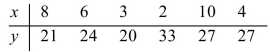
Compute the correlation coefficient. 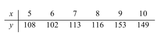
A) 0.117
B) 46.143
C) 0.779
D) 0.883
A) 0.117
B) 46.143
C) 0.779
D) 0.883
Question
Compute the least-squares regression line for predicting y from x given the following summary statistics: 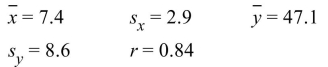
A) y=28.6666+2.4910 x
B) y=2.4910+28.6666 x
C) y=28.6666+0.2833 x
D) y=0.2833+28.6666 x
A) y=28.6666+2.4910 x
B) y=2.4910+28.6666 x
C) y=28.6666+0.2833 x
D) y=0.2833+28.6666 x
Question
One of the primary feeds for beef cattle is corn. The following table presents the average price in dollars for a bushel of corn and a pound of ribeye steak for 10 consecutive months. 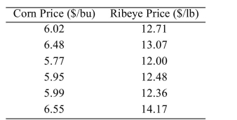 The least-squares regression line for predicting the ribeye price from the corn price is
 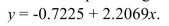 Predict the ribeye price in a month when the corn price was $6.28 per bushel.
A) $13.14 per lb
B) $14.52 per lb
C) $12.48 per lb
D) $13.86 per lb
The least-squares regression line for predicting the ribeye price from the corn price is Predict the ribeye price in a month when the corn price was $6.28 per bushel.A) $13.14 per lb
B) $14.52 per lb
C) $12.48 per lb
D) $13.86 per lb
Question
The following table lists the heights in inches and weights in pounds of six football quarterbacks. 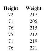 The least-squares regression equation is
 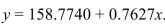 . If two quarterbacks differ in height by 6 inches, by how much would you predict their weights to differ?
A) 4.58 pounds
B) 0.76 pounds
C) 6.00 pounds
D) 952.64 pounds
The least-squares regression equation is . If two quarterbacks differ in height by 6 inches, by how much would you predict their weights to differ?A) 4.58 pounds
B) 0.76 pounds
C) 6.00 pounds
D) 952.64 pounds
Question
One of the primary feeds for beef cattle is corn. The following table presents the average price in dollars for a bushel of corn and a pound of ribeye steak for 10 consecutive months. 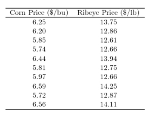 The correlation coefficient between the corn price and the ribeye price is 0.918. Which of the
Following is the best interpretation of the correlation coefficient?
A) The price of ribeye tends to go down and the price of corn goes up.
B) The changes in corn price and ribeye price tend to go up and down together.
C) There is no correlation between the price of corn and the price of ribeye.
D) Increasing corn prices cause ribeye prices to increase.
The correlation coefficient between the corn price and the ribeye price is 0.918. Which of theFollowing is the best interpretation of the correlation coefficient?
A) The price of ribeye tends to go down and the price of corn goes up.
B) The changes in corn price and ribeye price tend to go up and down together.
C) There is no correlation between the price of corn and the price of ribeye.
D) Increasing corn prices cause ribeye prices to increase.
Question
One of the primary feeds for beef cattle is corn. The following table presents the average price in dollars for a bushel of corn and a pound of ribeye steak for 10 consecutive months. 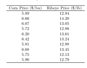 Construct a scatter plot of the price of ribeye (y) versus the price of corn (x).
A)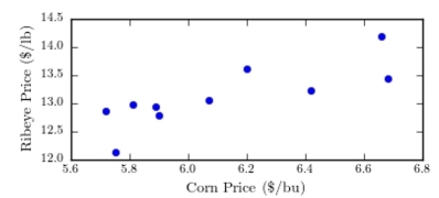
B)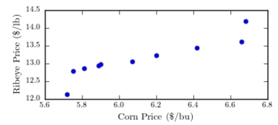
C)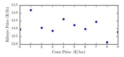
D)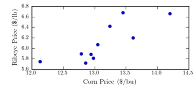
Construct a scatter plot of the price of ribeye (y) versus the price of corn (x). A)
B)
C)
D)
Question
For which of the following scatter plots is the correlation coefficient an appropriate summary?
A)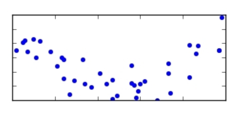
B)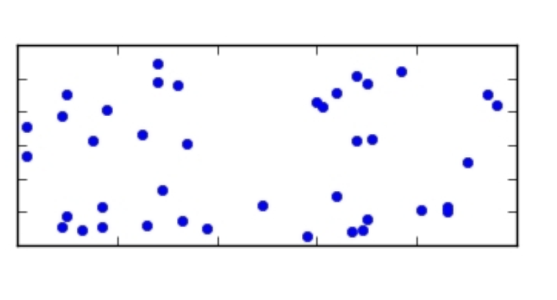
C)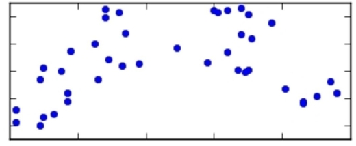
D)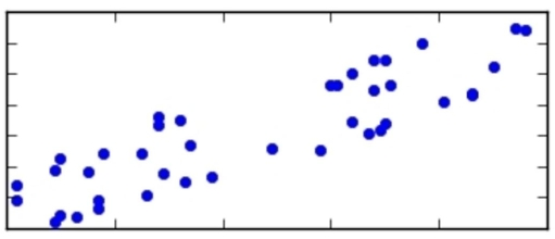
A)
B)
C)
D)
Question
The common cricket can be used as a crude thermometer. The colder the temperature, the slower the rate of chirping. The table below shows the average chirp rate of a cricket at various temperatures. 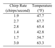 The least-squares regression line for predicting the temperature from the chirp rate is
 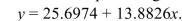 Predict the temperature if the chirp rate is 1.6 chirps per second.
A) 51 ºF
B) 48 ºF
C) 44 ºF
D) 22 ºF
The least-squares regression line for predicting the temperature from the chirp rate is Predict the temperature if the chirp rate is 1.6 chirps per second.A) 51 ºF
B) 48 ºF
C) 44 ºF
D) 22 ºF
Question
The following table presents the average price in dollars for a dozen eggs and a gallon of milk in several recent years. 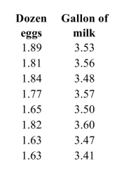 The least-squares regression equation is
 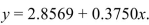 . If the price of eggs differs by $0.25
From one year to the next, by how much would you expect the price of milk to differ?
A) $1.50
B) -$0.09
C) $0.38
D) $0.09
The least-squares regression equation is . If the price of eggs differs by $0.25From one year to the next, by how much would you expect the price of milk to differ?
A) $1.50
B) -$0.09
C) $0.38
D) $0.09
Question
One of the primary feeds for beef cattle is corn. The following table presents the average price in dollars for a bushel of corn and a pound of ribeye steak for 10 consecutive months. 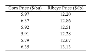 The least-squares regression line for predicting the ribeye price from the corn price is y = 6.3662 + 1.0315x.
If the price of corn differs by $0.15 per bushel, by how much would you expect the price of ribeye to
Differ?
A) $6.52 per lb
B) -$0.95 per lb
C) $0.15 per lb
D) $0.95 per lb
The least-squares regression line for predicting the ribeye price from the corn price is y = 6.3662 + 1.0315x.If the price of corn differs by $0.15 per bushel, by how much would you expect the price of ribeye to
Differ?
A) $6.52 per lb
B) -$0.95 per lb
C) $0.15 per lb
D) $0.95 per lb
Question
The common cricket can be used as a crude thermometer. The colder the temperature, the slower the rate of chirping. The table below shows the average chirp rate of a cricket at various temperatures. 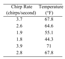 Compute the least-squares regression line for predicting the temperature from the chirp rate.
A) y=9.9492+34.0748 x
B) y=12.7143+34.0748 x
C) y=34.0748+12.7143 x
D) y=34.0748+9.9492 x
Compute the least-squares regression line for predicting the temperature from the chirp rate. A) y=9.9492+34.0748 x
B) y=12.7143+34.0748 x
C) y=34.0748+12.7143 x
D) y=34.0748+9.9492 x
Question
The following table presents the number of police officers (per 100,000 citizens) and the annual murder rate (per 100,000 citizens) for a sample of cities. 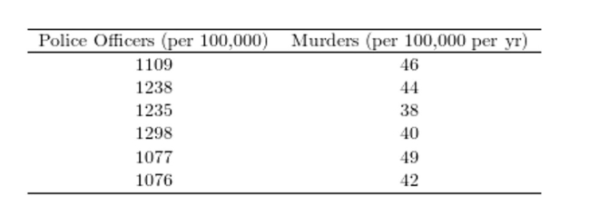 Compute the correlation coefficient between the per capita number of police officers and the per capita
Murder rate.
A) -0.726
B) -0.666
C) 0.444
D) -0.444
Compute the correlation coefficient between the per capita number of police officers and the per capitaMurder rate.
A) -0.726
B) -0.666
C) 0.444
D) -0.444
Question
The common cricket can be used as a crude thermometer. The colder the temperature, the slower the rate of chirping. The table below shows the average chirp rate of a cricket at various temperatures. 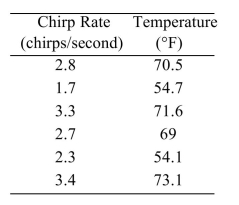 The least-squares regression line for predicting the temperature from the chirp rate is y = 32.298 + 12.297x.
If two chirp rates differ by 1.5 chirps per second, by how much would the temperature differ?
A) 48 ºF
B) 17 ºF
C) 18 ºF
D) 21 ºF
The least-squares regression line for predicting the temperature from the chirp rate is y = 32.298 + 12.297x.If two chirp rates differ by 1.5 chirps per second, by how much would the temperature differ?
A) 48 ºF
B) 17 ºF
C) 18 ºF
D) 21 ºF
Question
The following table presents the number of police officers (per 100,000 citizens) and the annual murder rate (per 100,000 citizens) for a sample of cities. 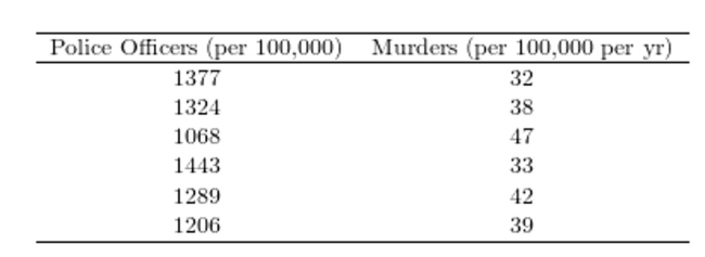 Construct a scatter plot of the per capita murder rate (y) versus the per capita number of police officers(x))
A)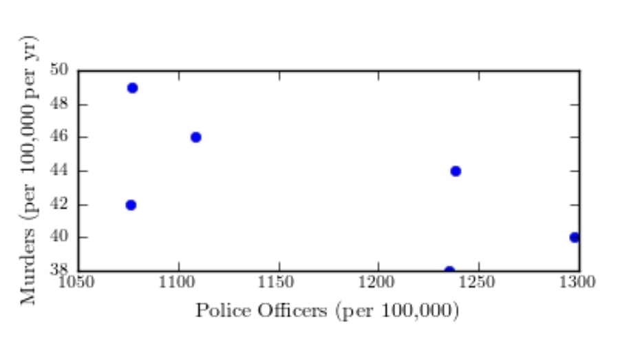
B)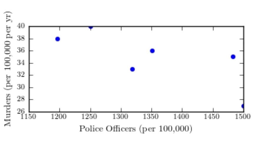
C)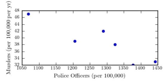
D)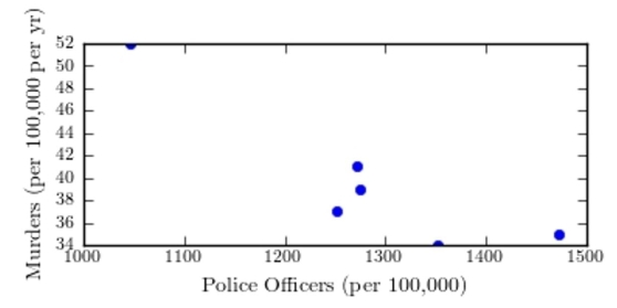
Construct a scatter plot of the per capita murder rate (y) versus the per capita number of police officers(x)) A)
B)
C)
D)
Question
One of the primary feeds for beef cattle is corn. The following table presents the average price in dollars for a bushel of corn and a pound of ribeye steak for 10 consecutive months. 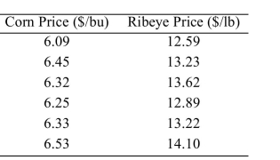 Compute the least-squares regression line for predicting the ribeye price from the corn price.
A) y=-5.491+0.3372 x
B) y=2.9654-5.491 x
C) y=5.491+0.3372 x
D) y=-5.491+2.9654 x
Compute the least-squares regression line for predicting the ribeye price from the corn price. A) y=-5.491+0.3372 x
B) y=2.9654-5.491 x
C) y=5.491+0.3372 x
D) y=-5.491+2.9654 x
Question
A blood pressure measurement consists of two numbers: the systolic pressure, which is the maximum pressure taken when the heart is contracting, and the diastolic pressure, which is the
Minimum pressure taken at the beginning of the heartbeat. Blood pressures were measured, in
Millimeters of mercury (mmHg), for a sample of eight adults. The following table presents the
Results.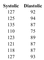 The least-squares regression equation is
 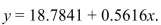 . If the systolic pressures of two patients
Differ by 8 mmHg, by how much would you predict their diastolic pressures to differ?
A) 8.56 mmHg
B) 4.49 mmHg
C) 0.56 mmHg
D) 0.07 mmHg
Minimum pressure taken at the beginning of the heartbeat. Blood pressures were measured, in
Millimeters of mercury (mmHg), for a sample of eight adults. The following table presents the
Results.
The least-squares regression equation is . If the systolic pressures of two patientsDiffer by 8 mmHg, by how much would you predict their diastolic pressures to differ?
A) 8.56 mmHg
B) 4.49 mmHg
C) 0.56 mmHg
D) 0.07 mmHg
Question
The following table presents the number of police officers (per 100,000 citizens) and the annual murder rate (per 100,000 citizens) for a sample of cities. 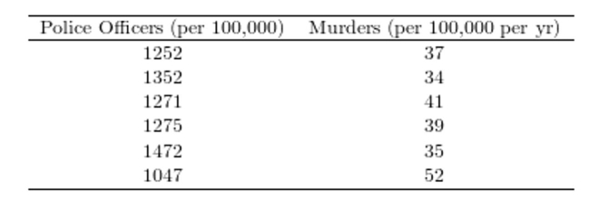 The correlation coefficient between the per capita number of police officers and the per capita murder rates
-0)899. Which of the following is the best interpretation of the correlation coefficient?
A) The per capita murder rate tends to go down as the per capita number of police officers goes up.
B) Higher murder rates make it more difficult for cities to hire police officers.
C) The per capita number of police officers and the per capita murder rates are positively associated.
D) More per capita police officers results in fewer per capita murders.
The correlation coefficient between the per capita number of police officers and the per capita murder rates-0)899. Which of the following is the best interpretation of the correlation coefficient?
A) The per capita murder rate tends to go down as the per capita number of police officers goes up.
B) Higher murder rates make it more difficult for cities to hire police officers.
C) The per capita number of police officers and the per capita murder rates are positively associated.
D) More per capita police officers results in fewer per capita murders.
Question
Characterize the relationship shown in the figure. 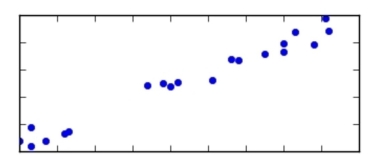
A) positive linear
B) positive nonlinear
C) negative nonlinear
D) negative linear
A) positive linear
B) positive nonlinear
C) negative nonlinear
D) negative linear
Question
The following table shows the per-person carbon dioxide emissions for the United States and for the rest of the world over six years. 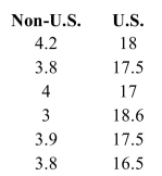 The least-squares regression equation is
 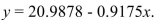 . If the non-U.S. emissions differ by 0.5
From one year to the next, by how much would you predict the U.S. emissions to differ?
A) -0.92
B) 0.46
C) -1.83
D) -0.46
The least-squares regression equation is . If the non-U.S. emissions differ by 0.5From one year to the next, by how much would you predict the U.S. emissions to differ?
A) -0.92
B) 0.46
C) -1.83
D) -0.46
Question
One of the primary feeds for beef cattle is corn. The following table presents the average price in dollars for a bushel of corn and a pound of ribeye steak for 10 consecutive months. 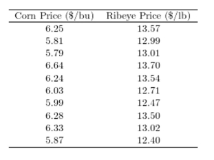 Compute the correlation coefficient between the corn price and the ribeye price.
A) 0.621
B) 0.721
C) 0.279
D) 0.520
Compute the correlation coefficient between the corn price and the ribeye price.A) 0.621
B) 0.721
C) 0.279
D) 0.520
Question
The following MINITAB output presents the least squares regression line for predicting the price of a certain commodity from the price of a barrel of oil. 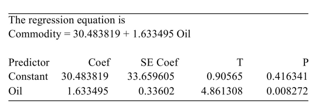 Write the equation of the least-squares regression line.
A) y=30.483819+1.633495 x
B) y=0.90565+4.861308 x
C) y=0.416341+0.008272 x
D) y=1.633495+30.483819 x
Write the equation of the least-squares regression line. A) y=30.483819+1.633495 x
B) y=0.90565+4.861308 x
C) y=0.416341+0.008272 x
D) y=1.633495+30.483819 x
Question
An automotive engineer computed a least-squares regression line for predicting the gas mileage (miles per gallon, or mpg) of a certain vehicle from its speed in mph. The results are presented in
The following Excel output.
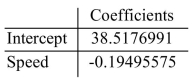
Predict the gas mileage when the vehicle is traveling at 56 mph.
A) 25.2 mpg
B) 49 mpg
C) 28 mpg
D) 31 mpg
The following Excel output.
Predict the gas mileage when the vehicle is traveling at 56 mph.
A) 25.2 mpg
B) 49 mpg
C) 28 mpg
D) 31 mpg
Question
The following display from a graphing calculator presents the least-squares regression line for predicting the price of a certain commodity (y) from the price of a barrel of oil (x). 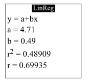 Write the equation of the least-squares regression line.
A) y=4.71+0.48909 x
B) y=4.71+0.49 x
C) y=0.49+0.48909 x
D) y=0.49+4.71 x
Write the equation of the least-squares regression line. A) y=4.71+0.48909 x
B) y=4.71+0.49 x
C) y=0.49+0.48909 x
D) y=0.49+4.71 x
Question
The following display from a graphing calculator presents the least-squares regression line for predicting the price of a certain commodity (y) from the price of a barrel of oil (x). 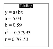 What is the correlation between the oil price and the commodity price?
A) 0.76153
B) 0.59
C) 5.04
D) 0.57993
What is the correlation between the oil price and the commodity price?A) 0.76153
B) 0.59
C) 5.04
D) 0.57993
Question
An automotive engineer computed a least-squares regression line for predicting the gas mileage (mile per gallon) of a certain vehicle from its speed in mph. The results are presented in the
Following Excel output.
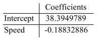
Write the equation of the least-squares regression line.
A) y=-38.394979+0.18832886 x
B) y=38.3949789-0.18832886 x
C) y=38.3949789+0.18832886 x
D) y=-0.18832886+38.3949789 x
Following Excel output.
Write the equation of the least-squares regression line.
A) y=-38.394979+0.18832886 x
B) y=38.3949789-0.18832886 x
C) y=38.3949789+0.18832886 x
D) y=-0.18832886+38.3949789 x
Question
As with many other construction materials, the price of gravel (per ton) depends on the quantity of material ordered. The following table presents the unit cost (dollars/ton) for gravel for various order sizes (in
Tons).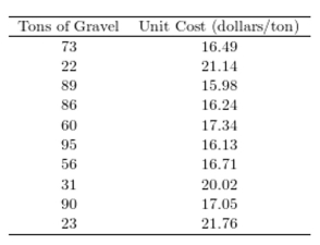 Compute the coefficient of determination.
A) -0.0767
B) -0.9233
C) 0.8525
D) 0.1475
Tons).
Compute the coefficient of determination.A) -0.0767
B) -0.9233
C) 0.8525
D) 0.1475
Question
For the following data set, how much of the variation in the outcome variable is explained by the least-squares regression line? 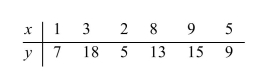
A) 48.1%
B) 73.1%
C) 26.9%
D) 51.9%
A) 48.1%
B) 73.1%
C) 26.9%
D) 51.9%
Question
For the following data set, compute the coefficient of determination.
A) 0.272
B) 0.728
C) 0.074
D) 0.926
A) 0.272
B) 0.728
C) 0.074
D) 0.926
Question
The following MINITAB output presents the lest squares regression line for predicting the price of a certain commodity from the price of a barrel of oil. 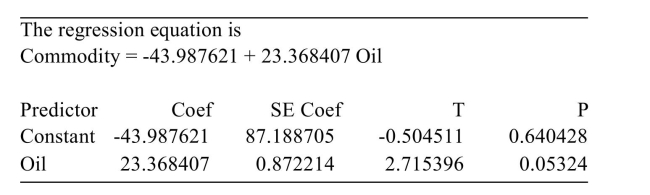 Predict the commodity price when the oil price is $114 per barrel.
A) $215
B) $226
C) $249
D) $170
Predict the commodity price when the oil price is $114 per barrel.A) $215
B) $226
C) $249
D) $170
Question
Of points 1, 2, and 3 shown below, which is the most influential? 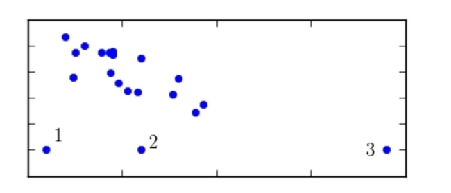
A) point 1
B) point 3
C) All have the same influence.
D) point 2
A) point 1
B) point 3
C) All have the same influence.
D) point 2
Question
MINITAB-style residual plots are shown below. Which one of these plots indicates that it was appropriate to compute a least-squares regression line?
A)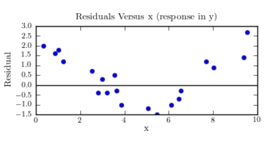
B)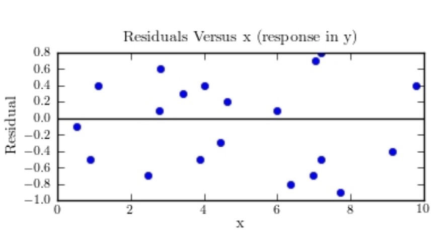
C)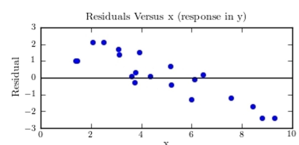
D)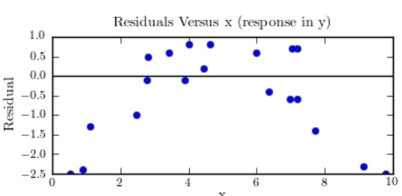
A)
B)
C)
D)
Question
As with many other construction materials, the price of gravel (per ton) depends on the quantity of material ordered. The following table presents the unit cost (dollars/ton) for gravel for various order sizes (in tons). 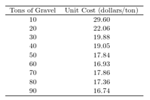 Which of the following graphs is the correct residual plot for the data set? (Hint: create your own residual plot
And compare it to those shown below.)
A)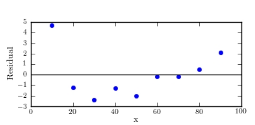
B)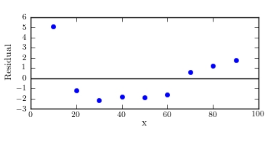
C)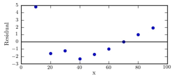
D)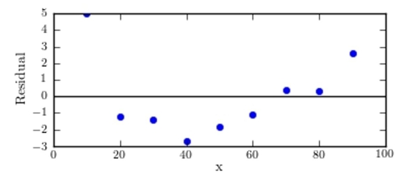
Which of the following graphs is the correct residual plot for the data set? (Hint: create your own residual plotAnd compare it to those shown below.)
A)
B)
C)
D)
Question
The following display from a graphing calculator presents the least-squares regression line for predicting the price of a certain commodity (y) from the price of a barrel of oil (x). 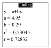 Predict the commodity price when oil costs $107 per barrel.
A) $62
B) $530
C) $83
D) $36
Predict the commodity price when oil costs $107 per barrel.A) $62
B) $530
C) $83
D) $36

Unlock Deck
Sign up to unlock the cards in this deck!
Unlock Deck
Unlock Deck
1/33
Play
Full screen (f)
Deck 4: Summarizing Bivariate Data
1
Compute the correlation coefficient.
A) 0.117
B) 46.143
C) 0.779
D) 0.883
A) 0.117
B) 46.143
C) 0.779
D) 0.883
0.883
2
Compute the least-squares regression line for predicting y from x given the following summary statistics:
A) y=28.6666+2.4910 x
B) y=2.4910+28.6666 x
C) y=28.6666+0.2833 x
D) y=0.2833+28.6666 x
A) y=28.6666+2.4910 x
B) y=2.4910+28.6666 x
C) y=28.6666+0.2833 x
D) y=0.2833+28.6666 x
y=28.6666+2.4910 x
3
One of the primary feeds for beef cattle is corn. The following table presents the average price in dollars for a bushel of corn and a pound of ribeye steak for 10 consecutive months. The least-squares regression line for predicting the ribeye price from the corn price is Predict the ribeye price in a month when the corn price was $6.28 per bushel.
A) $13.14 per lb
B) $14.52 per lb
C) $12.48 per lb
D) $13.86 per lb
The least-squares regression line for predicting the ribeye price from the corn price is Predict the ribeye price in a month when the corn price was $6.28 per bushel.A) $13.14 per lb
B) $14.52 per lb
C) $12.48 per lb
D) $13.86 per lb
$13.14 per lb
4
The following table lists the heights in inches and weights in pounds of six football quarterbacks. The least-squares regression equation is . If two quarterbacks differ in height by 6 inches, by how much would you predict their weights to differ?
A) 4.58 pounds
B) 0.76 pounds
C) 6.00 pounds
D) 952.64 pounds
The least-squares regression equation is . If two quarterbacks differ in height by 6 inches, by how much would you predict their weights to differ?A) 4.58 pounds
B) 0.76 pounds
C) 6.00 pounds
D) 952.64 pounds
Unlock Deck
Unlock for access to all 33 flashcards in this deck.
Unlock Deck
k this deck
5
One of the primary feeds for beef cattle is corn. The following table presents the average price in dollars for a bushel of corn and a pound of ribeye steak for 10 consecutive months. The correlation coefficient between the corn price and the ribeye price is 0.918. Which of the
Following is the best interpretation of the correlation coefficient?
A) The price of ribeye tends to go down and the price of corn goes up.
B) The changes in corn price and ribeye price tend to go up and down together.
C) There is no correlation between the price of corn and the price of ribeye.
D) Increasing corn prices cause ribeye prices to increase.
The correlation coefficient between the corn price and the ribeye price is 0.918. Which of theFollowing is the best interpretation of the correlation coefficient?
A) The price of ribeye tends to go down and the price of corn goes up.
B) The changes in corn price and ribeye price tend to go up and down together.
C) There is no correlation between the price of corn and the price of ribeye.
D) Increasing corn prices cause ribeye prices to increase.
Unlock Deck
Unlock for access to all 33 flashcards in this deck.
Unlock Deck
k this deck
6
One of the primary feeds for beef cattle is corn. The following table presents the average price in dollars for a bushel of corn and a pound of ribeye steak for 10 consecutive months. Construct a scatter plot of the price of ribeye (y) versus the price of corn (x).
A)
B)
C)
D)
Construct a scatter plot of the price of ribeye (y) versus the price of corn (x). A)
B)
C)
D)
Unlock Deck
Unlock for access to all 33 flashcards in this deck.
Unlock Deck
k this deck
7
For which of the following scatter plots is the correlation coefficient an appropriate summary?
A)
B)
C)
D)
A)
B)
C)
D)
Unlock Deck
Unlock for access to all 33 flashcards in this deck.
Unlock Deck
k this deck
8
The common cricket can be used as a crude thermometer. The colder the temperature, the slower the rate of chirping. The table below shows the average chirp rate of a cricket at various temperatures. The least-squares regression line for predicting the temperature from the chirp rate is Predict the temperature if the chirp rate is 1.6 chirps per second.
A) 51 ºF
B) 48 ºF
C) 44 ºF
D) 22 ºF
The least-squares regression line for predicting the temperature from the chirp rate is Predict the temperature if the chirp rate is 1.6 chirps per second.A) 51 ºF
B) 48 ºF
C) 44 ºF
D) 22 ºF
Unlock Deck
Unlock for access to all 33 flashcards in this deck.
Unlock Deck
k this deck
9
The following table presents the average price in dollars for a dozen eggs and a gallon of milk in several recent years. The least-squares regression equation is . If the price of eggs differs by $0.25
From one year to the next, by how much would you expect the price of milk to differ?
A) $1.50
B) -$0.09
C) $0.38
D) $0.09
The least-squares regression equation is . If the price of eggs differs by $0.25From one year to the next, by how much would you expect the price of milk to differ?
A) $1.50
B) -$0.09
C) $0.38
D) $0.09
Unlock Deck
Unlock for access to all 33 flashcards in this deck.
Unlock Deck
k this deck
10
One of the primary feeds for beef cattle is corn. The following table presents the average price in dollars for a bushel of corn and a pound of ribeye steak for 10 consecutive months. The least-squares regression line for predicting the ribeye price from the corn price is y = 6.3662 + 1.0315x.
If the price of corn differs by $0.15 per bushel, by how much would you expect the price of ribeye to
Differ?
A) $6.52 per lb
B) -$0.95 per lb
C) $0.15 per lb
D) $0.95 per lb
The least-squares regression line for predicting the ribeye price from the corn price is y = 6.3662 + 1.0315x.If the price of corn differs by $0.15 per bushel, by how much would you expect the price of ribeye to
Differ?
A) $6.52 per lb
B) -$0.95 per lb
C) $0.15 per lb
D) $0.95 per lb
Unlock Deck
Unlock for access to all 33 flashcards in this deck.
Unlock Deck
k this deck
11
The common cricket can be used as a crude thermometer. The colder the temperature, the slower the rate of chirping. The table below shows the average chirp rate of a cricket at various temperatures. Compute the least-squares regression line for predicting the temperature from the chirp rate.
A) y=9.9492+34.0748 x
B) y=12.7143+34.0748 x
C) y=34.0748+12.7143 x
D) y=34.0748+9.9492 x
Compute the least-squares regression line for predicting the temperature from the chirp rate. A) y=9.9492+34.0748 x
B) y=12.7143+34.0748 x
C) y=34.0748+12.7143 x
D) y=34.0748+9.9492 x
Unlock Deck
Unlock for access to all 33 flashcards in this deck.
Unlock Deck
k this deck
12
The following table presents the number of police officers (per 100,000 citizens) and the annual murder rate (per 100,000 citizens) for a sample of cities. Compute the correlation coefficient between the per capita number of police officers and the per capita
Murder rate.
A) -0.726
B) -0.666
C) 0.444
D) -0.444
Compute the correlation coefficient between the per capita number of police officers and the per capitaMurder rate.
A) -0.726
B) -0.666
C) 0.444
D) -0.444
Unlock Deck
Unlock for access to all 33 flashcards in this deck.
Unlock Deck
k this deck
13
The common cricket can be used as a crude thermometer. The colder the temperature, the slower the rate of chirping. The table below shows the average chirp rate of a cricket at various temperatures. The least-squares regression line for predicting the temperature from the chirp rate is y = 32.298 + 12.297x.
If two chirp rates differ by 1.5 chirps per second, by how much would the temperature differ?
A) 48 ºF
B) 17 ºF
C) 18 ºF
D) 21 ºF
The least-squares regression line for predicting the temperature from the chirp rate is y = 32.298 + 12.297x.If two chirp rates differ by 1.5 chirps per second, by how much would the temperature differ?
A) 48 ºF
B) 17 ºF
C) 18 ºF
D) 21 ºF
Unlock Deck
Unlock for access to all 33 flashcards in this deck.
Unlock Deck
k this deck
14
The following table presents the number of police officers (per 100,000 citizens) and the annual murder rate (per 100,000 citizens) for a sample of cities. Construct a scatter plot of the per capita murder rate (y) versus the per capita number of police officers(x))
A)
B)
C)
D)
Construct a scatter plot of the per capita murder rate (y) versus the per capita number of police officers(x)) A)
B)
C)
D)
Unlock Deck
Unlock for access to all 33 flashcards in this deck.
Unlock Deck
k this deck
15
One of the primary feeds for beef cattle is corn. The following table presents the average price in dollars for a bushel of corn and a pound of ribeye steak for 10 consecutive months. Compute the least-squares regression line for predicting the ribeye price from the corn price.
A) y=-5.491+0.3372 x
B) y=2.9654-5.491 x
C) y=5.491+0.3372 x
D) y=-5.491+2.9654 x
Compute the least-squares regression line for predicting the ribeye price from the corn price. A) y=-5.491+0.3372 x
B) y=2.9654-5.491 x
C) y=5.491+0.3372 x
D) y=-5.491+2.9654 x
Unlock Deck
Unlock for access to all 33 flashcards in this deck.
Unlock Deck
k this deck
16
A blood pressure measurement consists of two numbers: the systolic pressure, which is the maximum pressure taken when the heart is contracting, and the diastolic pressure, which is the
Minimum pressure taken at the beginning of the heartbeat. Blood pressures were measured, in
Millimeters of mercury (mmHg), for a sample of eight adults. The following table presents the
Results. The least-squares regression equation is . If the systolic pressures of two patients
Differ by 8 mmHg, by how much would you predict their diastolic pressures to differ?
A) 8.56 mmHg
B) 4.49 mmHg
C) 0.56 mmHg
D) 0.07 mmHg
Minimum pressure taken at the beginning of the heartbeat. Blood pressures were measured, in
Millimeters of mercury (mmHg), for a sample of eight adults. The following table presents the
Results.
The least-squares regression equation is . If the systolic pressures of two patientsDiffer by 8 mmHg, by how much would you predict their diastolic pressures to differ?
A) 8.56 mmHg
B) 4.49 mmHg
C) 0.56 mmHg
D) 0.07 mmHg
Unlock Deck
Unlock for access to all 33 flashcards in this deck.
Unlock Deck
k this deck
17
The following table presents the number of police officers (per 100,000 citizens) and the annual murder rate (per 100,000 citizens) for a sample of cities. The correlation coefficient between the per capita number of police officers and the per capita murder rates
-0)899. Which of the following is the best interpretation of the correlation coefficient?
A) The per capita murder rate tends to go down as the per capita number of police officers goes up.
B) Higher murder rates make it more difficult for cities to hire police officers.
C) The per capita number of police officers and the per capita murder rates are positively associated.
D) More per capita police officers results in fewer per capita murders.
The correlation coefficient between the per capita number of police officers and the per capita murder rates-0)899. Which of the following is the best interpretation of the correlation coefficient?
A) The per capita murder rate tends to go down as the per capita number of police officers goes up.
B) Higher murder rates make it more difficult for cities to hire police officers.
C) The per capita number of police officers and the per capita murder rates are positively associated.
D) More per capita police officers results in fewer per capita murders.
Unlock Deck
Unlock for access to all 33 flashcards in this deck.
Unlock Deck
k this deck
18
Characterize the relationship shown in the figure.
A) positive linear
B) positive nonlinear
C) negative nonlinear
D) negative linear
A) positive linear
B) positive nonlinear
C) negative nonlinear
D) negative linear
Unlock Deck
Unlock for access to all 33 flashcards in this deck.
Unlock Deck
k this deck
19
The following table shows the per-person carbon dioxide emissions for the United States and for the rest of the world over six years. The least-squares regression equation is . If the non-U.S. emissions differ by 0.5
From one year to the next, by how much would you predict the U.S. emissions to differ?
A) -0.92
B) 0.46
C) -1.83
D) -0.46
The least-squares regression equation is . If the non-U.S. emissions differ by 0.5From one year to the next, by how much would you predict the U.S. emissions to differ?
A) -0.92
B) 0.46
C) -1.83
D) -0.46
Unlock Deck
Unlock for access to all 33 flashcards in this deck.
Unlock Deck
k this deck
20
One of the primary feeds for beef cattle is corn. The following table presents the average price in dollars for a bushel of corn and a pound of ribeye steak for 10 consecutive months. Compute the correlation coefficient between the corn price and the ribeye price.
A) 0.621
B) 0.721
C) 0.279
D) 0.520
Compute the correlation coefficient between the corn price and the ribeye price.A) 0.621
B) 0.721
C) 0.279
D) 0.520
Unlock Deck
Unlock for access to all 33 flashcards in this deck.
Unlock Deck
k this deck
21
The following MINITAB output presents the least squares regression line for predicting the price of a certain commodity from the price of a barrel of oil. Write the equation of the least-squares regression line.
A) y=30.483819+1.633495 x
B) y=0.90565+4.861308 x
C) y=0.416341+0.008272 x
D) y=1.633495+30.483819 x
Write the equation of the least-squares regression line. A) y=30.483819+1.633495 x
B) y=0.90565+4.861308 x
C) y=0.416341+0.008272 x
D) y=1.633495+30.483819 x
Unlock Deck
Unlock for access to all 33 flashcards in this deck.
Unlock Deck
k this deck
22
An automotive engineer computed a least-squares regression line for predicting the gas mileage (miles per gallon, or mpg) of a certain vehicle from its speed in mph. The results are presented in
The following Excel output.
Predict the gas mileage when the vehicle is traveling at 56 mph.
A) 25.2 mpg
B) 49 mpg
C) 28 mpg
D) 31 mpg
The following Excel output.
Predict the gas mileage when the vehicle is traveling at 56 mph.
A) 25.2 mpg
B) 49 mpg
C) 28 mpg
D) 31 mpg
Unlock Deck
Unlock for access to all 33 flashcards in this deck.
Unlock Deck
k this deck
23
The following display from a graphing calculator presents the least-squares regression line for predicting the price of a certain commodity (y) from the price of a barrel of oil (x). Write the equation of the least-squares regression line.
A) y=4.71+0.48909 x
B) y=4.71+0.49 x
C) y=0.49+0.48909 x
D) y=0.49+4.71 x
Write the equation of the least-squares regression line. A) y=4.71+0.48909 x
B) y=4.71+0.49 x
C) y=0.49+0.48909 x
D) y=0.49+4.71 x
Unlock Deck
Unlock for access to all 33 flashcards in this deck.
Unlock Deck
k this deck
24
The following display from a graphing calculator presents the least-squares regression line for predicting the price of a certain commodity (y) from the price of a barrel of oil (x). What is the correlation between the oil price and the commodity price?
A) 0.76153
B) 0.59
C) 5.04
D) 0.57993
What is the correlation between the oil price and the commodity price?A) 0.76153
B) 0.59
C) 5.04
D) 0.57993
Unlock Deck
Unlock for access to all 33 flashcards in this deck.
Unlock Deck
k this deck
25
An automotive engineer computed a least-squares regression line for predicting the gas mileage (mile per gallon) of a certain vehicle from its speed in mph. The results are presented in the
Following Excel output.
Write the equation of the least-squares regression line.
A) y=-38.394979+0.18832886 x
B) y=38.3949789-0.18832886 x
C) y=38.3949789+0.18832886 x
D) y=-0.18832886+38.3949789 x
Following Excel output.
Write the equation of the least-squares regression line.
A) y=-38.394979+0.18832886 x
B) y=38.3949789-0.18832886 x
C) y=38.3949789+0.18832886 x
D) y=-0.18832886+38.3949789 x
Unlock Deck
Unlock for access to all 33 flashcards in this deck.
Unlock Deck
k this deck
26
As with many other construction materials, the price of gravel (per ton) depends on the quantity of material ordered. The following table presents the unit cost (dollars/ton) for gravel for various order sizes (in
Tons). Compute the coefficient of determination.
A) -0.0767
B) -0.9233
C) 0.8525
D) 0.1475
Tons).
Compute the coefficient of determination.A) -0.0767
B) -0.9233
C) 0.8525
D) 0.1475
Unlock Deck
Unlock for access to all 33 flashcards in this deck.
Unlock Deck
k this deck
27
For the following data set, how much of the variation in the outcome variable is explained by the least-squares regression line?
A) 48.1%
B) 73.1%
C) 26.9%
D) 51.9%
A) 48.1%
B) 73.1%
C) 26.9%
D) 51.9%
Unlock Deck
Unlock for access to all 33 flashcards in this deck.
Unlock Deck
k this deck
28
For the following data set, compute the coefficient of determination.
A) 0.272
B) 0.728
C) 0.074
D) 0.926
A) 0.272
B) 0.728
C) 0.074
D) 0.926
Unlock Deck
Unlock for access to all 33 flashcards in this deck.
Unlock Deck
k this deck
29
The following MINITAB output presents the lest squares regression line for predicting the price of a certain commodity from the price of a barrel of oil. Predict the commodity price when the oil price is $114 per barrel.
A) $215
B) $226
C) $249
D) $170
Predict the commodity price when the oil price is $114 per barrel.A) $215
B) $226
C) $249
D) $170
Unlock Deck
Unlock for access to all 33 flashcards in this deck.
Unlock Deck
k this deck
30
Of points 1, 2, and 3 shown below, which is the most influential?
A) point 1
B) point 3
C) All have the same influence.
D) point 2
A) point 1
B) point 3
C) All have the same influence.
D) point 2
Unlock Deck
Unlock for access to all 33 flashcards in this deck.
Unlock Deck
k this deck
31
MINITAB-style residual plots are shown below. Which one of these plots indicates that it was appropriate to compute a least-squares regression line?
A)
B)
C)
D)
A)
B)
C)
D)
Unlock Deck
Unlock for access to all 33 flashcards in this deck.
Unlock Deck
k this deck
32
As with many other construction materials, the price of gravel (per ton) depends on the quantity of material ordered. The following table presents the unit cost (dollars/ton) for gravel for various order sizes (in tons). Which of the following graphs is the correct residual plot for the data set? (Hint: create your own residual plot
And compare it to those shown below.)
A)
B)
C)
D)
Which of the following graphs is the correct residual plot for the data set? (Hint: create your own residual plotAnd compare it to those shown below.)
A)
B)
C)
D)
Unlock Deck
Unlock for access to all 33 flashcards in this deck.
Unlock Deck
k this deck
33
The following display from a graphing calculator presents the least-squares regression line for predicting the price of a certain commodity (y) from the price of a barrel of oil (x). Predict the commodity price when oil costs $107 per barrel.
A) $62
B) $530
C) $83
D) $36
Predict the commodity price when oil costs $107 per barrel.A) $62
B) $530
C) $83
D) $36
Unlock Deck
Unlock for access to all 33 flashcards in this deck.
Unlock Deck
k this deck
Unlock Deck
Unlock for access to all 33 flashcards in this deck.


