Deck 7: Production Economics
Full screen (f)
Question
Consider Exercise again. Suppose the owner of the trawler can sell all the fishcaught for $75 per 100 pounds and can hire as many crew members as desired by paying them $150 per week. Assuming that the owner of the trawler is interested in maximizing profits, determine the optimal crew size.
Exercise
The amount of fish caught per week on a trawler is a function of the crew size assigned to operate the boat. Based on past data, the following production schedule was developed:
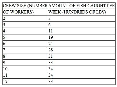 a. Over what ranges of workers are there (i) increasing, (ii) constant, (iii) decreasing, and (iv) negative returns
b. How large a crew should be used if the trawler owner is interested in maximizing the total amount of fish caught
c. How large a crew should be used if the trawler owner is interested in maximizing the average amount of fish caught per person
Exercise
The amount of fish caught per week on a trawler is a function of the crew size assigned to operate the boat. Based on past data, the following production schedule was developed:
a. Over what ranges of workers are there (i) increasing, (ii) constant, (iii) decreasing, and (iv) negative returns b. How large a crew should be used if the trawler owner is interested in maximizing the total amount of fish caught
c. How large a crew should be used if the trawler owner is interested in maximizing the average amount of fish caught per person
Question
Determine whether this production function exhibits increasing, decreasing, or constant returns to scale. (Ignore the issue of statistical significance.)
Question
Question
Question
Question
Based on the production function parameter estimates reported in Table:
a. Which industry (or industries) appears to exhibit decreasing returns to scale (Ignore the issue of statistical significance.)
b. Which industry comes closest to exhibiting constant returns to scale
c. In which industry will a given percentage increase in capital result in the largest percentage increase in output
d. In what industry will a given percentage increase in production workers result in the largest percentage increase in output
Table PRODUCTION ELASTICITIES FOR SEVERAL INDUSTRIES
 Number in parentheses below each elasticity coefficient is the standard error.
*Significantly greater than 1.0 at the 0.05 level (one-tailed test).
Source: John R. Moroney, "Cobb-Douglas Production Functions and Returns to Scale in U.S. Manufacturing Industry," Western Economic Journal 6, no. 1 (December 1967), Table 1, p. 46.
a. Which industry (or industries) appears to exhibit decreasing returns to scale (Ignore the issue of statistical significance.)
b. Which industry comes closest to exhibiting constant returns to scale
c. In which industry will a given percentage increase in capital result in the largest percentage increase in output
d. In what industry will a given percentage increase in production workers result in the largest percentage increase in output
Table PRODUCTION ELASTICITIES FOR SEVERAL INDUSTRIES
Number in parentheses below each elasticity coefficient is the standard error.*Significantly greater than 1.0 at the 0.05 level (one-tailed test).
Source: John R. Moroney, "Cobb-Douglas Production Functions and Returns to Scale in U.S. Manufacturing Industry," Western Economic Journal 6, no. 1 (December 1967), Table 1, p. 46.
Question
Consider the following Cobb-Douglas production function for the bus transportation system in a particular city:

where L = labor input in worker hours
F = fuel input in gallons
K = capital input in number of buses
Q = output measured in millions of bus miles
Suppose that the parameters ( , 1, 2, and 3) of this model were estimated using annual data for the past 25 years. The following results were obtained:
= 0.0012 1 = 0.45 2 = 0.20 3 = 0.30
a. Determine the (i) labor, (ii) fuel, and (iii) capital input production elasticities.
b. Suppose that labor input (worker hours) is increased by 2 percent next year (with the other inputs held constant). Determine the approximate percentage change in output.
c. Suppose that capital input (number of buses) is decreased by 3 percent next year (when certain older buses are taken out of service). Assuming that the other inputs are held constant, determine the approximate percentage changein output.
d. What type of returns to scale appears to characterize this bus transportation system (Ignore the issue of statistical significance.)
e. Discuss some of the methodological and measurement problems one might encounter in using time-series data to estimate the parameters of this model.
Question
Extension of the Cobb-Douglas Production Function-The Cobb-Douglas production function (Equation) can be shown to be a special case of a larger class of linear homogeneous production functions having the following mathematical form: 11
![Extension of the Cobb-Douglas Production Function-The Cobb-Douglas production function (Equation) can be shown to be a special case of a larger class of linear homogeneous production functions having the following mathematical form: 11 where is an efficiency parameter that shows the output resulting from given quantities of inputs; is a distribution parameter (0 1) that indicates the division of factor income between capital and labor; is a substitution parameter that is a measure of substitutability of capital for labor (or vice versa) in the production process; and is a scale parameter ( 0) that indicates the type of returns to scale (increasing, constant, or decreasing). Show that when = 1, this function exhibits constant returns to scale. [Hint: Increase capital K and labor L each by a factor of , or K* = ( )K and L* = ( )L, and show that output Q also increases by a factor of , or Q* = ( )(Q).] Equation 11 See R. G. Chambers, Applied Production Analysis (Cambridge: Cambridge University Press, 1988).<div style=padding-top: 35px>](https://d2lvgg3v3hfg70.cloudfront.net/SM2912/11eb7696_eeb0_85e4_adfc_9ba919dd5c96_SM2912_00.jpg)
where is an efficiency parameter that shows the output resulting from given quantities of inputs; is a distribution parameter (0 1) that indicates the division of factor income between capital and labor; is a substitution parameter that is a measure of substitutability of capital for labor (or vice versa) in the production process; and is a scale parameter ( 0) that indicates the type of returns to scale (increasing, constant, or decreasing). Show that when = 1, this function exhibits constant returns to scale. [Hint: Increase capital K and labor L each by a factor of , or K* = ( )K and L* = ( )L, and show that output Q also increases by a factor of , or Q* = ( )(Q).]
Equation
![Extension of the Cobb-Douglas Production Function-The Cobb-Douglas production function (Equation) can be shown to be a special case of a larger class of linear homogeneous production functions having the following mathematical form: 11 where is an efficiency parameter that shows the output resulting from given quantities of inputs; is a distribution parameter (0 1) that indicates the division of factor income between capital and labor; is a substitution parameter that is a measure of substitutability of capital for labor (or vice versa) in the production process; and is a scale parameter ( 0) that indicates the type of returns to scale (increasing, constant, or decreasing). Show that when = 1, this function exhibits constant returns to scale. [Hint: Increase capital K and labor L each by a factor of , or K* = ( )K and L* = ( )L, and show that output Q also increases by a factor of , or Q* = ( )(Q).] Equation 11 See R. G. Chambers, Applied Production Analysis (Cambridge: Cambridge University Press, 1988).<div style=padding-top: 35px>](https://d2lvgg3v3hfg70.cloudfront.net/SM2912/11eb7696_eeb0_85e5_adfc_3503b4dfb9db_SM2912_00.jpg)
11 See R. G. Chambers, Applied Production Analysis (Cambridge: Cambridge University Press, 1988).
where is an efficiency parameter that shows the output resulting from given quantities of inputs; is a distribution parameter (0 1) that indicates the division of factor income between capital and labor; is a substitution parameter that is a measure of substitutability of capital for labor (or vice versa) in the production process; and is a scale parameter ( 0) that indicates the type of returns to scale (increasing, constant, or decreasing). Show that when = 1, this function exhibits constant returns to scale. [Hint: Increase capital K and labor L each by a factor of , or K* = ( )K and L* = ( )L, and show that output Q also increases by a factor of , or Q* = ( )(Q).]
Equation
11 See R. G. Chambers, Applied Production Analysis (Cambridge: Cambridge University Press, 1988).
Question
Question
Question
Figure shows the annual rate of crude oil extraction of the United States was basically unchanged 2002-2012. Not so for Saudi Arabia whose production increased 33%. Explain why with special attention to the price spike in mid-2008.
FIGURE Oil Price 1970-2012 and Drilling Rig with Horizontal Drilling
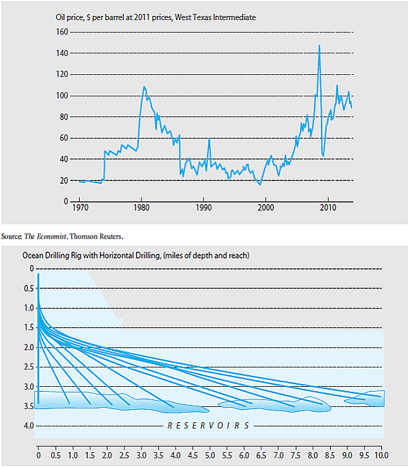
FIGURE Oil Price 1970-2012 and Drilling Rig with Horizontal Drilling
Question
In the Deep Creek Mining Company example described in this chapter (Table),
suppose again that labor is the variable input and capital is the fixed input. Specifically, assume that the firm owns a piece of equipment having a 500-bhp rating.
a. Complete the following table:
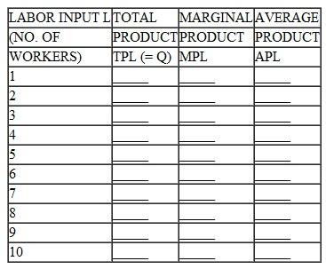 b. Plot the (i) total product, (ii) marginal product, and (iii) average product functions.
c. Determine the boundaries of the three stages of production.
Table TOTAL OUTPUT TABLE-DEEP CREEK MINING COMPANY
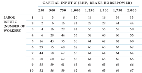
suppose again that labor is the variable input and capital is the fixed input. Specifically, assume that the firm owns a piece of equipment having a 500-bhp rating.
a. Complete the following table:
b. Plot the (i) total product, (ii) marginal product, and (iii) average product functions.c. Determine the boundaries of the three stages of production.
Table TOTAL OUTPUT TABLE-DEEP CREEK MINING COMPANY
Question
Question
Question
Question
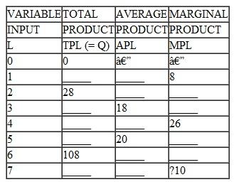
From your knowledge of the relationships among the various production functions,complete the following table:
Question
Question
The amount of fish caught per week on a trawler is a function of the crew size assigned to operate the boat. Based on past data, the following production schedule
was developed:
 a. Over what ranges of workers are there (i) increasing, (ii) constant, (iii) decreasing, and (iv) negative returns
b. How large a crew should be used if the trawler owner is interested in maximizing the total amount of fish caught
c. How large a crew should be used if the trawler owner is interested in maximizing the average amount of fish caught per person
was developed:
a. Over what ranges of workers are there (i) increasing, (ii) constant, (iii) decreasing, and (iv) negative returns b. How large a crew should be used if the trawler owner is interested in maximizing the total amount of fish caught
c. How large a crew should be used if the trawler owner is interested in maximizing the average amount of fish caught per person
Question

Unlock Deck
Sign up to unlock the cards in this deck!
Unlock Deck
Unlock Deck
1/19
Play
Full screen (f)
Deck 7: Production Economics
1
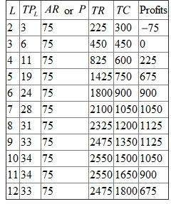
Consider Exercise again. Suppose the owner of the trawler can sell all the fishcaught for $75 per 100 pounds and can hire as many crew members as desired by paying them $150 per week. Assuming that the owner of the trawler is interested in maximizing profits, determine the optimal crew size.
Exercise
The amount of fish caught per week on a trawler is a function of the crew size assigned to operate the boat. Based on past data, the following production schedule was developed:
a. Over what ranges of workers are there (i) increasing, (ii) constant, (iii) decreasing, and (iv) negative returns
b. How large a crew should be used if the trawler owner is interested in maximizing the total amount of fish caught
c. How large a crew should be used if the trawler owner is interested in maximizing the average amount of fish caught per person
Exercise
The amount of fish caught per week on a trawler is a function of the crew size assigned to operate the boat. Based on past data, the following production schedule was developed:
a. Over what ranges of workers are there (i) increasing, (ii) constant, (iii) decreasing, and (iv) negative returns b. How large a crew should be used if the trawler owner is interested in maximizing the total amount of fish caught
c. How large a crew should be used if the trawler owner is interested in maximizing the average amount of fish caught per person
In the table below, we will calculate the total revenue, average revenue, total cost and the profits at each input level.
 The price
 is given as $75 per 100 pounds. The total revenue
 is obtained by multiplying price and total product. The
 at
at
 is
is
 . Similarly we can calculate the total revenue for other labor inputs. The total cost is obtained by multiplying quantity of labor and wage rate (the wage rate is given as $150 per worker). The total cost at
 is
is
 . Similarly we can calculate the total cost for other workers. The profits are obtained by subtracting total cost from total revenue.
We see that the profits gets maximized when labor is 8 or 9. The maximum profit is $1125.
The price is given as $75 per 100 pounds. The total revenue is obtained by multiplying price and total product. The at is . Similarly we can calculate the total revenue for other labor inputs. The total cost is obtained by multiplying quantity of labor and wage rate (the wage rate is given as $150 per worker). The total cost at is . Similarly we can calculate the total cost for other workers. The profits are obtained by subtracting total cost from total revenue.We see that the profits gets maximized when labor is 8 or 9. The maximum profit is $1125.
2
Determine whether this production function exhibits increasing, decreasing, or constant returns to scale. (Ignore the issue of statistical significance.)
The production function is:
 The general form of Cobb-Douglas production function is:
 The production function represents increasing returns to scale when
 , constant returns to scale when
 and decreasing returns to scale when
 .
.
This function shows decreasing returns to scale which means that if both capital and labor are increased by
 times, the output increases by less than
 times.
The degree of homogeiniety is
 .
.
The general form of Cobb-Douglas production function is: The production function represents increasing returns to scale when , constant returns to scale when and decreasing returns to scale when .This function shows decreasing returns to scale which means that if both capital and labor are increased by
times, the output increases by less than times.The degree of homogeiniety is
. 3
Consider the following short-run production function (where L = variable input, Q = output):Q = 6L3 0.4L3
a. Determine the marginal product function (MPL).
b. Determine the average product function (APL).
c. Find the value of L that maximizes Q.
d. Find the value of L at which the marginal product function takes on itsmaximum value.
e. Find the value of L at which the average product function takes on its maximumvalue.
The production function is given as:
 Where
Where
 is output or total product and
 is labor input.
(a)
The marginal product is the first derivative of total product.
 Thus the marginal product of labor is
 (b)
(b)
Average product is total product divided by labor input.
 Thus the average product of labor is
 (c)
(c)
The amount of labor at which the marginal product of labor is zero signifies maximum level of output production.

 Thus the value of L that maximizes Q is 10 units.
(d)
The amount of labor at which the first derivative of marginal product function is zero signifies its maximum value.
 Thus the value of L at which marginal product function takes on its maximum value is 5 units
(e)
The amount of labor at which the first derivative of average product function is zero signifies its maximum value.
 Thus the value of L at which marginal product function takes on its maximum value is 7.5 units
Where is output or total product and is labor input.(a)
The marginal product is the first derivative of total product.
Thus the marginal product of labor is (b)Average product is total product divided by labor input.
Thus the average product of labor is (c)The amount of labor at which the marginal product of labor is zero signifies maximum level of output production.
Thus the value of L that maximizes Q is 10 units. (d)
The amount of labor at which the first derivative of marginal product function is zero signifies its maximum value.
Thus the value of L at which marginal product function takes on its maximum value is 5 units (e)
The amount of labor at which the first derivative of average product function is zero signifies its maximum value.
Thus the value of L at which marginal product function takes on its maximum value is 7.5 units 4
Consider the following short-run production function (where L = variable input,Q = output):Q = 10L 0.5L2
Suppose that output can be sold for $10 per unit. Also assume that the firm can obtain as much of the variable input (L) as it needs at $20 per unit.
a. Determine the marginal revenue product function.
b. Determine the marginal factor cost function.
c. Determine the optimal value of L, given that the objective is to maximizeprofits
Unlock Deck
Unlock for access to all 19 flashcards in this deck.
Unlock Deck
k this deck
5
Suppose that a firm's production function is given by the following relationship:
Q = 2:5pffiLffiffiKffiffiffi ði:e:, Q = 2:5L:5K:5Þwhere Q = output
L = labor inputK = capital input
a. Determine the percentage increase in output if labor input is increased by 10 percent (assuming that capital input is held constant).
b. Determine the percentage increase in output if capital input is increased by 25 percent (assuming that labor input is held constant).
c. Determine the percentage increase in output if both labor and capital are increased by 20 percent.
Unlock Deck
Unlock for access to all 19 flashcards in this deck.
Unlock Deck
k this deck
6
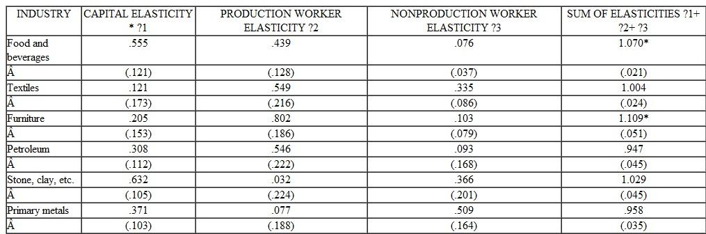
Based on the production function parameter estimates reported in Table:
a. Which industry (or industries) appears to exhibit decreasing returns to scale (Ignore the issue of statistical significance.)
b. Which industry comes closest to exhibiting constant returns to scale
c. In which industry will a given percentage increase in capital result in the largest percentage increase in output
d. In what industry will a given percentage increase in production workers result in the largest percentage increase in output
Table PRODUCTION ELASTICITIES FOR SEVERAL INDUSTRIES
Number in parentheses below each elasticity coefficient is the standard error.
*Significantly greater than 1.0 at the 0.05 level (one-tailed test).
Source: John R. Moroney, "Cobb-Douglas Production Functions and Returns to Scale in U.S. Manufacturing Industry," Western Economic Journal 6, no. 1 (December 1967), Table 1, p. 46.
a. Which industry (or industries) appears to exhibit decreasing returns to scale (Ignore the issue of statistical significance.)
b. Which industry comes closest to exhibiting constant returns to scale
c. In which industry will a given percentage increase in capital result in the largest percentage increase in output
d. In what industry will a given percentage increase in production workers result in the largest percentage increase in output
Table PRODUCTION ELASTICITIES FOR SEVERAL INDUSTRIES
Number in parentheses below each elasticity coefficient is the standard error.*Significantly greater than 1.0 at the 0.05 level (one-tailed test).
Source: John R. Moroney, "Cobb-Douglas Production Functions and Returns to Scale in U.S. Manufacturing Industry," Western Economic Journal 6, no. 1 (December 1967), Table 1, p. 46.
Unlock Deck
Unlock for access to all 19 flashcards in this deck.
Unlock Deck
k this deck
7
Consider the following Cobb-Douglas production function for the bus transportation system in a particular city:
where L = labor input in worker hours
F = fuel input in gallons
K = capital input in number of buses
Q = output measured in millions of bus miles
Suppose that the parameters ( , 1, 2, and 3) of this model were estimated using annual data for the past 25 years. The following results were obtained:
= 0.0012 1 = 0.45 2 = 0.20 3 = 0.30
a. Determine the (i) labor, (ii) fuel, and (iii) capital input production elasticities.
b. Suppose that labor input (worker hours) is increased by 2 percent next year (with the other inputs held constant). Determine the approximate percentage change in output.
c. Suppose that capital input (number of buses) is decreased by 3 percent next year (when certain older buses are taken out of service). Assuming that the other inputs are held constant, determine the approximate percentage changein output.
d. What type of returns to scale appears to characterize this bus transportation system (Ignore the issue of statistical significance.)
e. Discuss some of the methodological and measurement problems one might encounter in using time-series data to estimate the parameters of this model.
Unlock Deck
Unlock for access to all 19 flashcards in this deck.
Unlock Deck
k this deck
8
Extension of the Cobb-Douglas Production Function-The Cobb-Douglas production function (Equation) can be shown to be a special case of a larger class of linear homogeneous production functions having the following mathematical form: 11
where is an efficiency parameter that shows the output resulting from given quantities of inputs; is a distribution parameter (0 1) that indicates the division of factor income between capital and labor; is a substitution parameter that is a measure of substitutability of capital for labor (or vice versa) in the production process; and is a scale parameter ( 0) that indicates the type of returns to scale (increasing, constant, or decreasing). Show that when = 1, this function exhibits constant returns to scale. [Hint: Increase capital K and labor L each by a factor of , or K* = ( )K and L* = ( )L, and show that output Q also increases by a factor of , or Q* = ( )(Q).]
Equation
11 See R. G. Chambers, Applied Production Analysis (Cambridge: Cambridge University Press, 1988).
Unlock Deck
Unlock for access to all 19 flashcards in this deck.
Unlock Deck
k this deck
9
Lobo Lighting Corporation currently employs 100 unskilled laborers, 80 factorytechnicians, 30 skilled machinists, and 40 skilled electricians. Lobo feels that the marginal product of the last unskilled laborer is 400 lights per week, the marginal product of the last factory technician is 450 lights per week, the marginal product of the last skilled machinist is 550 lights per week, and the marginal product of the last skilled electrician is 600 lights per week. Unskilled laborers earn $400 per week, factory technicians earn $500 per week, machinists earn $700 per week, and electricians earn $750 per week. Is Lobo using the lowest cost combination of workers to produce its targeted output If not, what recommendations can you make to assist the company
Unlock Deck
Unlock for access to all 19 flashcards in this deck.
Unlock Deck
k this deck
10
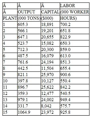
Estimate the Cobb-Douglas production function Q = L 1K 2 , where Q = output; L = labor input; K = capital input; and , 1, and 2 are the parameters to be estimated.
Unlock Deck
Unlock for access to all 19 flashcards in this deck.
Unlock Deck
k this deck
11
Figure shows the annual rate of crude oil extraction of the United States was basically unchanged 2002-2012. Not so for Saudi Arabia whose production increased 33%. Explain why with special attention to the price spike in mid-2008.
FIGURE Oil Price 1970-2012 and Drilling Rig with Horizontal Drilling
FIGURE Oil Price 1970-2012 and Drilling Rig with Horizontal Drilling
Unlock Deck
Unlock for access to all 19 flashcards in this deck.
Unlock Deck
k this deck
12
In the Deep Creek Mining Company example described in this chapter (Table),
suppose again that labor is the variable input and capital is the fixed input. Specifically, assume that the firm owns a piece of equipment having a 500-bhp rating.
a. Complete the following table:
b. Plot the (i) total product, (ii) marginal product, and (iii) average product functions.
c. Determine the boundaries of the three stages of production.
Table TOTAL OUTPUT TABLE-DEEP CREEK MINING COMPANY
suppose again that labor is the variable input and capital is the fixed input. Specifically, assume that the firm owns a piece of equipment having a 500-bhp rating.
a. Complete the following table:
b. Plot the (i) total product, (ii) marginal product, and (iii) average product functions.c. Determine the boundaries of the three stages of production.
Table TOTAL OUTPUT TABLE-DEEP CREEK MINING COMPANY
Unlock Deck
Unlock for access to all 19 flashcards in this deck.
Unlock Deck
k this deck
13
With interest rates at historic lows in the United States, what is the effect on the optimal rate of extraction for a Texas oilfield owner Explain the intuition that supports your answer.
Unlock Deck
Unlock for access to all 19 flashcards in this deck.
Unlock Deck
k this deck
14
Test whether the coefficients of capital and labor are statistically significant.
Unlock Deck
Unlock for access to all 19 flashcards in this deck.
Unlock Deck
k this deck
15
Explain the concept of maximum sustainable yield for a fishery. Is maximum sustainable yield the most efficient rate of harvest for a renewable natural resource Is it required to preserve biological diversity
Unlock Deck
Unlock for access to all 19 flashcards in this deck.
Unlock Deck
k this deck
16
From your knowledge of the relationships among the various production functions,complete the following table:
Unlock Deck
Unlock for access to all 19 flashcards in this deck.
Unlock Deck
k this deck
17
Determine the percentage of the variation in output that is "explained" by the regression equation.
Unlock Deck
Unlock for access to all 19 flashcards in this deck.
Unlock Deck
k this deck
18
The amount of fish caught per week on a trawler is a function of the crew size assigned to operate the boat. Based on past data, the following production schedule
was developed:
a. Over what ranges of workers are there (i) increasing, (ii) constant, (iii) decreasing, and (iv) negative returns
b. How large a crew should be used if the trawler owner is interested in maximizing the total amount of fish caught
c. How large a crew should be used if the trawler owner is interested in maximizing the average amount of fish caught per person
was developed:
a. Over what ranges of workers are there (i) increasing, (ii) constant, (iii) decreasing, and (iv) negative returns b. How large a crew should be used if the trawler owner is interested in maximizing the total amount of fish caught
c. How large a crew should be used if the trawler owner is interested in maximizing the average amount of fish caught per person
Unlock Deck
Unlock for access to all 19 flashcards in this deck.
Unlock Deck
k this deck
19
Determine the labor and capital estimated parameters, and give an economic interpretation of each value.
Unlock Deck
Unlock for access to all 19 flashcards in this deck.
Unlock Deck
k this deck
Unlock Deck
Unlock for access to all 19 flashcards in this deck.


