Deck 14: Introduction to Time Series Regression and Forecasting
Full screen (f)
Question
Question
The index of industrial production ( IP t ) is a monthly time series that measures the quantity of industrial commodities produced in a given month. This problem uses data on this index for the United States. All regressions are estimated over the sample period 1960:1 to 2000:12 (that is, January 1960 through December 2000). Let Y t = 1200 × In( IP t / IP t - 1 ).
a. The forecaster states that Y t shows the monthly percentage change in IP, measured in percentage points per annum. Is this correct Why
b. Suppose that a forecaster estimates the following AR(4) model for Y t.
Use this AR(4) to forecast the value of Y t in January 2001 using the following values of IP for August 2000 through December 2000:
 c. Worried about potential seasonal fluctuations in production, the forecaster adds Y t- 1 to the autoregression. The estimated coefficient on Y t-12 is -0.054 with a standard error of 0.053. Is this coefficient statistically significant
d. Worried about a potential break, she computes a QLR test (with 15% trimming) on the constant and AR coefficients in the AR(4) model. The resulting QLR statistic was 3.45. Is there evidence of a break Explain.
e. Worried that she might have included too few or too many lags in the model, the forecaster estimates AR( p ) models for p = 1,... ,6 over the same sample period. The sum of squared residuals from each of these estimated models is shown in the table. Use the BIC to estimate the number of lags that should be included in the autoregression. Do the results differ if you use the AIC
a. The forecaster states that Y t shows the monthly percentage change in IP, measured in percentage points per annum. Is this correct Why
b. Suppose that a forecaster estimates the following AR(4) model for Y t.
Use this AR(4) to forecast the value of Y t in January 2001 using the following values of IP for August 2000 through December 2000:
c. Worried about potential seasonal fluctuations in production, the forecaster adds Y t- 1 to the autoregression. The estimated coefficient on Y t-12 is -0.054 with a standard error of 0.053. Is this coefficient statistically significant d. Worried about a potential break, she computes a QLR test (with 15% trimming) on the constant and AR coefficients in the AR(4) model. The resulting QLR statistic was 3.45. Is there evidence of a break Explain.
e. Worried that she might have included too few or too many lags in the model, the forecaster estimates AR( p ) models for p = 1,... ,6 over the same sample period. The sum of squared residuals from each of these estimated models is shown in the table. Use the BIC to estimate the number of lags that should be included in the autoregression. Do the results differ if you use the AIC
Question
Question
Question
Question
Question
Question
Question
Prove the following results about conditional means, forecasts, and forecast errors:
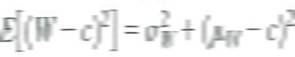
a. Let W be a random variable with mean and variance and let c be a constant. Show that
b. Consider the problem of forecasting Y t using data on Y t-1 , Y t-2 , …, Let f t-1 denote some forecast of Y t , where the subscript t - 1 on f t-1 indicates that the forecast is a function of data through date t- 1. Let be the conditional mean squared error of the forecast conditional on Y observed through date t - 1. Show that the conditional mean squared forecast error is minimized when
 , where
c. Let u t denote the error in Equation (14.14). Show that cov ( u t u t-j ) = 0 for; j 0.
a. Let W be a random variable with mean and variance and let c be a constant. Show that
b. Consider the problem of forecasting Y t using data on Y t-1 , Y t-2 , …, Let f t-1 denote some forecast of Y t , where the subscript t - 1 on f t-1 indicates that the forecast is a function of data through date t- 1. Let be the conditional mean squared error of the forecast conditional on Y observed through date t - 1. Show that the conditional mean squared forecast error is minimized when
, where c. Let u t denote the error in Equation (14.14). Show that cov ( u t u t-j ) = 0 for; j 0.
Question
Question
Question
Suppose that Y t is the monthly value of the number of new home construction projects started in the United States. Because of the weather, Y t has a pronounced seasonal pattern; for example, housing starts are low in January and high in June. Let
 , denote the average value of housing starts in January and denote the average values in the other months. Show that the values of can be estimated from the OLS regression
 where Feb t is a binary variable equal to 1 if t is February, Mar t is a binary variable
equal to 1 if t is March, and so forth. Show that ß 0 + ß 2 =
 and so forth.
, denote the average value of housing starts in January and denote the average values in the other months. Show that the values of can be estimated from the OLS regression where Feb t is a binary variable equal to 1 if t is February, Mar t is a binary variableequal to 1 if t is March, and so forth. Show that ß 0 + ß 2 =
and so forth. Question
The moving average model of order q has the form
 ,
,
where e t is a serially uncorrelated random variable with mean 0 and variance
 .
.
a. Show that E ( Y t ) = ß 0.
b. Show that the variance of Y t is var
 .
.
c. Show that for j q.
d. Suppose that q = 1. Derive the autocovariances for Y.
,where e t is a serially uncorrelated random variable with mean 0 and variance
. a. Show that E ( Y t ) = ß 0.
b. Show that the variance of Y t is var
.c. Show that for j q.
d. Suppose that q = 1. Derive the autocovariances for Y.
Question
Question
Question
Question

Unlock Deck
Sign up to unlock the cards in this deck!
Unlock Deck
Unlock Deck
1/17
Play
Full screen (f)
Deck 14: Introduction to Time Series Regression and Forecasting
1
Look at the plot of the logarithm of GDP for Japan in Figure 14.2c. Does this time series appear to be stationary Explain. Suppose that you calculated the first difference of this series. Would it appear to be stationary Explain.
The plot of the logarithm of the index of industrial production for Japan as shown in Fig 14.2C does not appear stationary. The most striking characteristic of the series is that it has an upward trend. That is, observations at the end of the sample are systematically larger than observations at the beginning. This suggests that the mean of the series is not constant, which would imply that it is not stationary.
Suppose we calculate the first difference of the series, which may look stationary, because first difference eliminates the large trend. However, the level of the first difference series is the slope of the plot. Looking at the figure, the slope is steeper in 1960-1975 than in 1976-1999, which in turn is steeper than in 2000-2013. Thus, it appears that there was a change in the mean of the first difference series. If there was a change in the population mean of the first difference series, then it too is non-stationary.
Suppose we calculate the first difference of the series, which may look stationary, because first difference eliminates the large trend. However, the level of the first difference series is the slope of the plot. Looking at the figure, the slope is steeper in 1960-1975 than in 1976-1999, which in turn is steeper than in 2000-2013. Thus, it appears that there was a change in the mean of the first difference series. If there was a change in the population mean of the first difference series, then it too is non-stationary.
2
The index of industrial production ( IP t ) is a monthly time series that measures the quantity of industrial commodities produced in a given month. This problem uses data on this index for the United States. All regressions are estimated over the sample period 1960:1 to 2000:12 (that is, January 1960 through December 2000). Let Y t = 1200 × In( IP t / IP t - 1 ).
a. The forecaster states that Y t shows the monthly percentage change in IP, measured in percentage points per annum. Is this correct Why
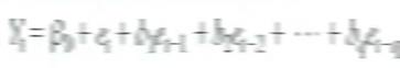
b. Suppose that a forecaster estimates the following AR(4) model for Y t.
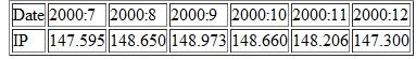
Use this AR(4) to forecast the value of Y t in January 2001 using the following values of IP for August 2000 through December 2000:
c. Worried about potential seasonal fluctuations in production, the forecaster adds Y t- 1 to the autoregression. The estimated coefficient on Y t-12 is -0.054 with a standard error of 0.053. Is this coefficient statistically significant
d. Worried about a potential break, she computes a QLR test (with 15% trimming) on the constant and AR coefficients in the AR(4) model. The resulting QLR statistic was 3.45. Is there evidence of a break Explain.
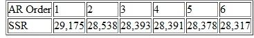
e. Worried that she might have included too few or too many lags in the model, the forecaster estimates AR( p ) models for p = 1,... ,6 over the same sample period. The sum of squared residuals from each of these estimated models is shown in the table. Use the BIC to estimate the number of lags that should be included in the autoregression. Do the results differ if you use the AIC
a. The forecaster states that Y t shows the monthly percentage change in IP, measured in percentage points per annum. Is this correct Why
b. Suppose that a forecaster estimates the following AR(4) model for Y t.
Use this AR(4) to forecast the value of Y t in January 2001 using the following values of IP for August 2000 through December 2000:
c. Worried about potential seasonal fluctuations in production, the forecaster adds Y t- 1 to the autoregression. The estimated coefficient on Y t-12 is -0.054 with a standard error of 0.053. Is this coefficient statistically significant d. Worried about a potential break, she computes a QLR test (with 15% trimming) on the constant and AR coefficients in the AR(4) model. The resulting QLR statistic was 3.45. Is there evidence of a break Explain.
e. Worried that she might have included too few or too many lags in the model, the forecaster estimates AR( p ) models for p = 1,... ,6 over the same sample period. The sum of squared residuals from each of these estimated models is shown in the table. Use the BIC to estimate the number of lags that should be included in the autoregression. Do the results differ if you use the AIC
IIP is a monthly time series that is helpful in measuring number of manufacturing goods and services made in certain period of time. This problem uses the data of United States, estimated over time period of 1986:M1 to 2013:M12.
Equation is given as,
 (a)
(a)
Yes, the given part is right. The proportion of IP on monthly basis is
 , that can be done through
 , in the case of slight variations. Altering the above part to annual change leads to
 .
.
(b)
The values for variable Y is being provided as follows:
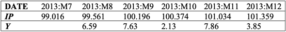 The projected value of
 for the month of January is provided as follows:
 (c)
(c)
The value of t- statistic for
 is provided as,
 Its total value is smaller than 1.96, implying that the particular factor is not substantial with the 5 percent level of significance.
(d)
For QLR test, a total of 5 coefficients are acceptable to break. Equated with critical values of q = 5 in the table 14.5 of this textbook, QLR statistic 3.94 is greater than 10 percent critical significant (3.59) and 5 percent critical value (3.66) but smaller than 1% critical value (4.53). Therefore, there is strong evidence of break at 5% and 10% level of significance.
(e).
The BIC is calculated by the formula:
 The AIC is calculated by the formula:
 Here T = 324 (27 years, 12 months per year)
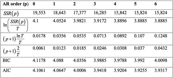 The BIC is least in the case where p = 4. Consequently, BIC approximation of lag length is 4.
The AIC is least in case of p = 4. So, AIC estimate of lag length is also 4.
Therefore, the results did not differ if the AIC is used.
Equation is given as,
(a) Yes, the given part is right. The proportion of IP on monthly basis is
, that can be done through , in the case of slight variations. Altering the above part to annual change leads to .(b)
The values for variable Y is being provided as follows:
The projected value of for the month of January is provided as follows: (c) The value of t- statistic for
is provided as, Its total value is smaller than 1.96, implying that the particular factor is not substantial with the 5 percent level of significance. (d)
For QLR test, a total of 5 coefficients are acceptable to break. Equated with critical values of q = 5 in the table 14.5 of this textbook, QLR statistic 3.94 is greater than 10 percent critical significant (3.59) and 5 percent critical value (3.66) but smaller than 1% critical value (4.53). Therefore, there is strong evidence of break at 5% and 10% level of significance.
(e).
The BIC is calculated by the formula:
The AIC is calculated by the formula: Here T = 324 (27 years, 12 months per year) The BIC is least in the case where p = 4. Consequently, BIC approximation of lag length is 4. The AIC is least in case of p = 4. So, AIC estimate of lag length is also 4.
Therefore, the results did not differ if the AIC is used.
3
On the textbook Web site Mww.pearsonhighered.coni/stock_watson, you will find a data file USMacro_Quarterly that contains quarterly data on several macroeconomic series for the United States; the data are described in the file USMacro_Description. Compute Y t = ln( GDP t ; ) , the logarithm of real GDP, and Y t the quarterly growth rate of GDP. In Empirical Exercises 14.1 through 14.6, use the sample period 1955:1-2009:4 (where data before 1955 may be used, as necessary, as initial values for lags in regressions).
a. Estimate an AR(1) model for A Y,. What is the estimated AR(1) coefficient Is the coefficient statistically significantly different from zero Construct a 95% confidence interval for the population AR(1) coefficient.
b. Estimate an AR(2) model for Y t. Is the AR(2) coefficient statistically significantly different from zero Is this model preferred to the AR(1) model
c. Estimate AR(3) and AR(4) models. (/) Using the estimated AR(1) through AR(4) models, use BIC to choose the number of lags in the AR model, (ii) How many lags does AIC choose
NO ANSWER
4
Many financial economists believe that the random walk model is a good description of the logarithm of stock prices. It implies that the percentage changes in stock prices are unforecastable. A financial analyst claims to have a new model that makes better predictions than the random walk model. Explain how you would examine the analyst's claim that his model is superior.
Unlock Deck
Unlock for access to all 17 flashcards in this deck.
Unlock Deck
k this deck
5
Using the same data as in Exercise 14.2, a researcher tests for a stochastic trend in In (IP t ) using the following regression:
where the standard errors shown in parentheses are computed using the homoskedasticity-only formula and the regressor "t" is a linear time trend.
a. Use the ADF statistic to test for a stochastic trend (unit root) in In (IP).
b. Do these results support the specification used in Exercise 14.2 Explain.
Unlock Deck
Unlock for access to all 17 flashcards in this deck.
Unlock Deck
k this deck
6
A researcher estimates an AR(1) with an intercept and finds that the OLS estimate of ß 1 is 0.95, with a standard error of 0.02. Does a 95% confidence interval include ß 1 = 1 Explain.
Unlock Deck
Unlock for access to all 17 flashcards in this deck.
Unlock Deck
k this deck
7
The forecaster in Exercise 14.2 augments her AR(4) model for IP growth to include four lagged values of R t , where R t is the interest rate on three-month U.S. Treasury bills (measured in percentage points at an annual rate).
a. The Granger-causality F -statistic on the four lags of R t is 2.35. Do interest rates help to predict IP growth Explain.
b. The researcher also regresses R t on a constant, four lags of R t and four lags of IP growth. The resulting Granger-causality E-statistic on the four lags of IP growth is 2.87. Does IP growth help to predict interest rates Explain.
Unlock Deck
Unlock for access to all 17 flashcards in this deck.
Unlock Deck
k this deck
8
Suppose that you suspected that the intercept in Equation (14.17) changed in 1992:1. How would you modify the equation to incorporate this change How would you test for a change in the intercept How would you test for a change in the intercept if you did not know the date of the change
Unlock Deck
Unlock for access to all 17 flashcards in this deck.
Unlock Deck
k this deck
9
Prove the following results about conditional means, forecasts, and forecast errors:
a. Let W be a random variable with mean and variance and let c be a constant. Show that
b. Consider the problem of forecasting Y t using data on Y t-1 , Y t-2 , …, Let f t-1 denote some forecast of Y t , where the subscript t - 1 on f t-1 indicates that the forecast is a function of data through date t- 1. Let be the conditional mean squared error of the forecast conditional on Y observed through date t - 1. Show that the conditional mean squared forecast error is minimized when
, where
c. Let u t denote the error in Equation (14.14). Show that cov ( u t u t-j ) = 0 for; j 0.
a. Let W be a random variable with mean and variance and let c be a constant. Show that
b. Consider the problem of forecasting Y t using data on Y t-1 , Y t-2 , …, Let f t-1 denote some forecast of Y t , where the subscript t - 1 on f t-1 indicates that the forecast is a function of data through date t- 1. Let be the conditional mean squared error of the forecast conditional on Y observed through date t - 1. Show that the conditional mean squared forecast error is minimized when
, where c. Let u t denote the error in Equation (14.14). Show that cov ( u t u t-j ) = 0 for; j 0.
Unlock Deck
Unlock for access to all 17 flashcards in this deck.
Unlock Deck
k this deck
10
In this exercise you will conduct a Monte Carlo experiment that studies the phenomenon of spurious regression discussed in Section 14.6. In a Monte Carlo study, artificial data are generated using a computer, and then these artificial data are used to calculate the statistics being studied. This makes it possible to compute the distribution of statistics for known models when mathematical expressions for those distributions are complicated (as they are here) or even unknown. In this exercise, you will generate data so that two series, Y t and X t, are independently distributed random walks. The specific steps are as follows:
i. Use your computer to generate a sequence of T = 100 i.i.d. standard normal random variables. Call these variables e 1, e 2 ,..., e 100. Set Y t = e 1 and Y t = Y t-1 + e t for t = 2,3,..., 100.
ii. Use your computer to ge nerate a new sequence, a 1, a 2 , …, a 100 , of T= 100 i.i.d. standard normal random variables. Set X 1 = a 1 and X t = X t- 1 + a t for t = 2, 3,..., 100.
iii. Regress Y t onto a constant and X t Compute the OLS estimator, the regression R 2 , and the (homoskedastic-only) t -statistic testing the null hypothesis that ß 1 (the coefficient on X t ) is zero.
Use this algorithm to answer the following questions:
a. Run the algorithm (i) through (iii) once. Use the t -statistic from (iii) to test the null hypothesis that ß 1 = 0 using the usual 5% critical value of 1.96. What is the R 2 of your regression
b. Repeat (a) 1000 times, saving each value of R 2 and the t -statistic. Construct a histogram of the R 2 and t -statistic. What are the 5%, 50%, and 95% percentiles of the distributions of the R 2 and the t -statistic In what fraction of your 1000 simulated data sets does the t -statistic exceed 1.96 in absolute value
c. Repeat (b) for different numbers of observations, for example, T = 50 and T = 200. As the sample size increases, does the fraction of times that you reject the null hypothesis approach 5%, as it should because you have generated Y and X to be independently distributed Does this fraction seem to approach some other limit as T gets large What is that limit
Unlock Deck
Unlock for access to all 17 flashcards in this deck.
Unlock Deck
k this deck
11
Suppose that Y t follows the stationary AR(1) model Y t = 2.5 + 0.7 Y t-1 + u t , where u t is i.i.d. with E ( u t ) = 0 and var( u t ) = 9.
a. Compute the mean and variance of Y t.
b. Compute the first two autocovariances of Y t.
c. Compute the first two autocorrelations of Y t.
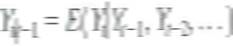
d. Suppose that Y T = 102.3. Compute Y r+1 | T = E ( Y T+1 \Y T , Y t- 1,...).
a. Compute the mean and variance of Y t.
b. Compute the first two autocovariances of Y t.
c. Compute the first two autocorrelations of Y t.
d. Suppose that Y T = 102.3. Compute Y r+1 | T = E ( Y T+1 \Y T , Y t- 1,...).
Unlock Deck
Unlock for access to all 17 flashcards in this deck.
Unlock Deck
k this deck
12
Suppose that Y t is the monthly value of the number of new home construction projects started in the United States. Because of the weather, Y t has a pronounced seasonal pattern; for example, housing starts are low in January and high in June. Let
, denote the average value of housing starts in January and denote the average values in the other months. Show that the values of can be estimated from the OLS regression
where Feb t is a binary variable equal to 1 if t is February, Mar t is a binary variable
equal to 1 if t is March, and so forth. Show that ß 0 + ß 2 =
and so forth.
, denote the average value of housing starts in January and denote the average values in the other months. Show that the values of can be estimated from the OLS regression where Feb t is a binary variable equal to 1 if t is February, Mar t is a binary variableequal to 1 if t is March, and so forth. Show that ß 0 + ß 2 =
and so forth. Unlock Deck
Unlock for access to all 17 flashcards in this deck.
Unlock Deck
k this deck
13
The moving average model of order q has the form
,
where e t is a serially uncorrelated random variable with mean 0 and variance
.
a. Show that E ( Y t ) = ß 0.
b. Show that the variance of Y t is var
.
c. Show that for j q.
d. Suppose that q = 1. Derive the autocovariances for Y.
,where e t is a serially uncorrelated random variable with mean 0 and variance
. a. Show that E ( Y t ) = ß 0.
b. Show that the variance of Y t is var
.c. Show that for j q.
d. Suppose that q = 1. Derive the autocovariances for Y.
Unlock Deck
Unlock for access to all 17 flashcards in this deck.
Unlock Deck
k this deck
14
A researcher carries out a QLR test using 25% trimming, and there are q = 5 restrictions. Answer the following questions using the values in Table 14.6 ("Critical Values of the QLR Statistic with 15% Trimming") and Appendix Table 4 ("Critical Values of the F m Distribution").
a. The QLR F -statistic is 4.2. Should the researcher reject the null hypothesis at the 5 % level
b. The QLR F -statistic is 2.1. Should the researcher reject the null hypothesis at the 5 % level
c. The QLR F -statistic is 3.5. Should the researcher reject the null hypothesis at the 5% level
a. The QLR F -statistic is 4.2. Should the researcher reject the null hypothesis at the 5 % level
b. The QLR F -statistic is 2.1. Should the researcher reject the null hypothesis at the 5 % level
c. The QLR F -statistic is 3.5. Should the researcher reject the null hypothesis at the 5% level
Unlock Deck
Unlock for access to all 17 flashcards in this deck.
Unlock Deck
k this deck
15
Consider the AR(1) model Y t = ß 0 + ß 1 Y t - 1 + u t. Suppose that the process is stationary.
a. Show that E ( Y t ) = E ( Y t - 1 ).
b. Show that E(Y,) = ß 0 /(l - ß 1 ).
a. Show that E ( Y t ) = E ( Y t - 1 ).
b. Show that E(Y,) = ß 0 /(l - ß 1 ).
Unlock Deck
Unlock for access to all 17 flashcards in this deck.
Unlock Deck
k this deck
16
Suppose that Y t follows the AR(1) model Y t = ß 0 + ß 1 Y t -1 + u 1.
a. Show that Y t follows an AR(2) model.
b. Derive the AR(2) coefficients for Y t as a function of ß 0 and ß 1.
a. Show that Y t follows an AR(2) model.
b. Derive the AR(2) coefficients for Y t as a function of ß 0 and ß 1.
Unlock Deck
Unlock for access to all 17 flashcards in this deck.
Unlock Deck
k this deck
17
On the textbook Web site Mww.pearsonhighered.coni/stock_watson, you will find a data file USMacro_Quarterly that contains quarterly data on several macroeconomic series for the United States; the data are described in the file USMacro_Description. Compute Y t = ln( GDP t ; ) , the logarithm of real GDP, and Y t the quarterly growth rate of GDP. In Empirical Exercises 14.1 through 14.6, use the sample period 1955:1-2009:4 (where data before 1955 may be used, as necessary, as initial values for lags in regressions).
a. Estimate the mean of Y t.
b. Express the mean growth rate in percentage points at an annual rate.
c. Estimate the standard deviation of Y t. Express your answer in percentage points at an annual rate.
d. Estimate the first four autocorrelations of Y t.. What are the units of the autocorrelations (quarterly rates of growth, percentage points at an annual rate, or no units at all)
Unlock Deck
Unlock for access to all 17 flashcards in this deck.
Unlock Deck
k this deck
Unlock Deck
Unlock for access to all 17 flashcards in this deck.


