Deck 18: The Theory of Multiple Regression
Full screen (f)
Question
Question
Question
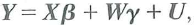
Show that
 is the efficient GMM estimator-that is, that
 Equation (18.66) is the solution to Equation (18.65).
b. Show that
c. Show that
is the efficient GMM estimator-that is, that Equation (18.66) is the solution to Equation (18.65).b. Show that
c. Show that
Question
Question
Consider the problem of minimizing the sum of squared residuals subject to the constraint that Rb = r, where R is q × ( k + 1) with rank cj. Let
 be the value of b that solves the constrained minimization problem.
a. Show that the Lagrangian for the minimization problem is L(b , ) = ( Y- Xb ) ' ( Y-Xb ) + ' ( Rb - r ), where is a q × 1 vector of Lagrange multipliers.
b. Show that
c. Show that

d. Show that F in Equation (18.36) is equivalent to the homoskeskasticity-only F -statistic in Equation (7.13).
be the value of b that solves the constrained minimization problem.a. Show that the Lagrangian for the minimization problem is L(b , ) = ( Y- Xb ) ' ( Y-Xb ) + ' ( Rb - r ), where is a q × 1 vector of Lagrange multipliers.
b. Show that
c. Show that
d. Show that F in Equation (18.36) is equivalent to the homoskeskasticity-only F -statistic in Equation (7.13).
Question
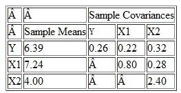
Suppose that a sample of n = 20 households has the sample means and sample covariances below for a dependent variable and two regressors:
 a. Calculate the OLS estimates of ß 0 , ß h and ß 2 Calculate s 2 u ,. Calculate the R 2 of the regression.
b. Suppose that all six assumptions in Key Concept 18.1 hold. Test the hypothesis that ß 1 = 0 at the 5% significance level.
a. Calculate the OLS estimates of ß 0 , ß h and ß 2 Calculate s 2 u ,. Calculate the R 2 of the regression.b. Suppose that all six assumptions in Key Concept 18.1 hold. Test the hypothesis that ß 1 = 0 at the 5% significance level.
Question
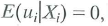
Consider the regression model Y = Xß + U. Partition X as [ X 1 X 2 ] and ß as
![Consider the regression model Y = Xß + U. Partition X as [ X 1 X 2 ] and ß as where X 1 has k 1 columns and X 2 has k 2 columns. Suppose that Let a. Show that b. Consider the regression described in Equation (12.17). Let W = [1 W 1 W 2 … W r ], where 1 is an n × 1 vector of ones, W l is the n X 1 vector with i th element W 1 i and so forth. Let denote the vector of two stage least squares residuals. i. Show that ii. Show that the method for computing the J -statistic described in Key Concept 12.6 (using a homoskedasiticity-only F-statistic) and the formula in Equation (18.63) produce the same value for the J -statistic. [Hint: Use the results in (a), (b, i), and Exercise 18.13.]<div style=padding-top: 35px>](https://d2lvgg3v3hfg70.cloudfront.net/SM2685/11eb817c_781a_ec42_84e6_c944d1fd1c62_SM2685_11.jpg) where X 1 has k 1 columns and X 2 has k 2 columns. Suppose that
where X 1 has k 1 columns and X 2 has k 2 columns. Suppose that
![Consider the regression model Y = Xß + U. Partition X as [ X 1 X 2 ] and ß as where X 1 has k 1 columns and X 2 has k 2 columns. Suppose that Let a. Show that b. Consider the regression described in Equation (12.17). Let W = [1 W 1 W 2 … W r ], where 1 is an n × 1 vector of ones, W l is the n X 1 vector with i th element W 1 i and so forth. Let denote the vector of two stage least squares residuals. i. Show that ii. Show that the method for computing the J -statistic described in Key Concept 12.6 (using a homoskedasiticity-only F-statistic) and the formula in Equation (18.63) produce the same value for the J -statistic. [Hint: Use the results in (a), (b, i), and Exercise 18.13.]<div style=padding-top: 35px>](https://d2lvgg3v3hfg70.cloudfront.net/SM2685/11eb817c_781a_ec43_84e6_81fb05f143b0_SM2685_11.jpg) Let
Let
![Consider the regression model Y = Xß + U. Partition X as [ X 1 X 2 ] and ß as where X 1 has k 1 columns and X 2 has k 2 columns. Suppose that Let a. Show that b. Consider the regression described in Equation (12.17). Let W = [1 W 1 W 2 … W r ], where 1 is an n × 1 vector of ones, W l is the n X 1 vector with i th element W 1 i and so forth. Let denote the vector of two stage least squares residuals. i. Show that ii. Show that the method for computing the J -statistic described in Key Concept 12.6 (using a homoskedasiticity-only F-statistic) and the formula in Equation (18.63) produce the same value for the J -statistic. [Hint: Use the results in (a), (b, i), and Exercise 18.13.]<div style=padding-top: 35px>](https://d2lvgg3v3hfg70.cloudfront.net/SM2685/11eb817c_781a_ec44_84e6_99bdafe13e64_SM2685_11.jpg)
a. Show that
![Consider the regression model Y = Xß + U. Partition X as [ X 1 X 2 ] and ß as where X 1 has k 1 columns and X 2 has k 2 columns. Suppose that Let a. Show that b. Consider the regression described in Equation (12.17). Let W = [1 W 1 W 2 … W r ], where 1 is an n × 1 vector of ones, W l is the n X 1 vector with i th element W 1 i and so forth. Let denote the vector of two stage least squares residuals. i. Show that ii. Show that the method for computing the J -statistic described in Key Concept 12.6 (using a homoskedasiticity-only F-statistic) and the formula in Equation (18.63) produce the same value for the J -statistic. [Hint: Use the results in (a), (b, i), and Exercise 18.13.]<div style=padding-top: 35px>](https://d2lvgg3v3hfg70.cloudfront.net/SM2685/11eb817c_781a_ec45_84e6_6d7d2a6ec3fd_SM2685_00.jpg)
b. Consider the regression described in Equation (12.17). Let W = [1 W 1 W 2 … W r ], where 1 is an n × 1 vector of ones, W l is the n X 1 vector with i th element W 1 i and so forth. Let
![Consider the regression model Y = Xß + U. Partition X as [ X 1 X 2 ] and ß as where X 1 has k 1 columns and X 2 has k 2 columns. Suppose that Let a. Show that b. Consider the regression described in Equation (12.17). Let W = [1 W 1 W 2 … W r ], where 1 is an n × 1 vector of ones, W l is the n X 1 vector with i th element W 1 i and so forth. Let denote the vector of two stage least squares residuals. i. Show that ii. Show that the method for computing the J -statistic described in Key Concept 12.6 (using a homoskedasiticity-only F-statistic) and the formula in Equation (18.63) produce the same value for the J -statistic. [Hint: Use the results in (a), (b, i), and Exercise 18.13.]<div style=padding-top: 35px>](https://d2lvgg3v3hfg70.cloudfront.net/SM2685/11eb817c_781b_1356_84e6_3f4dd12d3463_SM2685_11.jpg) denote the vector of two stage least squares residuals.
denote the vector of two stage least squares residuals.
i. Show that
![Consider the regression model Y = Xß + U. Partition X as [ X 1 X 2 ] and ß as where X 1 has k 1 columns and X 2 has k 2 columns. Suppose that Let a. Show that b. Consider the regression described in Equation (12.17). Let W = [1 W 1 W 2 … W r ], where 1 is an n × 1 vector of ones, W l is the n X 1 vector with i th element W 1 i and so forth. Let denote the vector of two stage least squares residuals. i. Show that ii. Show that the method for computing the J -statistic described in Key Concept 12.6 (using a homoskedasiticity-only F-statistic) and the formula in Equation (18.63) produce the same value for the J -statistic. [Hint: Use the results in (a), (b, i), and Exercise 18.13.]<div style=padding-top: 35px>](https://d2lvgg3v3hfg70.cloudfront.net/SM2685/11eb817c_781b_1357_84e6_0d40d73367c8_SM2685_11.jpg)
ii. Show that the method for computing the J -statistic described in Key Concept 12.6 (using a homoskedasiticity-only F-statistic) and the formula in Equation (18.63) produce the same value for the J -statistic. [Hint: Use the results in (a), (b, i), and Exercise 18.13.]
where X 1 has k 1 columns and X 2 has k 2 columns. Suppose that Let a. Show that
b. Consider the regression described in Equation (12.17). Let W = [1 W 1 W 2 … W r ], where 1 is an n × 1 vector of ones, W l is the n X 1 vector with i th element W 1 i and so forth. Let
denote the vector of two stage least squares residuals.i. Show that
ii. Show that the method for computing the J -statistic described in Key Concept 12.6 (using a homoskedasiticity-only F-statistic) and the formula in Equation (18.63) produce the same value for the J -statistic. [Hint: Use the results in (a), (b, i), and Exercise 18.13.]
Question
Question
(Consistency of clustered standard errors.) Consider the panel data model
 where all variables are scalars. Assume that Assumption #1, #2, and #4 in Key Concept 10.3 hold and strengthen Assumption #3 so that X it and u it have eight nonzero finite moments. Let M = I T T 1 , where is a T × 1 vector ones, Also let Y i = ( Y i 1 · Y i 2 … Y iT ) , X i = ( X i 1 X i 2 … X iT ) , u i = ( u i 1 u i 2 … u iT ) ,
 , and
, and
 . For the asymptotic calculations in this problem, suppose that T is fixed and n
where all variables are scalars. Assume that Assumption #1, #2, and #4 in Key Concept 10.3 hold and strengthen Assumption #3 so that X it and u it have eight nonzero finite moments. Let M = I T T 1 , where is a T × 1 vector ones, Also let Y i = ( Y i 1 · Y i 2 … Y iT ) , X i = ( X i 1 X i 2 … X iT ) , u i = ( u i 1 u i 2 … u iT ) , , and . For the asymptotic calculations in this problem, suppose that T is fixed and n Question
Let W be an m × 1 vector with covariance matrix
 where
where
 is finite and positive definite. Let c be a nonrandom m × 1 vector, and let

a. Show that var
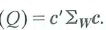
b. Suppose that c 0 m Show that 0 var(Q) .
where is finite and positive definite. Let c be a nonrandom m × 1 vector, and let a. Show that var
b. Suppose that c 0 m Show that 0 var(Q) .
Question
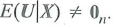
This exercise takes up the problem of missing data discussed in Section 9.2. Consider the regression model
![This exercise takes up the problem of missing data discussed in Section 9.2. Consider the regression model where all variables are scalars and the constant term/intercept is omitted for convenience. a. Suppose that the least assumptions in Key Concept 4.3 are satisfied. Show that the least squares estimator of ß is unbiased and consistent. b. Now suppose that some of the observations are missing. Let I i , denote a binary random variable that indicates the nonmissing observations; that is, I i = 1 if observation i is not missing and I i = 0 if observation i is missing. Assume that are i.i.d. i. Show that the OLS estimator can be written as ii. Suppose that data are missing completely at random in the sense that where p is a constant. Show that is unbiased and consistent. iii. Suppose that the probability that the i th observation is missing depends of X i but not on u i ; that is, Show that is unbiased and consistent. iv. Suppose that the probability that the i th observation is missing depends on both X i and u i ; that is, Is unbiased Is consistent Explain. c. Suppose that ß = 1 and that X i and u i are mutually independent standard normal random variables [so that both X t and iq are distributed N (0,1)]. Suppose that I i = 1 when Y i 0, but I i = 0 when Y i 0. Is unbiased Is consistent Explain.<div style=padding-top: 35px>](https://d2lvgg3v3hfg70.cloudfront.net/SM2685/11eb817c_781b_aeb2_84e6_45e8bfc9e6da_SM2685_11.jpg) where all variables are scalars and the constant term/intercept is omitted for convenience.
where all variables are scalars and the constant term/intercept is omitted for convenience.
a. Suppose that the least assumptions in Key Concept 4.3 are satisfied. Show that the least squares estimator of ß is unbiased and consistent.
b. Now suppose that some of the observations are missing. Let I i , denote a binary random variable that indicates the nonmissing observations; that is, I i = 1 if observation i is not missing and I i = 0 if observation i is missing. Assume that
![This exercise takes up the problem of missing data discussed in Section 9.2. Consider the regression model where all variables are scalars and the constant term/intercept is omitted for convenience. a. Suppose that the least assumptions in Key Concept 4.3 are satisfied. Show that the least squares estimator of ß is unbiased and consistent. b. Now suppose that some of the observations are missing. Let I i , denote a binary random variable that indicates the nonmissing observations; that is, I i = 1 if observation i is not missing and I i = 0 if observation i is missing. Assume that are i.i.d. i. Show that the OLS estimator can be written as ii. Suppose that data are missing completely at random in the sense that where p is a constant. Show that is unbiased and consistent. iii. Suppose that the probability that the i th observation is missing depends of X i but not on u i ; that is, Show that is unbiased and consistent. iv. Suppose that the probability that the i th observation is missing depends on both X i and u i ; that is, Is unbiased Is consistent Explain. c. Suppose that ß = 1 and that X i and u i are mutually independent standard normal random variables [so that both X t and iq are distributed N (0,1)]. Suppose that I i = 1 when Y i 0, but I i = 0 when Y i 0. Is unbiased Is consistent Explain.<div style=padding-top: 35px>](https://d2lvgg3v3hfg70.cloudfront.net/SM2685/11eb817c_781b_aeb3_84e6_1b2ffeacc0c0_SM2685_00.jpg) are i.i.d.
are i.i.d.
i. Show that the OLS estimator can be written as
![This exercise takes up the problem of missing data discussed in Section 9.2. Consider the regression model where all variables are scalars and the constant term/intercept is omitted for convenience. a. Suppose that the least assumptions in Key Concept 4.3 are satisfied. Show that the least squares estimator of ß is unbiased and consistent. b. Now suppose that some of the observations are missing. Let I i , denote a binary random variable that indicates the nonmissing observations; that is, I i = 1 if observation i is not missing and I i = 0 if observation i is missing. Assume that are i.i.d. i. Show that the OLS estimator can be written as ii. Suppose that data are missing completely at random in the sense that where p is a constant. Show that is unbiased and consistent. iii. Suppose that the probability that the i th observation is missing depends of X i but not on u i ; that is, Show that is unbiased and consistent. iv. Suppose that the probability that the i th observation is missing depends on both X i and u i ; that is, Is unbiased Is consistent Explain. c. Suppose that ß = 1 and that X i and u i are mutually independent standard normal random variables [so that both X t and iq are distributed N (0,1)]. Suppose that I i = 1 when Y i 0, but I i = 0 when Y i 0. Is unbiased Is consistent Explain.<div style=padding-top: 35px>](https://d2lvgg3v3hfg70.cloudfront.net/SM2685/11eb817c_781b_aeb4_84e6_352acfa5cf12_SM2685_00.jpg)
ii. Suppose that data are "missing completely at random" in the sense that
![This exercise takes up the problem of missing data discussed in Section 9.2. Consider the regression model where all variables are scalars and the constant term/intercept is omitted for convenience. a. Suppose that the least assumptions in Key Concept 4.3 are satisfied. Show that the least squares estimator of ß is unbiased and consistent. b. Now suppose that some of the observations are missing. Let I i , denote a binary random variable that indicates the nonmissing observations; that is, I i = 1 if observation i is not missing and I i = 0 if observation i is missing. Assume that are i.i.d. i. Show that the OLS estimator can be written as ii. Suppose that data are missing completely at random in the sense that where p is a constant. Show that is unbiased and consistent. iii. Suppose that the probability that the i th observation is missing depends of X i but not on u i ; that is, Show that is unbiased and consistent. iv. Suppose that the probability that the i th observation is missing depends on both X i and u i ; that is, Is unbiased Is consistent Explain. c. Suppose that ß = 1 and that X i and u i are mutually independent standard normal random variables [so that both X t and iq are distributed N (0,1)]. Suppose that I i = 1 when Y i 0, but I i = 0 when Y i 0. Is unbiased Is consistent Explain.<div style=padding-top: 35px>](https://d2lvgg3v3hfg70.cloudfront.net/SM2685/11eb817c_781b_d5c5_84e6_efd087fff819_SM2685_00.jpg) where p is a constant. Show that
where p is a constant. Show that
![This exercise takes up the problem of missing data discussed in Section 9.2. Consider the regression model where all variables are scalars and the constant term/intercept is omitted for convenience. a. Suppose that the least assumptions in Key Concept 4.3 are satisfied. Show that the least squares estimator of ß is unbiased and consistent. b. Now suppose that some of the observations are missing. Let I i , denote a binary random variable that indicates the nonmissing observations; that is, I i = 1 if observation i is not missing and I i = 0 if observation i is missing. Assume that are i.i.d. i. Show that the OLS estimator can be written as ii. Suppose that data are missing completely at random in the sense that where p is a constant. Show that is unbiased and consistent. iii. Suppose that the probability that the i th observation is missing depends of X i but not on u i ; that is, Show that is unbiased and consistent. iv. Suppose that the probability that the i th observation is missing depends on both X i and u i ; that is, Is unbiased Is consistent Explain. c. Suppose that ß = 1 and that X i and u i are mutually independent standard normal random variables [so that both X t and iq are distributed N (0,1)]. Suppose that I i = 1 when Y i 0, but I i = 0 when Y i 0. Is unbiased Is consistent Explain.<div style=padding-top: 35px>](https://d2lvgg3v3hfg70.cloudfront.net/SM2685/11eb817c_781b_d5c6_84e6_2d52340a42ec_SM2685_11.jpg) is unbiased and consistent.
is unbiased and consistent.
iii. Suppose that the probability that the i th observation is missing depends of X i but not on u i ; that is,
![This exercise takes up the problem of missing data discussed in Section 9.2. Consider the regression model where all variables are scalars and the constant term/intercept is omitted for convenience. a. Suppose that the least assumptions in Key Concept 4.3 are satisfied. Show that the least squares estimator of ß is unbiased and consistent. b. Now suppose that some of the observations are missing. Let I i , denote a binary random variable that indicates the nonmissing observations; that is, I i = 1 if observation i is not missing and I i = 0 if observation i is missing. Assume that are i.i.d. i. Show that the OLS estimator can be written as ii. Suppose that data are missing completely at random in the sense that where p is a constant. Show that is unbiased and consistent. iii. Suppose that the probability that the i th observation is missing depends of X i but not on u i ; that is, Show that is unbiased and consistent. iv. Suppose that the probability that the i th observation is missing depends on both X i and u i ; that is, Is unbiased Is consistent Explain. c. Suppose that ß = 1 and that X i and u i are mutually independent standard normal random variables [so that both X t and iq are distributed N (0,1)]. Suppose that I i = 1 when Y i 0, but I i = 0 when Y i 0. Is unbiased Is consistent Explain.<div style=padding-top: 35px>](https://d2lvgg3v3hfg70.cloudfront.net/SM2685/11eb817c_781b_d5c7_84e6_0faecf992bad_SM2685_11.jpg) Show that
Show that
![This exercise takes up the problem of missing data discussed in Section 9.2. Consider the regression model where all variables are scalars and the constant term/intercept is omitted for convenience. a. Suppose that the least assumptions in Key Concept 4.3 are satisfied. Show that the least squares estimator of ß is unbiased and consistent. b. Now suppose that some of the observations are missing. Let I i , denote a binary random variable that indicates the nonmissing observations; that is, I i = 1 if observation i is not missing and I i = 0 if observation i is missing. Assume that are i.i.d. i. Show that the OLS estimator can be written as ii. Suppose that data are missing completely at random in the sense that where p is a constant. Show that is unbiased and consistent. iii. Suppose that the probability that the i th observation is missing depends of X i but not on u i ; that is, Show that is unbiased and consistent. iv. Suppose that the probability that the i th observation is missing depends on both X i and u i ; that is, Is unbiased Is consistent Explain. c. Suppose that ß = 1 and that X i and u i are mutually independent standard normal random variables [so that both X t and iq are distributed N (0,1)]. Suppose that I i = 1 when Y i 0, but I i = 0 when Y i 0. Is unbiased Is consistent Explain.<div style=padding-top: 35px>](https://d2lvgg3v3hfg70.cloudfront.net/SM2685/11eb817c_781b_fcd8_84e6_ede4c7503f6e_SM2685_11.jpg) is unbiased and consistent.
is unbiased and consistent.
iv. Suppose that the probability that the i th observation is missing depends on both X i and u i ; that is,
![This exercise takes up the problem of missing data discussed in Section 9.2. Consider the regression model where all variables are scalars and the constant term/intercept is omitted for convenience. a. Suppose that the least assumptions in Key Concept 4.3 are satisfied. Show that the least squares estimator of ß is unbiased and consistent. b. Now suppose that some of the observations are missing. Let I i , denote a binary random variable that indicates the nonmissing observations; that is, I i = 1 if observation i is not missing and I i = 0 if observation i is missing. Assume that are i.i.d. i. Show that the OLS estimator can be written as ii. Suppose that data are missing completely at random in the sense that where p is a constant. Show that is unbiased and consistent. iii. Suppose that the probability that the i th observation is missing depends of X i but not on u i ; that is, Show that is unbiased and consistent. iv. Suppose that the probability that the i th observation is missing depends on both X i and u i ; that is, Is unbiased Is consistent Explain. c. Suppose that ß = 1 and that X i and u i are mutually independent standard normal random variables [so that both X t and iq are distributed N (0,1)]. Suppose that I i = 1 when Y i 0, but I i = 0 when Y i 0. Is unbiased Is consistent Explain.<div style=padding-top: 35px>](https://d2lvgg3v3hfg70.cloudfront.net/SM2685/11eb817c_781b_fcd9_84e6_4d02cc02c3c7_SM2685_11.jpg) Is
Is
![This exercise takes up the problem of missing data discussed in Section 9.2. Consider the regression model where all variables are scalars and the constant term/intercept is omitted for convenience. a. Suppose that the least assumptions in Key Concept 4.3 are satisfied. Show that the least squares estimator of ß is unbiased and consistent. b. Now suppose that some of the observations are missing. Let I i , denote a binary random variable that indicates the nonmissing observations; that is, I i = 1 if observation i is not missing and I i = 0 if observation i is missing. Assume that are i.i.d. i. Show that the OLS estimator can be written as ii. Suppose that data are missing completely at random in the sense that where p is a constant. Show that is unbiased and consistent. iii. Suppose that the probability that the i th observation is missing depends of X i but not on u i ; that is, Show that is unbiased and consistent. iv. Suppose that the probability that the i th observation is missing depends on both X i and u i ; that is, Is unbiased Is consistent Explain. c. Suppose that ß = 1 and that X i and u i are mutually independent standard normal random variables [so that both X t and iq are distributed N (0,1)]. Suppose that I i = 1 when Y i 0, but I i = 0 when Y i 0. Is unbiased Is consistent Explain.<div style=padding-top: 35px>](https://d2lvgg3v3hfg70.cloudfront.net/SM2685/11eb817c_781b_fcda_84e6_63659b1791aa_SM2685_11.jpg) unbiased Is
unbiased Is
![This exercise takes up the problem of missing data discussed in Section 9.2. Consider the regression model where all variables are scalars and the constant term/intercept is omitted for convenience. a. Suppose that the least assumptions in Key Concept 4.3 are satisfied. Show that the least squares estimator of ß is unbiased and consistent. b. Now suppose that some of the observations are missing. Let I i , denote a binary random variable that indicates the nonmissing observations; that is, I i = 1 if observation i is not missing and I i = 0 if observation i is missing. Assume that are i.i.d. i. Show that the OLS estimator can be written as ii. Suppose that data are missing completely at random in the sense that where p is a constant. Show that is unbiased and consistent. iii. Suppose that the probability that the i th observation is missing depends of X i but not on u i ; that is, Show that is unbiased and consistent. iv. Suppose that the probability that the i th observation is missing depends on both X i and u i ; that is, Is unbiased Is consistent Explain. c. Suppose that ß = 1 and that X i and u i are mutually independent standard normal random variables [so that both X t and iq are distributed N (0,1)]. Suppose that I i = 1 when Y i 0, but I i = 0 when Y i 0. Is unbiased Is consistent Explain.<div style=padding-top: 35px>](https://d2lvgg3v3hfg70.cloudfront.net/SM2685/11eb817c_781b_fcdb_84e6_f9ba083b55b5_SM2685_11.jpg) consistent Explain.
consistent Explain.
c. Suppose that ß = 1 and that X i and u i are mutually independent standard normal random variables [so that both X t and iq are distributed N (0,1)]. Suppose that I i = 1 when Y i 0, but I i = 0 when Y i 0. Is
![This exercise takes up the problem of missing data discussed in Section 9.2. Consider the regression model where all variables are scalars and the constant term/intercept is omitted for convenience. a. Suppose that the least assumptions in Key Concept 4.3 are satisfied. Show that the least squares estimator of ß is unbiased and consistent. b. Now suppose that some of the observations are missing. Let I i , denote a binary random variable that indicates the nonmissing observations; that is, I i = 1 if observation i is not missing and I i = 0 if observation i is missing. Assume that are i.i.d. i. Show that the OLS estimator can be written as ii. Suppose that data are missing completely at random in the sense that where p is a constant. Show that is unbiased and consistent. iii. Suppose that the probability that the i th observation is missing depends of X i but not on u i ; that is, Show that is unbiased and consistent. iv. Suppose that the probability that the i th observation is missing depends on both X i and u i ; that is, Is unbiased Is consistent Explain. c. Suppose that ß = 1 and that X i and u i are mutually independent standard normal random variables [so that both X t and iq are distributed N (0,1)]. Suppose that I i = 1 when Y i 0, but I i = 0 when Y i 0. Is unbiased Is consistent Explain.<div style=padding-top: 35px>](https://d2lvgg3v3hfg70.cloudfront.net/SM2685/11eb817c_781b_fcdc_84e6_07c018606e0b_SM2685_11.jpg) unbiased Is
unbiased Is
![This exercise takes up the problem of missing data discussed in Section 9.2. Consider the regression model where all variables are scalars and the constant term/intercept is omitted for convenience. a. Suppose that the least assumptions in Key Concept 4.3 are satisfied. Show that the least squares estimator of ß is unbiased and consistent. b. Now suppose that some of the observations are missing. Let I i , denote a binary random variable that indicates the nonmissing observations; that is, I i = 1 if observation i is not missing and I i = 0 if observation i is missing. Assume that are i.i.d. i. Show that the OLS estimator can be written as ii. Suppose that data are missing completely at random in the sense that where p is a constant. Show that is unbiased and consistent. iii. Suppose that the probability that the i th observation is missing depends of X i but not on u i ; that is, Show that is unbiased and consistent. iv. Suppose that the probability that the i th observation is missing depends on both X i and u i ; that is, Is unbiased Is consistent Explain. c. Suppose that ß = 1 and that X i and u i are mutually independent standard normal random variables [so that both X t and iq are distributed N (0,1)]. Suppose that I i = 1 when Y i 0, but I i = 0 when Y i 0. Is unbiased Is consistent Explain.<div style=padding-top: 35px>](https://d2lvgg3v3hfg70.cloudfront.net/SM2685/11eb817c_781b_fcdd_84e6_1bca904d7516_SM2685_11.jpg) consistent Explain.
consistent Explain.
where all variables are scalars and the constant term/intercept is omitted for convenience.a. Suppose that the least assumptions in Key Concept 4.3 are satisfied. Show that the least squares estimator of ß is unbiased and consistent.
b. Now suppose that some of the observations are missing. Let I i , denote a binary random variable that indicates the nonmissing observations; that is, I i = 1 if observation i is not missing and I i = 0 if observation i is missing. Assume that
are i.i.d.i. Show that the OLS estimator can be written as
ii. Suppose that data are "missing completely at random" in the sense that
where p is a constant. Show that is unbiased and consistent.iii. Suppose that the probability that the i th observation is missing depends of X i but not on u i ; that is,
Show that is unbiased and consistent.iv. Suppose that the probability that the i th observation is missing depends on both X i and u i ; that is,
Is unbiased Is consistent Explain.c. Suppose that ß = 1 and that X i and u i are mutually independent standard normal random variables [so that both X t and iq are distributed N (0,1)]. Suppose that I i = 1 when Y i 0, but I i = 0 when Y i 0. Is
unbiased Is consistent Explain. Question
Question
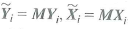
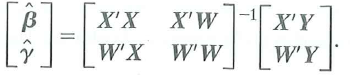
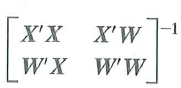
Consider the regression model in matrix form
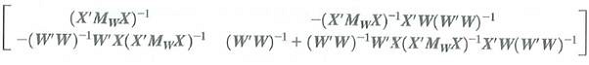
 where X and W are matrices of regressors and ß and are vectors of unknown regression coefficients. Let
 where
where
a. Show that the OLS estimators of ß and can be written as
b. Show that
 =
=
c. Show that
d. The Frisch-Waugh theorem (Appendix 6.2) says that
 Use the result in (c) to prove the Frisch-Waugh theorem.
where X and W are matrices of regressors and ß and are vectors of unknown regression coefficients. Let where a. Show that the OLS estimators of ß and can be written as
b. Show that
= c. Show that
d. The Frisch-Waugh theorem (Appendix 6.2) says that
Use the result in (c) to prove the Frisch-Waugh theorem. Question
Consider the regression model from Chapter 4,
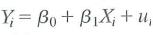 , and assume that the assumptions in Key Concept 4.3 hold.
a. Write the model in the matrix form given in Equations (18.2) and (18.4).
b. Show that Assumptions #1 through #4 in Key Concept 18.1 are satisfied.
c. Use the general formula for
 in Equation (18.11) to derive the expressions for
 and
and
 given in Key Concept 4.2.
d. Show that the (1,1) element of
 in Equation (18.13) is equal to the expression for
 given in Key Concept 4.4.
, and assume that the assumptions in Key Concept 4.3 hold.a. Write the model in the matrix form given in Equations (18.2) and (18.4).
b. Show that Assumptions #1 through #4 in Key Concept 18.1 are satisfied.
c. Use the general formula for
in Equation (18.11) to derive the expressions for and given in Key Concept 4.2.d. Show that the (1,1) element of
in Equation (18.13) is equal to the expression for given in Key Concept 4.4. Question
Question
Question
Construct an example of a regression model that satisfies the assumption
 but for which
but for which Question
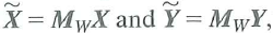
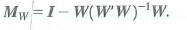
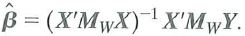
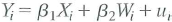
Consider the regression model in matrix form, Y = X + W + U , where X is an n × k 1 matrix of regressors and W is an n × k 2 matrix of regressors. Then, as shown in Exercise 18.17, the OLS estimator ß can be expressed
![Consider the regression model in matrix form, Y = X + W + U , where X is an n × k 1 matrix of regressors and W is an n × k 2 matrix of regressors. Then, as shown in Exercise 18.17, the OLS estimator ß can be expressed Now let be the binary variable fixed effects estimator computed by estimating Equation (10.11) by OLS and let be the de-meaning fixed effects estimator computed by estimating Equation (10.14) by OLS, in which the entity-specific sample means have been subtracted from X and Y. Use the expression for given above to prove that . [ Hint : Write Equation (10.11) using a full set of fixed effects, D 1 i , D 2 i , …, Dn i and no constant term. Include all of the fixed effects in W. Write out the matrix M W X.]<div style=padding-top: 35px>](https://d2lvgg3v3hfg70.cloudfront.net/SM2685/11eb817c_7816_f40b_84e6_f332daa20235_SM2685_11.jpg)
Now let
![Consider the regression model in matrix form, Y = X + W + U , where X is an n × k 1 matrix of regressors and W is an n × k 2 matrix of regressors. Then, as shown in Exercise 18.17, the OLS estimator ß can be expressed Now let be the binary variable fixed effects estimator computed by estimating Equation (10.11) by OLS and let be the de-meaning fixed effects estimator computed by estimating Equation (10.14) by OLS, in which the entity-specific sample means have been subtracted from X and Y. Use the expression for given above to prove that . [ Hint : Write Equation (10.11) using a full set of fixed effects, D 1 i , D 2 i , …, Dn i and no constant term. Include all of the fixed effects in W. Write out the matrix M W X.]<div style=padding-top: 35px>](https://d2lvgg3v3hfg70.cloudfront.net/SM2685/11eb817c_7817_1b1c_84e6_6b7d95a38b28_SM2685_11.jpg) be the "binary variable" fixed effects estimator computed by estimating Equation (10.11) by OLS and let
be the "binary variable" fixed effects estimator computed by estimating Equation (10.11) by OLS and let
![Consider the regression model in matrix form, Y = X + W + U , where X is an n × k 1 matrix of regressors and W is an n × k 2 matrix of regressors. Then, as shown in Exercise 18.17, the OLS estimator ß can be expressed Now let be the binary variable fixed effects estimator computed by estimating Equation (10.11) by OLS and let be the de-meaning fixed effects estimator computed by estimating Equation (10.14) by OLS, in which the entity-specific sample means have been subtracted from X and Y. Use the expression for given above to prove that . [ Hint : Write Equation (10.11) using a full set of fixed effects, D 1 i , D 2 i , …, Dn i and no constant term. Include all of the fixed effects in W. Write out the matrix M W X.]<div style=padding-top: 35px>](https://d2lvgg3v3hfg70.cloudfront.net/SM2685/11eb817c_7817_1b1d_84e6_5922ae13c395_SM2685_11.jpg) be the "de-meaning" fixed effects estimator computed by estimating Equation (10.14) by OLS, in which the entity-specific sample means have been subtracted from X and Y. Use the expression for
be the "de-meaning" fixed effects estimator computed by estimating Equation (10.14) by OLS, in which the entity-specific sample means have been subtracted from X and Y. Use the expression for
![Consider the regression model in matrix form, Y = X + W + U , where X is an n × k 1 matrix of regressors and W is an n × k 2 matrix of regressors. Then, as shown in Exercise 18.17, the OLS estimator ß can be expressed Now let be the binary variable fixed effects estimator computed by estimating Equation (10.11) by OLS and let be the de-meaning fixed effects estimator computed by estimating Equation (10.14) by OLS, in which the entity-specific sample means have been subtracted from X and Y. Use the expression for given above to prove that . [ Hint : Write Equation (10.11) using a full set of fixed effects, D 1 i , D 2 i , …, Dn i and no constant term. Include all of the fixed effects in W. Write out the matrix M W X.]<div style=padding-top: 35px>](https://d2lvgg3v3hfg70.cloudfront.net/SM2685/11eb817c_7817_1b1e_84e6_c387499b93be_SM2685_11.jpg) given above to prove that
given above to prove that
![Consider the regression model in matrix form, Y = X + W + U , where X is an n × k 1 matrix of regressors and W is an n × k 2 matrix of regressors. Then, as shown in Exercise 18.17, the OLS estimator ß can be expressed Now let be the binary variable fixed effects estimator computed by estimating Equation (10.11) by OLS and let be the de-meaning fixed effects estimator computed by estimating Equation (10.14) by OLS, in which the entity-specific sample means have been subtracted from X and Y. Use the expression for given above to prove that . [ Hint : Write Equation (10.11) using a full set of fixed effects, D 1 i , D 2 i , …, Dn i and no constant term. Include all of the fixed effects in W. Write out the matrix M W X.]<div style=padding-top: 35px>](https://d2lvgg3v3hfg70.cloudfront.net/SM2685/11eb817c_7817_1b1f_84e6_c3ba01f39b66_SM2685_11.jpg) . [ Hint : Write Equation (10.11) using a full set of fixed effects, D 1 i , D 2 i , …, Dn i and no constant term. Include all of the fixed effects in W. Write out the matrix M W X.]
. [ Hint : Write Equation (10.11) using a full set of fixed effects, D 1 i , D 2 i , …, Dn i and no constant term. Include all of the fixed effects in W. Write out the matrix M W X.]
Now let
be the "binary variable" fixed effects estimator computed by estimating Equation (10.11) by OLS and let be the "de-meaning" fixed effects estimator computed by estimating Equation (10.14) by OLS, in which the entity-specific sample means have been subtracted from X and Y. Use the expression for given above to prove that . [ Hint : Write Equation (10.11) using a full set of fixed effects, D 1 i , D 2 i , …, Dn i and no constant term. Include all of the fixed effects in W. Write out the matrix M W X.] Question
Consider the regression model,
 where for simplicity the intercept is omitted and all variables are assumed to have a mean of zero. Suppose that Xi is distributed independently of ( w i, u i) but Wi, and ui, might be correlated and let
 and
and
 be the OLS estimators for this model. Show that
a. Whether or not wi, and ui are correlated,

b. If Wi and u i are correlated, then
 is inconsistent.
c. Let
 be the OLS estimator from the regression of Y on X (the restricted regression that excludes IT). Provide conditions under which
 has a smaller asymptotic variance than
 , allowing for the possibility thatWi, and u i are correlated.
where for simplicity the intercept is omitted and all variables are assumed to have a mean of zero. Suppose that Xi is distributed independently of ( w i, u i) but Wi, and ui, might be correlated and let and be the OLS estimators for this model. Show thata. Whether or not wi, and ui are correlated,
b. If Wi and u i are correlated, then
is inconsistent.c. Let
be the OLS estimator from the regression of Y on X (the restricted regression that excludes IT). Provide conditions under which has a smaller asymptotic variance than , allowing for the possibility thatWi, and u i are correlated. Question
Consider the regression model
 where
where
 and u i =
 Suppose that
 , are i.i.d. with mean 0 and variance 1 and are distributed independently of X j : for all i and j.
a. Derive an expression for
b. Explain how to estimate the model by GLS without explicitly inverting the matrix . ( Hint : Transform the model so that the regression errors are
 )
)
where and u i = Suppose that , are i.i.d. with mean 0 and variance 1 and are distributed independently of X j : for all i and j. a. Derive an expression for
b. Explain how to estimate the model by GLS without explicitly inverting the matrix . ( Hint : Transform the model so that the regression errors are
) Question
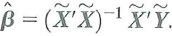
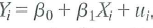
This exercise shows that the OLS estimator of a subset of the regression coefficients is consistent under the conditional mean independence assumption stated in Appendix 7.2. Consider the multiple regression model in matrix form Y=Xß + Wy + u, where X and W are, respectively, n × k 1 and n × k 2 matrices of regressors. Let X i and W i denote the i th rows of X and W [as in Equation (18.3)]. Assume that (i)
![This exercise shows that the OLS estimator of a subset of the regression coefficients is consistent under the conditional mean independence assumption stated in Appendix 7.2. Consider the multiple regression model in matrix form Y=Xß + Wy + u, where X and W are, respectively, n × k 1 and n × k 2 matrices of regressors. Let X i and W i denote the i th rows of X and W [as in Equation (18.3)]. Assume that (i) , where is a k 2 × 1 vector of unknown parameters; (ii) (Xi, W i Yi) are i.i.d.; (iii) (X i W i u i ) have four finite, nonzero moments; and (iv) there is no perfect multicollinearity. These are Assumptions #l-#4 of Key Concept 18.1, with the conditional mean independence assumption (i) replacing the usual conditional mean zero assumption. a. Use the expression for given in Exercise 18.6 to write - ß = . b. Show that where = , and so forth. [The matrix if : for all i,j, where A n,ij and A ij are the (i, j) elements of A n and A.] c. Show that assumptions (i) and (ii) imply that . d. Use (c) and the law of iterated expectations to show that e. Use (a) through (d) to conclude that, under conditions (i) through (iv) <div style=padding-top: 35px>](https://d2lvgg3v3hfg70.cloudfront.net/SM2685/11eb817c_7819_1738_84e6_d3c255040ba1_SM2685_00.jpg) , where is a k 2 × 1 vector of unknown parameters; (ii) (Xi, W i Yi) are i.i.d.; (iii) (X i W i u i ) have four finite, nonzero moments; and (iv) there is no perfect multicollinearity. These are Assumptions #l-#4 of Key Concept 18.1, with the conditional mean independence assumption (i) replacing the usual conditional mean zero assumption.
, where is a k 2 × 1 vector of unknown parameters; (ii) (Xi, W i Yi) are i.i.d.; (iii) (X i W i u i ) have four finite, nonzero moments; and (iv) there is no perfect multicollinearity. These are Assumptions #l-#4 of Key Concept 18.1, with the conditional mean independence assumption (i) replacing the usual conditional mean zero assumption.
a. Use the expression for
![This exercise shows that the OLS estimator of a subset of the regression coefficients is consistent under the conditional mean independence assumption stated in Appendix 7.2. Consider the multiple regression model in matrix form Y=Xß + Wy + u, where X and W are, respectively, n × k 1 and n × k 2 matrices of regressors. Let X i and W i denote the i th rows of X and W [as in Equation (18.3)]. Assume that (i) , where is a k 2 × 1 vector of unknown parameters; (ii) (Xi, W i Yi) are i.i.d.; (iii) (X i W i u i ) have four finite, nonzero moments; and (iv) there is no perfect multicollinearity. These are Assumptions #l-#4 of Key Concept 18.1, with the conditional mean independence assumption (i) replacing the usual conditional mean zero assumption. a. Use the expression for given in Exercise 18.6 to write - ß = . b. Show that where = , and so forth. [The matrix if : for all i,j, where A n,ij and A ij are the (i, j) elements of A n and A.] c. Show that assumptions (i) and (ii) imply that . d. Use (c) and the law of iterated expectations to show that e. Use (a) through (d) to conclude that, under conditions (i) through (iv) <div style=padding-top: 35px>](https://d2lvgg3v3hfg70.cloudfront.net/SM2685/11eb817c_7819_1739_84e6_89ed44a40078_SM2685_11.jpg) given in Exercise 18.6 to write
given in Exercise 18.6 to write
![This exercise shows that the OLS estimator of a subset of the regression coefficients is consistent under the conditional mean independence assumption stated in Appendix 7.2. Consider the multiple regression model in matrix form Y=Xß + Wy + u, where X and W are, respectively, n × k 1 and n × k 2 matrices of regressors. Let X i and W i denote the i th rows of X and W [as in Equation (18.3)]. Assume that (i) , where is a k 2 × 1 vector of unknown parameters; (ii) (Xi, W i Yi) are i.i.d.; (iii) (X i W i u i ) have four finite, nonzero moments; and (iv) there is no perfect multicollinearity. These are Assumptions #l-#4 of Key Concept 18.1, with the conditional mean independence assumption (i) replacing the usual conditional mean zero assumption. a. Use the expression for given in Exercise 18.6 to write - ß = . b. Show that where = , and so forth. [The matrix if : for all i,j, where A n,ij and A ij are the (i, j) elements of A n and A.] c. Show that assumptions (i) and (ii) imply that . d. Use (c) and the law of iterated expectations to show that e. Use (a) through (d) to conclude that, under conditions (i) through (iv) <div style=padding-top: 35px>](https://d2lvgg3v3hfg70.cloudfront.net/SM2685/11eb817c_7819_173a_84e6_83b521b6d389_SM2685_11.jpg) - ß =
- ß =
![This exercise shows that the OLS estimator of a subset of the regression coefficients is consistent under the conditional mean independence assumption stated in Appendix 7.2. Consider the multiple regression model in matrix form Y=Xß + Wy + u, where X and W are, respectively, n × k 1 and n × k 2 matrices of regressors. Let X i and W i denote the i th rows of X and W [as in Equation (18.3)]. Assume that (i) , where is a k 2 × 1 vector of unknown parameters; (ii) (Xi, W i Yi) are i.i.d.; (iii) (X i W i u i ) have four finite, nonzero moments; and (iv) there is no perfect multicollinearity. These are Assumptions #l-#4 of Key Concept 18.1, with the conditional mean independence assumption (i) replacing the usual conditional mean zero assumption. a. Use the expression for given in Exercise 18.6 to write - ß = . b. Show that where = , and so forth. [The matrix if : for all i,j, where A n,ij and A ij are the (i, j) elements of A n and A.] c. Show that assumptions (i) and (ii) imply that . d. Use (c) and the law of iterated expectations to show that e. Use (a) through (d) to conclude that, under conditions (i) through (iv) <div style=padding-top: 35px>](https://d2lvgg3v3hfg70.cloudfront.net/SM2685/11eb817c_7819_173b_84e6_a1cedb886846_SM2685_00.jpg) .
.
b. Show that
![This exercise shows that the OLS estimator of a subset of the regression coefficients is consistent under the conditional mean independence assumption stated in Appendix 7.2. Consider the multiple regression model in matrix form Y=Xß + Wy + u, where X and W are, respectively, n × k 1 and n × k 2 matrices of regressors. Let X i and W i denote the i th rows of X and W [as in Equation (18.3)]. Assume that (i) , where is a k 2 × 1 vector of unknown parameters; (ii) (Xi, W i Yi) are i.i.d.; (iii) (X i W i u i ) have four finite, nonzero moments; and (iv) there is no perfect multicollinearity. These are Assumptions #l-#4 of Key Concept 18.1, with the conditional mean independence assumption (i) replacing the usual conditional mean zero assumption. a. Use the expression for given in Exercise 18.6 to write - ß = . b. Show that where = , and so forth. [The matrix if : for all i,j, where A n,ij and A ij are the (i, j) elements of A n and A.] c. Show that assumptions (i) and (ii) imply that . d. Use (c) and the law of iterated expectations to show that e. Use (a) through (d) to conclude that, under conditions (i) through (iv) <div style=padding-top: 35px>](https://d2lvgg3v3hfg70.cloudfront.net/SM2685/11eb817c_7819_3e4c_84e6_419fc50b4928_SM2685_11.jpg) where
where
![This exercise shows that the OLS estimator of a subset of the regression coefficients is consistent under the conditional mean independence assumption stated in Appendix 7.2. Consider the multiple regression model in matrix form Y=Xß + Wy + u, where X and W are, respectively, n × k 1 and n × k 2 matrices of regressors. Let X i and W i denote the i th rows of X and W [as in Equation (18.3)]. Assume that (i) , where is a k 2 × 1 vector of unknown parameters; (ii) (Xi, W i Yi) are i.i.d.; (iii) (X i W i u i ) have four finite, nonzero moments; and (iv) there is no perfect multicollinearity. These are Assumptions #l-#4 of Key Concept 18.1, with the conditional mean independence assumption (i) replacing the usual conditional mean zero assumption. a. Use the expression for given in Exercise 18.6 to write - ß = . b. Show that where = , and so forth. [The matrix if : for all i,j, where A n,ij and A ij are the (i, j) elements of A n and A.] c. Show that assumptions (i) and (ii) imply that . d. Use (c) and the law of iterated expectations to show that e. Use (a) through (d) to conclude that, under conditions (i) through (iv) <div style=padding-top: 35px>](https://d2lvgg3v3hfg70.cloudfront.net/SM2685/11eb817c_7819_3e4d_84e6_efcf5124c30e_SM2685_11.jpg) =
=
![This exercise shows that the OLS estimator of a subset of the regression coefficients is consistent under the conditional mean independence assumption stated in Appendix 7.2. Consider the multiple regression model in matrix form Y=Xß + Wy + u, where X and W are, respectively, n × k 1 and n × k 2 matrices of regressors. Let X i and W i denote the i th rows of X and W [as in Equation (18.3)]. Assume that (i) , where is a k 2 × 1 vector of unknown parameters; (ii) (Xi, W i Yi) are i.i.d.; (iii) (X i W i u i ) have four finite, nonzero moments; and (iv) there is no perfect multicollinearity. These are Assumptions #l-#4 of Key Concept 18.1, with the conditional mean independence assumption (i) replacing the usual conditional mean zero assumption. a. Use the expression for given in Exercise 18.6 to write - ß = . b. Show that where = , and so forth. [The matrix if : for all i,j, where A n,ij and A ij are the (i, j) elements of A n and A.] c. Show that assumptions (i) and (ii) imply that . d. Use (c) and the law of iterated expectations to show that e. Use (a) through (d) to conclude that, under conditions (i) through (iv) <div style=padding-top: 35px>](https://d2lvgg3v3hfg70.cloudfront.net/SM2685/11eb817c_7819_3e4e_84e6_2747feb4e91c_SM2685_11.jpg) , and so forth. [The matrix
, and so forth. [The matrix
![This exercise shows that the OLS estimator of a subset of the regression coefficients is consistent under the conditional mean independence assumption stated in Appendix 7.2. Consider the multiple regression model in matrix form Y=Xß + Wy + u, where X and W are, respectively, n × k 1 and n × k 2 matrices of regressors. Let X i and W i denote the i th rows of X and W [as in Equation (18.3)]. Assume that (i) , where is a k 2 × 1 vector of unknown parameters; (ii) (Xi, W i Yi) are i.i.d.; (iii) (X i W i u i ) have four finite, nonzero moments; and (iv) there is no perfect multicollinearity. These are Assumptions #l-#4 of Key Concept 18.1, with the conditional mean independence assumption (i) replacing the usual conditional mean zero assumption. a. Use the expression for given in Exercise 18.6 to write - ß = . b. Show that where = , and so forth. [The matrix if : for all i,j, where A n,ij and A ij are the (i, j) elements of A n and A.] c. Show that assumptions (i) and (ii) imply that . d. Use (c) and the law of iterated expectations to show that e. Use (a) through (d) to conclude that, under conditions (i) through (iv) <div style=padding-top: 35px>](https://d2lvgg3v3hfg70.cloudfront.net/SM2685/11eb817c_7819_3e4f_84e6_33abc4666f19_SM2685_11.jpg) if
if
![This exercise shows that the OLS estimator of a subset of the regression coefficients is consistent under the conditional mean independence assumption stated in Appendix 7.2. Consider the multiple regression model in matrix form Y=Xß + Wy + u, where X and W are, respectively, n × k 1 and n × k 2 matrices of regressors. Let X i and W i denote the i th rows of X and W [as in Equation (18.3)]. Assume that (i) , where is a k 2 × 1 vector of unknown parameters; (ii) (Xi, W i Yi) are i.i.d.; (iii) (X i W i u i ) have four finite, nonzero moments; and (iv) there is no perfect multicollinearity. These are Assumptions #l-#4 of Key Concept 18.1, with the conditional mean independence assumption (i) replacing the usual conditional mean zero assumption. a. Use the expression for given in Exercise 18.6 to write - ß = . b. Show that where = , and so forth. [The matrix if : for all i,j, where A n,ij and A ij are the (i, j) elements of A n and A.] c. Show that assumptions (i) and (ii) imply that . d. Use (c) and the law of iterated expectations to show that e. Use (a) through (d) to conclude that, under conditions (i) through (iv) <div style=padding-top: 35px>](https://d2lvgg3v3hfg70.cloudfront.net/SM2685/11eb817c_7819_3e50_84e6_e3428034e6e6_SM2685_11.jpg) : for all i,j, where A n,ij and A ij are the (i, j) elements of A n and A.]
: for all i,j, where A n,ij and A ij are the (i, j) elements of A n and A.]
c. Show that assumptions (i) and (ii) imply that
![This exercise shows that the OLS estimator of a subset of the regression coefficients is consistent under the conditional mean independence assumption stated in Appendix 7.2. Consider the multiple regression model in matrix form Y=Xß + Wy + u, where X and W are, respectively, n × k 1 and n × k 2 matrices of regressors. Let X i and W i denote the i th rows of X and W [as in Equation (18.3)]. Assume that (i) , where is a k 2 × 1 vector of unknown parameters; (ii) (Xi, W i Yi) are i.i.d.; (iii) (X i W i u i ) have four finite, nonzero moments; and (iv) there is no perfect multicollinearity. These are Assumptions #l-#4 of Key Concept 18.1, with the conditional mean independence assumption (i) replacing the usual conditional mean zero assumption. a. Use the expression for given in Exercise 18.6 to write - ß = . b. Show that where = , and so forth. [The matrix if : for all i,j, where A n,ij and A ij are the (i, j) elements of A n and A.] c. Show that assumptions (i) and (ii) imply that . d. Use (c) and the law of iterated expectations to show that e. Use (a) through (d) to conclude that, under conditions (i) through (iv) <div style=padding-top: 35px>](https://d2lvgg3v3hfg70.cloudfront.net/SM2685/11eb817c_7819_3e51_84e6_7d0cbc58dfde_SM2685_11.jpg) .
.
d. Use (c) and the law of iterated expectations to show that
![This exercise shows that the OLS estimator of a subset of the regression coefficients is consistent under the conditional mean independence assumption stated in Appendix 7.2. Consider the multiple regression model in matrix form Y=Xß + Wy + u, where X and W are, respectively, n × k 1 and n × k 2 matrices of regressors. Let X i and W i denote the i th rows of X and W [as in Equation (18.3)]. Assume that (i) , where is a k 2 × 1 vector of unknown parameters; (ii) (Xi, W i Yi) are i.i.d.; (iii) (X i W i u i ) have four finite, nonzero moments; and (iv) there is no perfect multicollinearity. These are Assumptions #l-#4 of Key Concept 18.1, with the conditional mean independence assumption (i) replacing the usual conditional mean zero assumption. a. Use the expression for given in Exercise 18.6 to write - ß = . b. Show that where = , and so forth. [The matrix if : for all i,j, where A n,ij and A ij are the (i, j) elements of A n and A.] c. Show that assumptions (i) and (ii) imply that . d. Use (c) and the law of iterated expectations to show that e. Use (a) through (d) to conclude that, under conditions (i) through (iv) <div style=padding-top: 35px>](https://d2lvgg3v3hfg70.cloudfront.net/SM2685/11eb817c_7819_3e52_84e6_3f2d040e0736_SM2685_11.jpg)
e. Use (a) through (d) to conclude that, under conditions (i) through
(iv)
![This exercise shows that the OLS estimator of a subset of the regression coefficients is consistent under the conditional mean independence assumption stated in Appendix 7.2. Consider the multiple regression model in matrix form Y=Xß + Wy + u, where X and W are, respectively, n × k 1 and n × k 2 matrices of regressors. Let X i and W i denote the i th rows of X and W [as in Equation (18.3)]. Assume that (i) , where is a k 2 × 1 vector of unknown parameters; (ii) (Xi, W i Yi) are i.i.d.; (iii) (X i W i u i ) have four finite, nonzero moments; and (iv) there is no perfect multicollinearity. These are Assumptions #l-#4 of Key Concept 18.1, with the conditional mean independence assumption (i) replacing the usual conditional mean zero assumption. a. Use the expression for given in Exercise 18.6 to write - ß = . b. Show that where = , and so forth. [The matrix if : for all i,j, where A n,ij and A ij are the (i, j) elements of A n and A.] c. Show that assumptions (i) and (ii) imply that . d. Use (c) and the law of iterated expectations to show that e. Use (a) through (d) to conclude that, under conditions (i) through (iv) <div style=padding-top: 35px>](https://d2lvgg3v3hfg70.cloudfront.net/SM2685/11eb817c_7819_3e53_84e6_912728cdc5a9_SM2685_11.jpg)
, where is a k 2 × 1 vector of unknown parameters; (ii) (Xi, W i Yi) are i.i.d.; (iii) (X i W i u i ) have four finite, nonzero moments; and (iv) there is no perfect multicollinearity. These are Assumptions #l-#4 of Key Concept 18.1, with the conditional mean independence assumption (i) replacing the usual conditional mean zero assumption.a. Use the expression for
given in Exercise 18.6 to write - ß = . b. Show that
where = , and so forth. [The matrix if : for all i,j, where A n,ij and A ij are the (i, j) elements of A n and A.] c. Show that assumptions (i) and (ii) imply that
.d. Use (c) and the law of iterated expectations to show that
e. Use (a) through (d) to conclude that, under conditions (i) through
(iv)
Question

Unlock Deck
Sign up to unlock the cards in this deck!
Unlock Deck
Unlock Deck
1/22
Play
Full screen (f)
Deck 18: The Theory of Multiple Regression
1
Suppose that C is an n × n symmetric idempotent matrix with rank r and let V ~ N (0 n , I n ).
a. Show that C = AA ', where A is n × r with A'A = I r. ( Hint: C is possintive semidefinite and can be written as Q Q as explained in Appendix 18.1.)
b. Show that A'V ~ N ( 0 r , I r ).
c. Show that V'CV ~ r 2
a. Show that C = AA ', where A is n × r with A'A = I r. ( Hint: C is possintive semidefinite and can be written as Q Q as explained in Appendix 18.1.)
b. Show that A'V ~ N ( 0 r , I r ).
c. Show that V'CV ~ r 2
a) Since C is semidefinite and positive
 The matrix form is

 Hence for some matrix A
 The matrix will be
 b) Since V ~ N ( 0 n , I n ) then its multiple with the matrix A will be distributed
 c) The given equation is
 Since A ' V is normally distributed with mean 0 and variance I the term
 contains sums of the matrices will be distributed Chi-squared.
The matrix form is Hence for some matrix A The matrix will be b) Since V ~ N ( 0 n , I n ) then its multiple with the matrix A will be distributed c) The given equation is Since A ' V is normally distributed with mean 0 and variance I the term contains sums of the matrices will be distributed Chi-squared. 2
Consider the population regression of test scores against income and the square of income in Equation (8.1).
a. Write the regression in Equation (8.1) in the matrix form of Equation (18.5). Define Y,X,U, and ß.
b. Explain how to test the null hypothesis that the relationship between test scores and income is linear against the alternative that it is quadratic. Write the null hypothesis in the form of Equation (18.20). What are R, r, and q
a) Let the following be the general linear regression
 Here the variables are matrices, Y corresponds to the dependent variable test scores, X corresponds to the independent variable matrix which stores the coefficient column, income and squared income, ß stores the regression coefficients, and U is the error vector as defined below
 As seen from the equation there are n observations for each dependent and independent variable.
b) The test for the hypothesis have the form
 To test for a linear against a quadratic, the null is
 The (0 0 1) stores the test information in R. For example, multiplying the matrices gives
 Which is the hypothesis the it is not quadratic, hence linear. There is only one restriction so q = 1.
Here the variables are matrices, Y corresponds to the dependent variable test scores, X corresponds to the independent variable matrix which stores the coefficient column, income and squared income, ß stores the regression coefficients, and U is the error vector as defined below As seen from the equation there are n observations for each dependent and independent variable. b) The test for the hypothesis have the form
To test for a linear against a quadratic, the null is The (0 0 1) stores the test information in R. For example, multiplying the matrices gives Which is the hypothesis the it is not quadratic, hence linear. There is only one restriction so q = 1. 3
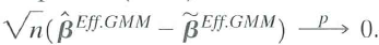
Show that
is the efficient GMM estimator-that is, that
Equation (18.66) is the solution to Equation (18.65).
b. Show that
c. Show that
is the efficient GMM estimator-that is, that Equation (18.66) is the solution to Equation (18.65).b. Show that
c. Show that
a) The following matrix is to be minimized by b
 Taking the derivative with respect to b
 This is the definition of the GMM estimator.
b) Both estimators
 converges to
 hence
hence
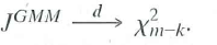
 c) The J stat is a multiple of matrices with normal distribution hence it will follow a chi-squared distribution.
Taking the derivative with respect to b This is the definition of the GMM estimator. b) Both estimators
converges to hence c) The J stat is a multiple of matrices with normal distribution hence it will follow a chi-squared distribution. 4
A researcher studying the relationship between earnings and gender for a group of workers specifies the regression model, Y i = ß 0 + X 1 i ß 1 + X 2 i ß 2 + u i , where X 1 i is a binary variable that equals 1 if the i th person is a female and X 2i is a binary variable that equals 1 if the i th person is a male. Write the model in the matrix form of Equation (18.2) for a hypothetical set of n = 5 observations. Show that the columns of X are linearly dependent so that X does not have full rank. Explain how you would respecifiy the model to eliminate the perfect multicollinearity.
Unlock Deck
Unlock for access to all 22 flashcards in this deck.
Unlock Deck
k this deck
5
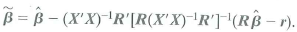
Consider the problem of minimizing the sum of squared residuals subject to the constraint that Rb = r, where R is q × ( k + 1) with rank cj. Let
be the value of b that solves the constrained minimization problem.
a. Show that the Lagrangian for the minimization problem is L(b , ) = ( Y- Xb ) ' ( Y-Xb ) + ' ( Rb - r ), where is a q × 1 vector of Lagrange multipliers.
b. Show that
c. Show that
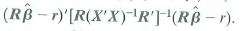
d. Show that F in Equation (18.36) is equivalent to the homoskeskasticity-only F -statistic in Equation (7.13).
be the value of b that solves the constrained minimization problem.a. Show that the Lagrangian for the minimization problem is L(b , ) = ( Y- Xb ) ' ( Y-Xb ) + ' ( Rb - r ), where is a q × 1 vector of Lagrange multipliers.
b. Show that
c. Show that
d. Show that F in Equation (18.36) is equivalent to the homoskeskasticity-only F -statistic in Equation (7.13).
Unlock Deck
Unlock for access to all 22 flashcards in this deck.
Unlock Deck
k this deck
6
Suppose that a sample of n = 20 households has the sample means and sample covariances below for a dependent variable and two regressors:
a. Calculate the OLS estimates of ß 0 , ß h and ß 2 Calculate s 2 u ,. Calculate the R 2 of the regression.
b. Suppose that all six assumptions in Key Concept 18.1 hold. Test the hypothesis that ß 1 = 0 at the 5% significance level.
a. Calculate the OLS estimates of ß 0 , ß h and ß 2 Calculate s 2 u ,. Calculate the R 2 of the regression.b. Suppose that all six assumptions in Key Concept 18.1 hold. Test the hypothesis that ß 1 = 0 at the 5% significance level.
Unlock Deck
Unlock for access to all 22 flashcards in this deck.
Unlock Deck
k this deck
7
Consider the regression model Y = Xß + U. Partition X as [ X 1 X 2 ] and ß as
where X 1 has k 1 columns and X 2 has k 2 columns. Suppose that
Let
a. Show that
b. Consider the regression described in Equation (12.17). Let W = [1 W 1 W 2 … W r ], where 1 is an n × 1 vector of ones, W l is the n X 1 vector with i th element W 1 i and so forth. Let
denote the vector of two stage least squares residuals.
i. Show that
ii. Show that the method for computing the J -statistic described in Key Concept 12.6 (using a homoskedasiticity-only F-statistic) and the formula in Equation (18.63) produce the same value for the J -statistic. [Hint: Use the results in (a), (b, i), and Exercise 18.13.]
where X 1 has k 1 columns and X 2 has k 2 columns. Suppose that Let a. Show that
b. Consider the regression described in Equation (12.17). Let W = [1 W 1 W 2 … W r ], where 1 is an n × 1 vector of ones, W l is the n X 1 vector with i th element W 1 i and so forth. Let
denote the vector of two stage least squares residuals.i. Show that
ii. Show that the method for computing the J -statistic described in Key Concept 12.6 (using a homoskedasiticity-only F-statistic) and the formula in Equation (18.63) produce the same value for the J -statistic. [Hint: Use the results in (a), (b, i), and Exercise 18.13.]
Unlock Deck
Unlock for access to all 22 flashcards in this deck.
Unlock Deck
k this deck
8
You are analyzing a linear regression model with 500 observations and one regressor. Explain how you would construct a confidence interval for ß 1 if:
a. Assumptions #1 through #4 in Key Concept 18.1 are true, but you think Assumption #5 or #6 might not be true.
b. Assumptions #1 through #5 are true, but you think Assumption #6 might not be true.(give two ways to construct the confidence interval).
c. Assumptions #1 through #6 are true
a. Assumptions #1 through #4 in Key Concept 18.1 are true, but you think Assumption #5 or #6 might not be true.
b. Assumptions #1 through #5 are true, but you think Assumption #6 might not be true.(give two ways to construct the confidence interval).
c. Assumptions #1 through #6 are true
Unlock Deck
Unlock for access to all 22 flashcards in this deck.
Unlock Deck
k this deck
9
(Consistency of clustered standard errors.) Consider the panel data model
where all variables are scalars. Assume that Assumption #1, #2, and #4 in Key Concept 10.3 hold and strengthen Assumption #3 so that X it and u it have eight nonzero finite moments. Let M = I T T 1 , where is a T × 1 vector ones, Also let Y i = ( Y i 1 · Y i 2 … Y iT ) , X i = ( X i 1 X i 2 … X iT ) , u i = ( u i 1 u i 2 … u iT ) ,
, and
. For the asymptotic calculations in this problem, suppose that T is fixed and n
where all variables are scalars. Assume that Assumption #1, #2, and #4 in Key Concept 10.3 hold and strengthen Assumption #3 so that X it and u it have eight nonzero finite moments. Let M = I T T 1 , where is a T × 1 vector ones, Also let Y i = ( Y i 1 · Y i 2 … Y iT ) , X i = ( X i 1 X i 2 … X iT ) , u i = ( u i 1 u i 2 … u iT ) , , and . For the asymptotic calculations in this problem, suppose that T is fixed and n Unlock Deck
Unlock for access to all 22 flashcards in this deck.
Unlock Deck
k this deck
10
Let W be an m × 1 vector with covariance matrix
where
is finite and positive definite. Let c be a nonrandom m × 1 vector, and let
a. Show that var
b. Suppose that c 0 m Show that 0 var(Q) .
where is finite and positive definite. Let c be a nonrandom m × 1 vector, and let a. Show that var
b. Suppose that c 0 m Show that 0 var(Q) .
Unlock Deck
Unlock for access to all 22 flashcards in this deck.
Unlock Deck
k this deck
11
This exercise takes up the problem of missing data discussed in Section 9.2. Consider the regression model
where all variables are scalars and the constant term/intercept is omitted for convenience.
a. Suppose that the least assumptions in Key Concept 4.3 are satisfied. Show that the least squares estimator of ß is unbiased and consistent.
b. Now suppose that some of the observations are missing. Let I i , denote a binary random variable that indicates the nonmissing observations; that is, I i = 1 if observation i is not missing and I i = 0 if observation i is missing. Assume that
are i.i.d.
i. Show that the OLS estimator can be written as
ii. Suppose that data are "missing completely at random" in the sense that
where p is a constant. Show that
is unbiased and consistent.
iii. Suppose that the probability that the i th observation is missing depends of X i but not on u i ; that is,
Show that
is unbiased and consistent.
iv. Suppose that the probability that the i th observation is missing depends on both X i and u i ; that is,
Is
unbiased Is
consistent Explain.
c. Suppose that ß = 1 and that X i and u i are mutually independent standard normal random variables [so that both X t and iq are distributed N (0,1)]. Suppose that I i = 1 when Y i 0, but I i = 0 when Y i 0. Is
unbiased Is
consistent Explain.
where all variables are scalars and the constant term/intercept is omitted for convenience.a. Suppose that the least assumptions in Key Concept 4.3 are satisfied. Show that the least squares estimator of ß is unbiased and consistent.
b. Now suppose that some of the observations are missing. Let I i , denote a binary random variable that indicates the nonmissing observations; that is, I i = 1 if observation i is not missing and I i = 0 if observation i is missing. Assume that
are i.i.d.i. Show that the OLS estimator can be written as
ii. Suppose that data are "missing completely at random" in the sense that
where p is a constant. Show that is unbiased and consistent.iii. Suppose that the probability that the i th observation is missing depends of X i but not on u i ; that is,
Show that is unbiased and consistent.iv. Suppose that the probability that the i th observation is missing depends on both X i and u i ; that is,
Is unbiased Is consistent Explain.c. Suppose that ß = 1 and that X i and u i are mutually independent standard normal random variables [so that both X t and iq are distributed N (0,1)]. Suppose that I i = 1 when Y i 0, but I i = 0 when Y i 0. Is
unbiased Is consistent Explain. Unlock Deck
Unlock for access to all 22 flashcards in this deck.
Unlock Deck
k this deck
12
Suppose that Assumptions #1 through #5 in Key Concept 18.1 are true, but that Assumption #6 is not. Does the result in Equation (18.31) hold Explain.
Unlock Deck
Unlock for access to all 22 flashcards in this deck.
Unlock Deck
k this deck
13
Consider the regression model in matrix form
where X and W are matrices of regressors and ß and are vectors of unknown regression coefficients. Let
where
a. Show that the OLS estimators of ß and can be written as
b. Show that
=
c. Show that
d. The Frisch-Waugh theorem (Appendix 6.2) says that
Use the result in (c) to prove the Frisch-Waugh theorem.
where X and W are matrices of regressors and ß and are vectors of unknown regression coefficients. Let where a. Show that the OLS estimators of ß and can be written as
b. Show that
= c. Show that
d. The Frisch-Waugh theorem (Appendix 6.2) says that
Use the result in (c) to prove the Frisch-Waugh theorem. Unlock Deck
Unlock for access to all 22 flashcards in this deck.
Unlock Deck
k this deck
14
Consider the regression model from Chapter 4,
, and assume that the assumptions in Key Concept 4.3 hold.
a. Write the model in the matrix form given in Equations (18.2) and (18.4).
b. Show that Assumptions #1 through #4 in Key Concept 18.1 are satisfied.
c. Use the general formula for
in Equation (18.11) to derive the expressions for
and
given in Key Concept 4.2.
d. Show that the (1,1) element of
in Equation (18.13) is equal to the expression for
given in Key Concept 4.4.
, and assume that the assumptions in Key Concept 4.3 hold.a. Write the model in the matrix form given in Equations (18.2) and (18.4).
b. Show that Assumptions #1 through #4 in Key Concept 18.1 are satisfied.
c. Use the general formula for
in Equation (18.11) to derive the expressions for and given in Key Concept 4.2.d. Show that the (1,1) element of
in Equation (18.13) is equal to the expression for given in Key Concept 4.4. Unlock Deck
Unlock for access to all 22 flashcards in this deck.
Unlock Deck
k this deck
15
Can you compute the BLUE estimator of if Equation (18.41) holds and you do not know What if you know
Unlock Deck
Unlock for access to all 22 flashcards in this deck.
Unlock Deck
k this deck
16
Let P x and M x be as defined in Equations (18.24) and (18.25).
a. Prove that P X M X = 0 n×n and that P x and M x are idempotent.
b. Derive Equations (18.27) and (18.28).
a. Prove that P X M X = 0 n×n and that P x and M x are idempotent.
b. Derive Equations (18.27) and (18.28).
Unlock Deck
Unlock for access to all 22 flashcards in this deck.
Unlock Deck
k this deck
17
Construct an example of a regression model that satisfies the assumption
but for which
but for which Unlock Deck
Unlock for access to all 22 flashcards in this deck.
Unlock Deck
k this deck
18
Consider the regression model in matrix form, Y = X + W + U , where X is an n × k 1 matrix of regressors and W is an n × k 2 matrix of regressors. Then, as shown in Exercise 18.17, the OLS estimator ß can be expressed
Now let
be the "binary variable" fixed effects estimator computed by estimating Equation (10.11) by OLS and let
be the "de-meaning" fixed effects estimator computed by estimating Equation (10.14) by OLS, in which the entity-specific sample means have been subtracted from X and Y. Use the expression for
given above to prove that
. [ Hint : Write Equation (10.11) using a full set of fixed effects, D 1 i , D 2 i , …, Dn i and no constant term. Include all of the fixed effects in W. Write out the matrix M W X.]
Now let
be the "binary variable" fixed effects estimator computed by estimating Equation (10.11) by OLS and let be the "de-meaning" fixed effects estimator computed by estimating Equation (10.14) by OLS, in which the entity-specific sample means have been subtracted from X and Y. Use the expression for given above to prove that . [ Hint : Write Equation (10.11) using a full set of fixed effects, D 1 i , D 2 i , …, Dn i and no constant term. Include all of the fixed effects in W. Write out the matrix M W X.] Unlock Deck
Unlock for access to all 22 flashcards in this deck.
Unlock Deck
k this deck
19
Consider the regression model,
where for simplicity the intercept is omitted and all variables are assumed to have a mean of zero. Suppose that Xi is distributed independently of ( w i, u i) but Wi, and ui, might be correlated and let
and
be the OLS estimators for this model. Show that
a. Whether or not wi, and ui are correlated,
b. If Wi and u i are correlated, then
is inconsistent.
c. Let
be the OLS estimator from the regression of Y on X (the restricted regression that excludes IT). Provide conditions under which
has a smaller asymptotic variance than
, allowing for the possibility thatWi, and u i are correlated.
where for simplicity the intercept is omitted and all variables are assumed to have a mean of zero. Suppose that Xi is distributed independently of ( w i, u i) but Wi, and ui, might be correlated and let and be the OLS estimators for this model. Show thata. Whether or not wi, and ui are correlated,
b. If Wi and u i are correlated, then
is inconsistent.c. Let
be the OLS estimator from the regression of Y on X (the restricted regression that excludes IT). Provide conditions under which has a smaller asymptotic variance than , allowing for the possibility thatWi, and u i are correlated. Unlock Deck
Unlock for access to all 22 flashcards in this deck.
Unlock Deck
k this deck
20
Consider the regression model
where
and u i =
Suppose that
, are i.i.d. with mean 0 and variance 1 and are distributed independently of X j : for all i and j.
a. Derive an expression for
b. Explain how to estimate the model by GLS without explicitly inverting the matrix . ( Hint : Transform the model so that the regression errors are
)
where and u i = Suppose that , are i.i.d. with mean 0 and variance 1 and are distributed independently of X j : for all i and j. a. Derive an expression for
b. Explain how to estimate the model by GLS without explicitly inverting the matrix . ( Hint : Transform the model so that the regression errors are
) Unlock Deck
Unlock for access to all 22 flashcards in this deck.
Unlock Deck
k this deck
21
This exercise shows that the OLS estimator of a subset of the regression coefficients is consistent under the conditional mean independence assumption stated in Appendix 7.2. Consider the multiple regression model in matrix form Y=Xß + Wy + u, where X and W are, respectively, n × k 1 and n × k 2 matrices of regressors. Let X i and W i denote the i th rows of X and W [as in Equation (18.3)]. Assume that (i)
, where is a k 2 × 1 vector of unknown parameters; (ii) (Xi, W i Yi) are i.i.d.; (iii) (X i W i u i ) have four finite, nonzero moments; and (iv) there is no perfect multicollinearity. These are Assumptions #l-#4 of Key Concept 18.1, with the conditional mean independence assumption (i) replacing the usual conditional mean zero assumption.
a. Use the expression for
given in Exercise 18.6 to write
- ß =
.
b. Show that
where
=
, and so forth. [The matrix
if
: for all i,j, where A n,ij and A ij are the (i, j) elements of A n and A.]
c. Show that assumptions (i) and (ii) imply that
.
d. Use (c) and the law of iterated expectations to show that
e. Use (a) through (d) to conclude that, under conditions (i) through
(iv)
, where is a k 2 × 1 vector of unknown parameters; (ii) (Xi, W i Yi) are i.i.d.; (iii) (X i W i u i ) have four finite, nonzero moments; and (iv) there is no perfect multicollinearity. These are Assumptions #l-#4 of Key Concept 18.1, with the conditional mean independence assumption (i) replacing the usual conditional mean zero assumption.a. Use the expression for
given in Exercise 18.6 to write - ß = . b. Show that
where = , and so forth. [The matrix if : for all i,j, where A n,ij and A ij are the (i, j) elements of A n and A.] c. Show that assumptions (i) and (ii) imply that
.d. Use (c) and the law of iterated expectations to show that
e. Use (a) through (d) to conclude that, under conditions (i) through
(iv)
Unlock Deck
Unlock for access to all 22 flashcards in this deck.
Unlock Deck
k this deck
22
Let C be a symmetric idempotent matrix.
a. Show that the eigenvalues of C are either 0 or 1. ( Hint: Note that Cq = q implies 0 = Cq q = CCq q = CCq q = 2 q q and solve for .)
b. Show that trace( C ) = rank( C ).
c. Let d be a n × 1 vector. Show that d'Cd 0.
a. Show that the eigenvalues of C are either 0 or 1. ( Hint: Note that Cq = q implies 0 = Cq q = CCq q = CCq q = 2 q q and solve for .)
b. Show that trace( C ) = rank( C ).
c. Let d be a n × 1 vector. Show that d'Cd 0.
Unlock Deck
Unlock for access to all 22 flashcards in this deck.
Unlock Deck
k this deck
Unlock Deck
Unlock for access to all 22 flashcards in this deck.


