Deck 16: Within-Subjects Anovas
Full screen (f)
Question
Question
Note: Data files for these exercises are available at the publisher's website for this text, http://www.pearsonhighered.com/stern2e.
As previously described in Exercise 1 , in April, 1992, the minimum wage in New Jersey went from $4.25 to $5.05 an hour. The data in file MinWage.sav was obtained from randomly selected fast food restaurants about one month before and eight months after the minimum wage increase took effect.
1. Determine whether the change in the price of a small fry before ( Pfry1 ) and after ( Pfry2 ) the wage raise differs significantly in New Jersey
2. Perform the analysis posed above for the restaurants in Pennsylvania.
Exercise 1
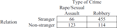
The data below show the number of crime victims as a function of the variables type of crime (rape/sexual assault, robbery) and relation between assailant and victim (stranger, non-stranger). Use the data to determine if the variables are related.
As previously described in Exercise 1 , in April, 1992, the minimum wage in New Jersey went from $4.25 to $5.05 an hour. The data in file MinWage.sav was obtained from randomly selected fast food restaurants about one month before and eight months after the minimum wage increase took effect.
1. Determine whether the change in the price of a small fry before ( Pfry1 ) and after ( Pfry2 ) the wage raise differs significantly in New Jersey
2. Perform the analysis posed above for the restaurants in Pennsylvania.
Exercise 1
The data below show the number of crime victims as a function of the variables type of crime (rape/sexual assault, robbery) and relation between assailant and victim (stranger, non-stranger). Use the data to determine if the variables are related.
Question

Unlock Deck
Sign up to unlock the cards in this deck!
Unlock Deck
Unlock Deck
1/3
Play
Full screen (f)
Deck 16: Within-Subjects Anovas
Note: Data files for these exercises are available at the publisher's website for this text, http://www.pearsonhighered.com/stern2e.
Each year, the Bureau of Transportation Statistics gathers data on various aspects of the U.S. airline industry's performance, including the incidence of mishandled baggage, that is, luggage reported as lost, damaged, delayed, or stolen. The data in file Airline.sav shows the rate of mishandled baggage per 1,000 passengers reported by U.S. airline companies over a three year period from 2004-2006. Use the data in this file to answer the following questions:
1. Has there been a significant change in the mean rate of mishandled baggage over the three-year period
2. Is there a significant linear trend in the mean rate of mishandled baggage over the three-year period
1)
We test to determine whether the significant change in the mean rate of mishandled baggage over the three years period.
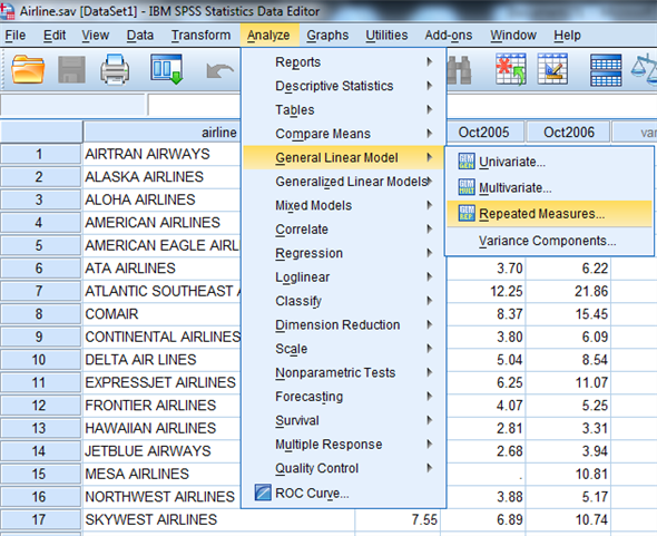
Using SPSS, following is the procedure for obtaining the ANOVA output for the given data.
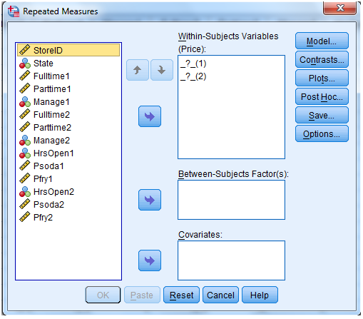
1) Select Analyze, general linear model and repeated measures.
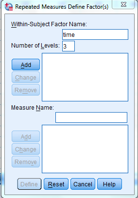
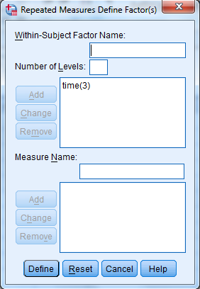
 2) When Repeated measures define Factor(s) dialog box appears type time in within subject factor name and 3 in number of levels. Presss Add button and select define option.
 3) Shift Click to highlight each level name then transfer them by clicking this button.
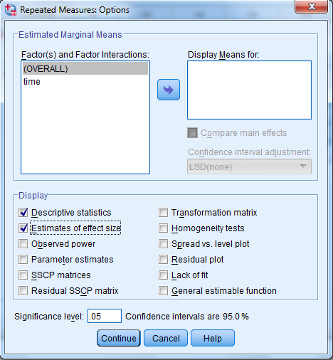
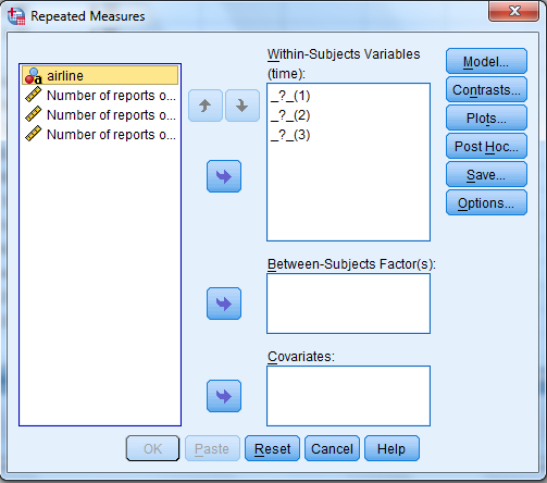 4) Select Options and Continue buttons.
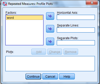
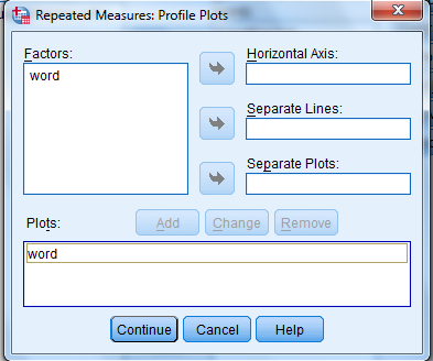
 5) Click Plots button.
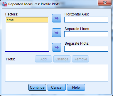 6) Click to highlight the factor name then transfer it to the Horizontal Axis, click Add button and Continue.
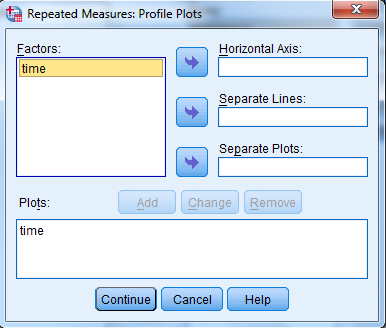 7) Click Ok to run the analysis.
The output is shown below:
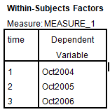
The table below shows the name given to the factor and the number of levels of the factor together with their names.
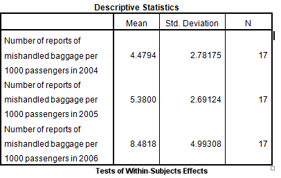
 The table below shows the mean and standard deviation of each time period.
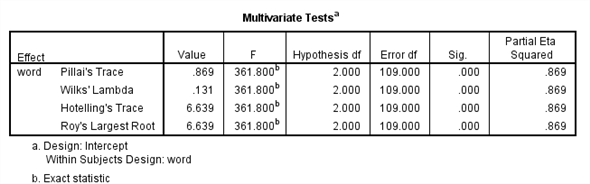
 The table below shows the
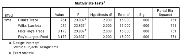
 value and its level of significance for testing the equality of means of the factor.
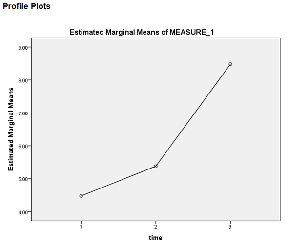 From the output test within subject effect the P -value is 0.000, it is very less, so there is a significant change in the mean rate of mishandled baggage over the three years periods.
2)
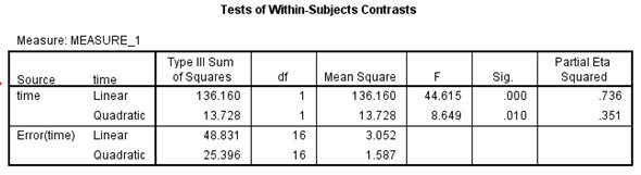
We test to determine whether there is significant linear trend in the mean rate of mishandled baggage over the three years period.
The null and alternative hypotheses are,
 There is no significant linear trend in the mean rate of mishandled baggage over the three years period.
 There is significant linear trend in the mean rate of mishandled baggage over the three years period.
Under the null hypothesis the test statistic is defined as,
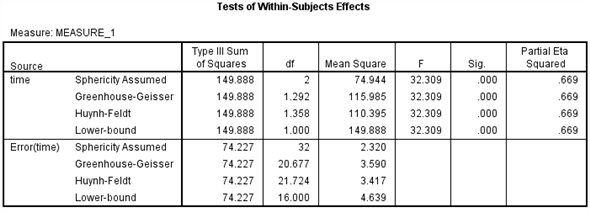
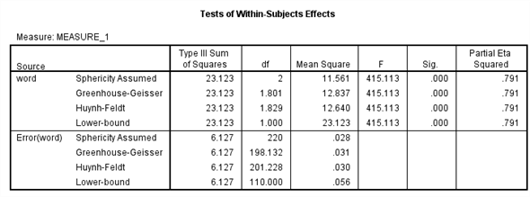
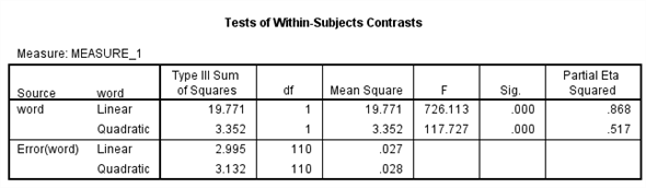
 From the output test of within subjects effects ,
The
 is 44.615
The
 value is 0.000
Here we observe that the
 value is less, so the linear effect of the time is highly significanct.
We test to determine whether the significant change in the mean rate of mishandled baggage over the three years period.
Using SPSS, following is the procedure for obtaining the ANOVA output for the given data.
1) Select Analyze, general linear model and repeated measures.
2) When Repeated measures define Factor(s) dialog box appears type time in within subject factor name and 3 in number of levels. Presss Add button and select define option. 3) Shift Click to highlight each level name then transfer them by clicking this button. 4) Select Options and Continue buttons. 5) Click Plots button. 6) Click to highlight the factor name then transfer it to the Horizontal Axis, click Add button and Continue. 7) Click Ok to run the analysis.The output is shown below:
The table below shows the name given to the factor and the number of levels of the factor together with their names.
The table below shows the mean and standard deviation of each time period. The table below shows the value and its level of significance for testing the equality of means of the factor. From the output test within subject effect the P -value is 0.000, it is very less, so there is a significant change in the mean rate of mishandled baggage over the three years periods.2)
We test to determine whether there is significant linear trend in the mean rate of mishandled baggage over the three years period.
The null and alternative hypotheses are,
There is no significant linear trend in the mean rate of mishandled baggage over the three years period. There is significant linear trend in the mean rate of mishandled baggage over the three years period.Under the null hypothesis the test statistic is defined as,
From the output test of within subjects effects ,The
is 44.615The
value is 0.000Here we observe that the
value is less, so the linear effect of the time is highly significanct.Note: Data files for these exercises are available at the publisher's website for this text, http://www.pearsonhighered.com/stern2e.
As previously described in Exercise 1 , in April, 1992, the minimum wage in New Jersey went from $4.25 to $5.05 an hour. The data in file MinWage.sav was obtained from randomly selected fast food restaurants about one month before and eight months after the minimum wage increase took effect.
1. Determine whether the change in the price of a small fry before ( Pfry1 ) and after ( Pfry2 ) the wage raise differs significantly in New Jersey
2. Perform the analysis posed above for the restaurants in Pennsylvania.
Exercise 1
The data below show the number of crime victims as a function of the variables type of crime (rape/sexual assault, robbery) and relation between assailant and victim (stranger, non-stranger). Use the data to determine if the variables are related.
From the given information in the state variable 0 represents the Pennsylvania.
And 1 represents New Jersey
1)
We test to determine whether the change in price of a small fry before ( Pfry1) and after ( Pfry2) the wage raise differs significantly in New Jersey.
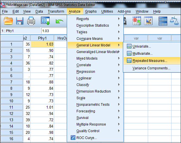
Using SPSS, following is the procedure for obtaining the ANOVA output for the given data.
1) Select Analyze, general linear model and repeated measures.
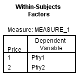
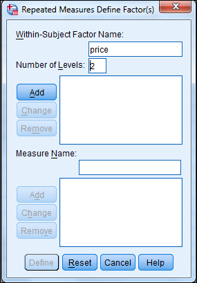
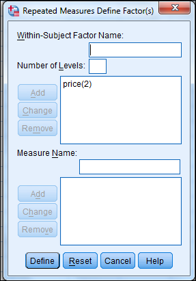
 2) When Repeated measures define Factor(s) dialog box appears type price in within subject factor name and 2 in number of levels. Press Add button and select define option.

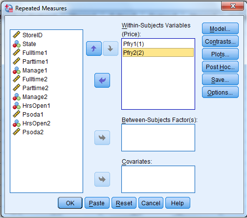
 3) Shift Click to highlight each level name then transfer them by clicking this button.
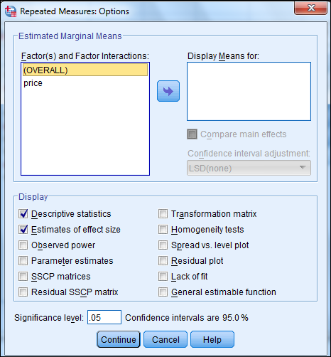
 4) Select Options and Continue buttons.
 5) Click Plots button.
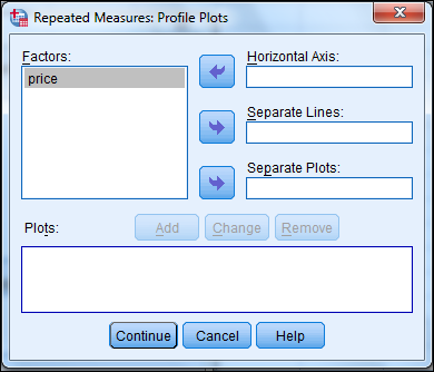 6) Click to highlight the factor name then transfer it to the Horizontal Axis, click Add button and Continue.
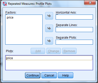 7) Click Ok to run the analysis.
The output is shown below:
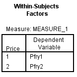
The table below shows the name given to the factor and the number of levels of the factor together with their names.
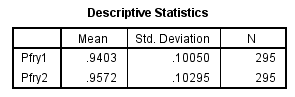
 The table below shows the mean and standard deviation of each time period.
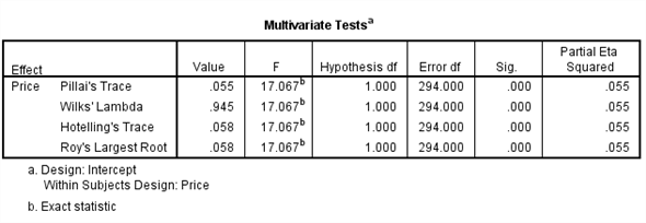
 The table below shows the
 value and its level of significance for testing the equality of means of the factor.
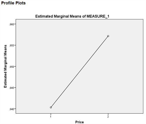 We test to determine whether there is significant change in the mean price of small fry before and after the wage rise.
The null and alternative hypotheses are,
 There is no significant change in the mean price of small fry before and after the wage rise.
 There is significant change in the mean price of small fry before and after the wage rise.
Under the null hypothesis the test statistic is defined as,
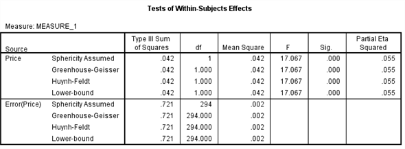
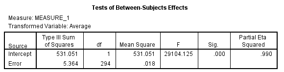
 From the output test of within subjects effects ,
The
 is 17.067
The
 value is 0.000
Here we observe that the
 value is less, so we reject the null hypothesis. Therefore, we conclude that there is significant change in the mean price of small fry before and after the wage rise.
2)
We test to determine whether the change in price of a small fry before ( Pfry1) and after ( Pfry2) the wage raise differs significantly in Pennsylvania.
Using SPSS, following is the procedure for obtaining the ANOVA output for the given data.
1) Select Analyze, general linear model and repeated measures.
 2) When Repeated measures define Factor(s) dialog box appears type price in within subject factor name and 2 in number of levels. Press Add button and select define option.
 3) Shift Click to highlight each level name then transfer them by clicking this button.

 4) Select Options and Continue buttons.
 5) Click Plots button.
 6) Click to highlight the factor name then transfer it to the Horizontal Axis, click Add button and Continue.
 7) Click Ok to run the analysis.
The output is shown below:
The table below shows the name given to the factor and the number of levels of the factor together with their names.
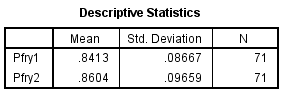
 The table below shows the mean and standard deviation of each time period.
 The table below shows the
 value and its level of significance for testing the equality of means of the factor.
 We test to determine whether there is significant change in the mean price of small fry before and after the wage rise.
The null and alternative hypotheses are,
 There is no significant change in the mean price of small fry before and after the wage rise.
 There is significant change in the mean price of small fry before and after the wage rise.
Under the null hypothesis the test statistic is defined as,
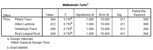
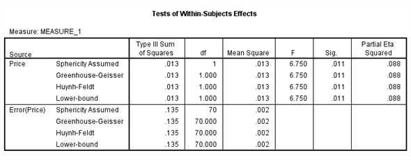
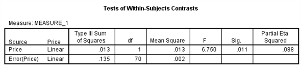
 From the output test of within subjects effects ,
The
 is 6.750
The
 value is 0.011
Here we observe that the
 value is less, so we reject the null hypothesis. Therefore, we conclude that there is significant change in the mean price of small fry before and after the wage rise.
And 1 represents New Jersey
1)
We test to determine whether the change in price of a small fry before ( Pfry1) and after ( Pfry2) the wage raise differs significantly in New Jersey.
Using SPSS, following is the procedure for obtaining the ANOVA output for the given data.
1) Select Analyze, general linear model and repeated measures.
2) When Repeated measures define Factor(s) dialog box appears type price in within subject factor name and 2 in number of levels. Press Add button and select define option. 3) Shift Click to highlight each level name then transfer them by clicking this button. 4) Select Options and Continue buttons. 5) Click Plots button. 6) Click to highlight the factor name then transfer it to the Horizontal Axis, click Add button and Continue. 7) Click Ok to run the analysis.The output is shown below:
The table below shows the name given to the factor and the number of levels of the factor together with their names.
The table below shows the mean and standard deviation of each time period. The table below shows the value and its level of significance for testing the equality of means of the factor. We test to determine whether there is significant change in the mean price of small fry before and after the wage rise.The null and alternative hypotheses are,
There is no significant change in the mean price of small fry before and after the wage rise. There is significant change in the mean price of small fry before and after the wage rise. Under the null hypothesis the test statistic is defined as,
From the output test of within subjects effects ,The
is 17.067The
value is 0.000Here we observe that the
value is less, so we reject the null hypothesis. Therefore, we conclude that there is significant change in the mean price of small fry before and after the wage rise.2)
We test to determine whether the change in price of a small fry before ( Pfry1) and after ( Pfry2) the wage raise differs significantly in Pennsylvania.
Using SPSS, following is the procedure for obtaining the ANOVA output for the given data.
1) Select Analyze, general linear model and repeated measures.
2) When Repeated measures define Factor(s) dialog box appears type price in within subject factor name and 2 in number of levels. Press Add button and select define option. 3) Shift Click to highlight each level name then transfer them by clicking this button. 4) Select Options and Continue buttons. 5) Click Plots button. 6) Click to highlight the factor name then transfer it to the Horizontal Axis, click Add button and Continue. 7) Click Ok to run the analysis.The output is shown below:
The table below shows the name given to the factor and the number of levels of the factor together with their names.
The table below shows the mean and standard deviation of each time period. The table below shows the value and its level of significance for testing the equality of means of the factor. We test to determine whether there is significant change in the mean price of small fry before and after the wage rise.The null and alternative hypotheses are,
There is no significant change in the mean price of small fry before and after the wage rise. There is significant change in the mean price of small fry before and after the wage rise. Under the null hypothesis the test statistic is defined as,
From the output test of within subjects effects ,The
is 6.750The
value is 0.011Here we observe that the
value is less, so we reject the null hypothesis. Therefore, we conclude that there is significant change in the mean price of small fry before and after the wage rise.Note: Data files for these exercises are available at the publisher's website for this text, http://www.pearsonhighered.com/stern2e.
As previously described in Exercise 1 , the file FalseRecognitionExp.sav contains the proportion of words recognized in an experiment by participants who were tested on three categories of words: words that were not presented in lists of strong associates of the missing word (variable preccnp , referred to here as condition 1); words that were presented in lists of strong associates of the presented word ( preccpp , referred to here as condition 2); or words that both were neither presented nor had any lists of strong associates presented ( preccnn , referred to here as condition 3). Determine whether the mean of condition 1 differs significantly from the mean of condition 2, and whether the mean of condition 2 differs significantly from that of condition 3. Treat these analyses as planned comparisons.
Because the A values 56,.64, and.71 correspond to small, medium, and large effect sizes, respectively, the effect size obtained for our example can be described as large. Note that because A 12 =1 A 21 , , the value A classical, rock is.28.
The outcome of the Wilcoxon signed-ranks test illustrated above can be summarized as follows:
To determine whether math performance differs when students solve problems with classical vs. rock music in the background, the number of problems solved in 20 minutes was recorded for nine randomly selected students who were exposed to four alternating 5-minute periods in which classical or rock music was played. The median number of problems solved with the classical music background was 9.00 and that with the rock music background was 12.00. This difference, tested with a Wilcoxon signed ranks test was significant, z = 1.98, p.05. For this test, the smaller sum of ranks, based on two pairs of scores, had the value of 4.00. Of the nine paired scores one pair of ranks was tied. The A value for the effect was.72, which corresponds to a large effect (Vargha and Delaney, 2000).
Exercise 1
The file FalseRecognitionExp.sav contains the proportion of words recognized in an experiment by participants who were tested on three categories of words: words that were not presented in lists of strong associates of the missing word (variable preccnp ); words that were presented in lists of strong associates of the presented word ( preccpp ); or words that both were neither presented nor had any lists of strong associates presented ( preccnn ).
1. Prepare a table that shows the means of the three variables in descending order. Include in the table each variable's standard deviation, minimum, and maximum value.
2. Present a single boxplot of the three variables. Use the variable name to label cases. What does the plot reveal about the shape of the distribution of each variable and about the presence of unusual scores
We test to determine whether the means are significantly differ.
Here we take Preccnp referred to condition1.
Preccpp referred to condition2
Preccnn referred to condition3
Using SPSS, following is the procedure for obtaining the Pairwise comparisons output for the given data.
1) Select Analyze, general linear model and repeated measures.
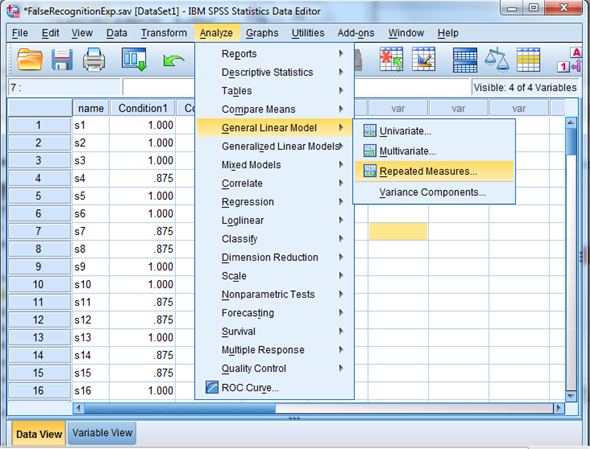 2) When Repeated measures define Factor(s) dialog box appears type time in within subject factor name and 3 in number of levels. Presss Add button and select define option.
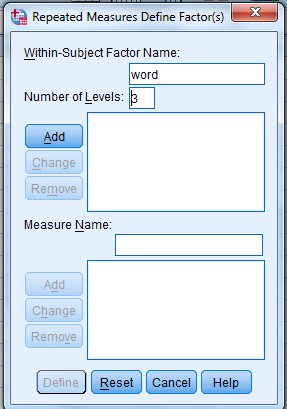
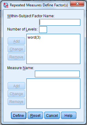 3)
3)
Shift Click to highlight each level name then transfer them by clicking this button.
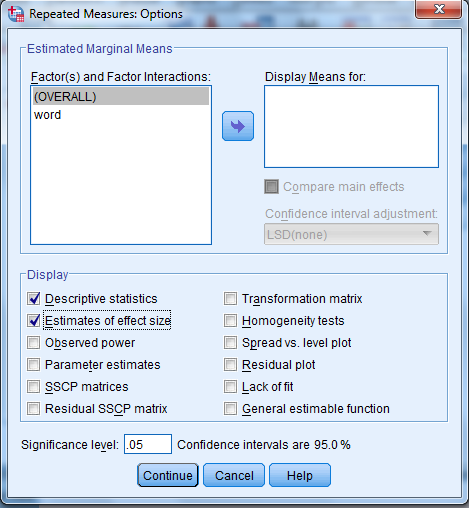
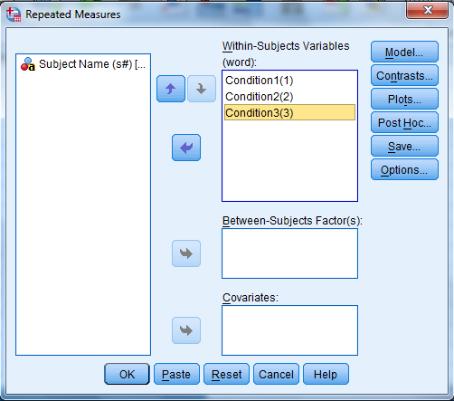 4) Select Options transfer the variable to Display means for text box, Click compare main effect, Select Sidak and Continue buttons.
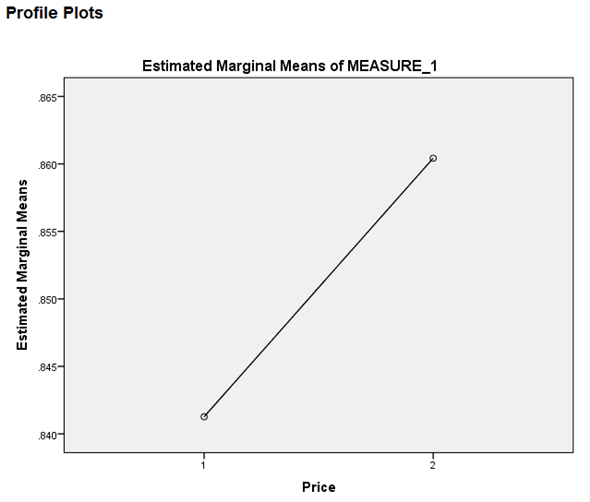
 5) Click Plots button.
 6) Click to highlight the factor name then transfer it to the Horizontal Axis, click Add button and Continue.
 7) Click Ok to run the analysis.
The output is shown below:
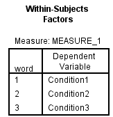
The table below shows the name given to the factor and the number of levels of the factor together with their names.
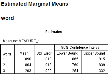
 The table below shows the mean and standard deviation of each time period.
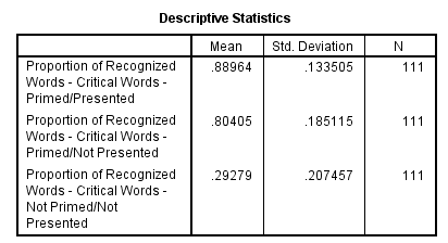
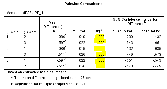 From the above output, it can be seen that the P - values for the means of condition1, condtion2 and condition3 are less.
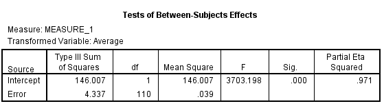
Therefore, the means of condition1 and condition2, condition1 and condition3, condition2 and condition3 are signficantly different.
Here we take Preccnp referred to condition1.
Preccpp referred to condition2
Preccnn referred to condition3
Using SPSS, following is the procedure for obtaining the Pairwise comparisons output for the given data.
1) Select Analyze, general linear model and repeated measures.
2) When Repeated measures define Factor(s) dialog box appears type time in within subject factor name and 3 in number of levels. Presss Add button and select define option. 3) Shift Click to highlight each level name then transfer them by clicking this button.
4) Select Options transfer the variable to Display means for text box, Click compare main effect, Select Sidak and Continue buttons. 5) Click Plots button. 6) Click to highlight the factor name then transfer it to the Horizontal Axis, click Add button and Continue. 7) Click Ok to run the analysis.The output is shown below:
The table below shows the name given to the factor and the number of levels of the factor together with their names.
The table below shows the mean and standard deviation of each time period. From the above output, it can be seen that the P - values for the means of condition1, condtion2 and condition3 are less.Therefore, the means of condition1 and condition2, condition1 and condition3, condition2 and condition3 are signficantly different.
Unlock Deck
Unlock for access to all 3 flashcards in this deck.


