Deck 9: More on Specification and Data Problems
Full screen (f)
Question
Use the data from JTRAIN.RAW for this exercise.
(i) Consider the simple regression model
log(scrap) = 0 + grant + u,
where scrap is the firm scrap rate and grant is a dummy variable indicating whether a firm received a job training grant. Can you think of some reasons why the unobserved factors in u might be correlated with grant
(ii) Estimate the simple regression model using the data for 1988. (You should have 54 observation s.) Does receiving a job training grant significantly lower a firm's scrap rate
(iii) Now, add as an explanatory variable log(scrap87). How does this change the estimated effect of grant Interpret the coefficient on grant. Is it statistically significant at the 5% level against the one-sided alternative H 1 : grant 0
(iv) Test the null hypothesis that the parameter on log(scrap87) is one against the two-sided alternative. Report the p-value for the test.
(v) Repeat parts (iii) and (iv), using heteroskedasticity-robust standard errors, and briefly discuss any notable differences.
(i) Consider the simple regression model
log(scrap) = 0 + grant + u,
where scrap is the firm scrap rate and grant is a dummy variable indicating whether a firm received a job training grant. Can you think of some reasons why the unobserved factors in u might be correlated with grant
(ii) Estimate the simple regression model using the data for 1988. (You should have 54 observation
s.) Does receiving a job training grant significantly lower a firm's scrap rate (iii) Now, add as an explanatory variable log(scrap87). How does this change the estimated effect of grant Interpret the coefficient on grant. Is it statistically significant at the 5% level against the one-sided alternative H 1 : grant 0
(iv) Test the null hypothesis that the parameter on log(scrap87) is one against the two-sided alternative. Report the p-value for the test.
(v) Repeat parts (iii) and (iv), using heteroskedasticity-robust standard errors, and briefly discuss any notable differences.
Question
Let math10 denote the percentage of students at a Michigan high school receiving a passing score on a standardized math test (see also Example). We are interested in estimating the effect of per student spending on math performance. A simple model is
math10 = 0 + 1 log(expend) + 2 log(enroll)+ 3 poverty + u,
where poverty is the percentage of students living in poverty.
(i) The variable lnchprg is the percentage of students eligible for the federally funded school lunch program. Why is this a sensible proxy variable for poverty
(ii) The table that follows contains OLS estimates, with and without lnchprg as an explanatory variable.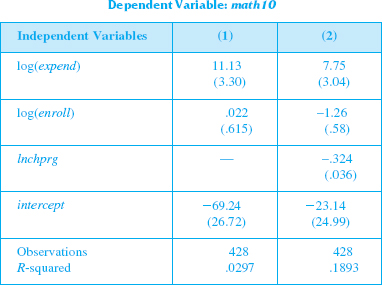
Explain why the effect of expenditures on math10 is lower in column (2) than in column (1). Is the effect in column (2) still statistically greater than zero
(iii) Does it appear that pass rates are lower at larger schools, other factors being equal Explain.
(iv) Interpret the coefficient on lnchprg in column (2).
(v) What do you make of the substantial increase in R 2 from column (1) to column (2)
Question
Use the data for the year 1990 in INFMRT.RAW for this exercise.
(i) Reestimate equation, but now include a dummy variable for the observation on the District of Columbia (called DC). Interpret the coefficient on DC and com¬ment on its size and significance. = 33.86 - 4.68 log(pcinc) + 4.15 log(physic)
(20.43) (2.60) (1.51)
_.088 log(popul)
(.287)
n = 51, R 2 =139,R 2 =.084.
(ii) Compare the estimates and standard errors from part (i) with those from equation. What do you conclude about including a dummy variable for a single observation =23.95-.57 log(pcinc)-2.74 log(physic)
(12.42) (1.64) (1.19)
+.629 log(popul)
(.191)
n = 50, R 2 =.273, 2 =.226s.
(i) Reestimate equation, but now include a dummy variable for the observation on the District of Columbia (called DC). Interpret the coefficient on DC and com¬ment on its size and significance.
= 33.86 - 4.68 log(pcinc) + 4.15 log(physic)(20.43) (2.60) (1.51)
_.088 log(popul)
(.287)
n = 51, R 2 =139,R 2 =.084.
(ii) Compare the estimates and standard errors from part (i) with those from equation. What do you conclude about including a dummy variable for a single observation
=23.95-.57 log(pcinc)-2.74 log(physic)(12.42) (1.64) (1.19)
+.629 log(popul)
(.191)
n = 50, R 2 =.273,
2 =.226s. Question
Question
Question
Question
Question
Question
Use the data in LOANAPP.RAW for this exercise.
(i) How many observations have obrat 40, that is, other debt obligations more than 40% of total income
(ii) Reestimate the model in part (iii) of Computer Exercise C7.8, excluding observa¬tions with obrat 40. What happens to the estimate and t statistic on white
(iii) Does it appear that the estimate of (3white is overly sensitive to the sample used
Use the data in LOANAPP.RAW for this exercise. The binary variable to be explained is approve, which is equal to one if a mortgage loan to an individual was approved. The key explanatory variable is white, a dummy variable equal to one if the applicant was white. The other applicants in the data set are black and Hispanic.
To test for discrimination in the mortgage loan market, a linear probability model can be used:
(i) If there is discrimination against minorities, and the appropriate factors have been controlled for, what is the sign of _1
(ii) Regress approve on white and report the results in the usual form. Interpret the coefficient on white. Is it statistically significant Is it practically large
(iii) As controls, add the variables hrat, obrat, loanprc, unem, male, married, dep, sch, cosign, chist, pubrec, mortlat1, mortlat2, and vr. What happens to the coefficient on white Is there still evidence of discrimination against nonwhites
(iv) Now, allow the effect of race to interact with the variable measuring other obligations as a percentage of income (obrat). Is the interaction term significant
(v) Using the model from part (iv), what is the effect of being white on the probability of approval when obrat _ 32, which is roughly the mean value in the sample Obtain a 95% confidence interval for this effect.
Question
Consider the simple regression model with classical measurement error, y = 0 + 1x* + u, where we have m measures on x*. Write these as z h = x* + e h , h = 1,..., m. Assume that
x* is un-correlated with u, e1,.... , em, that the measurement errors are pairwise uncorrelated,
and have the same variance, a2. Let w = (z1 +... + zm)/m be the average of the measures on x*, so that, for each observation i, w. = (z., +... + z.)/m is the average of the m measures. Let 31 be the OLS estimator from the simple regression y. on 1, w. , i = 1,..., n, using a random sample of data.
(i) Show that![Consider the simple regression model with classical measurement error, y = 0 + 1x* + u, where we have m measures on x*. Write these as z h = x* + e h , h = 1,..., m. Assume that x* is un-correlated with u, e1,.... , em, that the measurement errors are pairwise uncorrelated, and have the same variance, a2. Let w = (z1 +... + zm)/m be the average of the measures on x*, so that, for each observation i, w. = (z., +... + z.)/m is the average of the m measures. Let 31 be the OLS estimator from the simple regression y. on 1, w. , i = 1,..., n, using a random sample of data. (i) Show that [Hint: The plim of 3-1 is Cov(w,-y)/Var(w).] (ii) How does the inconsistency in 31 compare with that when only a single measure is available (that is, m = 1) What happens as m grows Comment.<div style=padding-top: 35px>](https://d2lvgg3v3hfg70.cloudfront.net/SM2712/11eb9ee2_f0f6_b70c_8edd_6309e4eff037_SM2712_00.jpg)
[Hint: The plim of 3-1 is Cov(w,-y)/Var(w).]
(ii) How does the inconsistency in 31 compare with that when only a single measure is available (that is, m = 1) What happens as m grows Comment.
x* is un-correlated with u, e1,.... , em, that the measurement errors are pairwise uncorrelated,
and have the same variance, a2. Let w = (z1 +... + zm)/m be the average of the measures on x*, so that, for each observation i, w. = (z., +... + z.)/m is the average of the m measures. Let 31 be the OLS estimator from the simple regression y. on 1, w. , i = 1,..., n, using a random sample of data.
(i) Show that
[Hint: The plim of 3-1 is Cov(w,-y)/Var(w).]
(ii) How does the inconsistency in 31 compare with that when only a single measure is available (that is, m = 1) What happens as m grows Comment.
Question
Use the data in TWOYEAR.RAW for this exercise.
(i) The variable stotal is a standardized test variable, which can act as a proxy variable for unobserved ability. Find the sample mean and standard deviation of stotal.
(ii) Run simple regressions of jc and univ on stotal. Are both college education variables statistically related to stotal Explain.
(iii) Add stotal to equation and test the hypothesis that the returns to two- and four-year colleges are the same against the alternative that the return to four-year colleges is greater. How do your findings compare with those from Section 4.4
(iv) Add stotal2 to the equation estimated in part (iii). Does a quadratic in the test score variable seem necessary
(v) Add the interaction terms stotal-jc and stotal-univ to the equation from part (iii). Are these terms jointly significant
(vi) What would be your final model that controls for ability through the use of stotal Justify your answer.
Question
In this exercise, you are to compare OLS and LAD estimates of the effects of 401(k) plan eligibility on net financial assets. The model is 
(i) Use the data in 401KSUBS.RAW to estimate the equation by OLS and report the results in the usual form. Interpret the coefficient on e401k.
(ii) Use the OLS residuals to test for heteroskedasticity using the Breusch-Pagan test. Is u independent of the explanatory variables
(iii) Estimate the equation by LAD and report the results in the same form as for OLS. Interpret the LAD estimate of 6.
(iv) Reconcile your findings from parts (i) and (iii).
Question
Apply RESET from equation to the model estimated in Computer Exercise. Is there evidence of functional form misspecification in the equation
(ii) Compute a heteroskedasticity-robust form of RESET. Does your conclusion from part (i) change
y = 0 + 1 x 1 +… + k x k + 1 2 + 2
2 + 2  3 +error.
In Problem 4.2, we added the return on the firm's stock, ros, to a model explaining CEO salary; ros turned out to be insignificant. Now, define a dummy variable, rosneg, which is equal to one if ros _ 0 and equal to zero if ros _ 0. Use CEOSAL1.RAW to estimate the model
Discuss the interpretation and statistical significance of 3.
3.
(ii) Compute a heteroskedasticity-robust form of RESET. Does your conclusion from part (i) change
y = 0 + 1 x 1 +… + k x k + 1
2 + 2 3 +error.In Problem 4.2, we added the return on the firm's stock, ros, to a model explaining CEO salary; ros turned out to be insignificant. Now, define a dummy variable, rosneg, which is equal to one if ros _ 0 and equal to zero if ros _ 0. Use CEOSAL1.RAW to estimate the model
Discuss the interpretation and statistical significance of
3. Question
You need to use two data sets for this exercise, JTRAIN2.RAW and JTRAIN3.RAW. The former is the outcome of a job training experiment. The file JTRAIN3.RAW contains observational data, where individuals themselves largely determine whether they participate in job training. The data sets cover the same time period.
(i) In the data set JTRAIN2.RAW, what fraction of the men received job training What is the fraction in JTRAIN3.RAW Why do you think there is such a big difference
(ii) Using JTRAIN2.RAW, run a simple regression of re78 on train. What is the estimated effect of participating in job training on real earnings
(iii) Now add as controls to the regression in part (ii) the variables re74, re75, educ, age, black, and hisp. Does the estimated effect of job training on re78 change much How come (Hint: Remember that these are experimental data.)
(iv) Do the regressions in parts (ii) and (iii) using the data in JTRAIN3.RAW, reporting only the estimated coefficients on train, along with their t statistics. What is the effect now of controlling for the extra factors, and why
(v) Define avgre = (re74 + re75)/2. Find the sample averages, standard deviations, and minimum and maximum values in the two data sets. Are these data sets representative of the same populations in 1978
(vi) Almost 96% of men in the data set JTRAIN2.RAW have avgre less than $10,000. Using only these men, run the regression re78 on train,re74,re75,educ,age,black,hisp and report the training estimate and its t statistic. Run the same regression for JTRAIN3.RAW, using only men with avgre 10. For the subsample of low-income men, how do the estimated training effects compare across the experimental and non-experimental data sets
(vii) Now use each data set to run the simple regression re78 on train, but only for men who were unemployed in 1974 and 1975. How do the training estimates compare now
(viii) Using your findings from the previous regressions, discuss the potential importance of having comparable populations underlying comparisons of experimental and non-experimental estimates.
(i) In the data set JTRAIN2.RAW, what fraction of the men received job training What is the fraction in JTRAIN3.RAW Why do you think there is such a big difference
(ii) Using JTRAIN2.RAW, run a simple regression of re78 on train. What is the estimated effect of participating in job training on real earnings
(iii) Now add as controls to the regression in part (ii) the variables re74, re75, educ, age, black, and hisp. Does the estimated effect of job training on re78 change much How come (Hint: Remember that these are experimental data.)
(iv) Do the regressions in parts (ii) and (iii) using the data in JTRAIN3.RAW, reporting only the estimated coefficients on train, along with their t statistics. What is the effect now of controlling for the extra factors, and why
(v) Define avgre = (re74 + re75)/2. Find the sample averages, standard deviations, and minimum and maximum values in the two data sets. Are these data sets representative of the same populations in 1978
(vi) Almost 96% of men in the data set JTRAIN2.RAW have avgre less than $10,000. Using only these men, run the regression re78 on train,re74,re75,educ,age,black,hisp and report the training estimate and its t statistic. Run the same regression for JTRAIN3.RAW, using only men with avgre
10. For the subsample of low-income men, how do the estimated training effects compare across the experimental and non-experimental data sets (vii) Now use each data set to run the simple regression re78 on train, but only for men who were unemployed in 1974 and 1975. How do the training estimates compare now
(viii) Using your findings from the previous regressions, discuss the potential importance of having comparable populations underlying comparisons of experimental and non-experimental estimates.
Question
Question
Question
Question
Question
Let us modify Computer Exercise C8.4 by using voting outcomes in 1990 for incumbents who were elected in 1988. Candidate A was elected in 1988 and was seeking reelection in 1990; voteA90 is Candidate A's share of the two-party vote in 1990. The 1988 voting share of Candidate A is used as a proxy variable for quality of the candidate. All other variables are for the 1990 election. The following equations were estimated, using the data in VOTE2.RAW:  = 75.71 +.312 prtystrA + 4.93 democA
(9.25) (.046) (1.01)
-.929 log(expendA) - 1.950 log(expendB)
(.684) (.281)
n = 186, R 2 =.495, R 2 =.483,
and = 70.81 +.282 prtystrA + 4.52 democA
(10.01) (.052) (1.06)
-.839 log(expendA) - 1.846 log(expendB) +.067 voteA88
(.687) (.292) (.053)
n = 186, R 2 =.499, 2 =.485.
(i) Interpret the coefficient on voteA88 and discuss its statistical significance.
(ii) Does adding voteA88 have much effect on the other coefficients
= 75.71 +.312 prtystrA + 4.93 democA(9.25) (.046) (1.01)
-.929 log(expendA) - 1.950 log(expendB)
(.684) (.281)
n = 186, R 2 =.495, R 2 =.483,
and
= 70.81 +.282 prtystrA + 4.52 democA(10.01) (.052) (1.06)
-.839 log(expendA) - 1.846 log(expendB) +.067 voteA88
(.687) (.292) (.053)
n = 186, R 2 =.499,
2 =.485.(i) Interpret the coefficient on voteA88 and discuss its statistical significance.
(ii) Does adding voteA88 have much effect on the other coefficients

Unlock Deck
Sign up to unlock the cards in this deck!
Unlock Deck
Unlock Deck
1/19
Play
Full screen (f)
Deck 9: More on Specification and Data Problems
1
Use the data from JTRAIN.RAW for this exercise.
(i) Consider the simple regression model
log(scrap) = 0 + grant + u,
where scrap is the firm scrap rate and grant is a dummy variable indicating whether a firm received a job training grant. Can you think of some reasons why the unobserved factors in u might be correlated with grant
(ii) Estimate the simple regression model using the data for 1988. (You should have 54 observation s.) Does receiving a job training grant significantly lower a firm's scrap rate
(iii) Now, add as an explanatory variable log(scrap87). How does this change the estimated effect of grant Interpret the coefficient on grant. Is it statistically significant at the 5% level against the one-sided alternative H 1 : grant 0
(iv) Test the null hypothesis that the parameter on log(scrap87) is one against the two-sided alternative. Report the p-value for the test.
(v) Repeat parts (iii) and (iv), using heteroskedasticity-robust standard errors, and briefly discuss any notable differences.
(i) Consider the simple regression model
log(scrap) = 0 + grant + u,
where scrap is the firm scrap rate and grant is a dummy variable indicating whether a firm received a job training grant. Can you think of some reasons why the unobserved factors in u might be correlated with grant
(ii) Estimate the simple regression model using the data for 1988. (You should have 54 observation
s.) Does receiving a job training grant significantly lower a firm's scrap rate (iii) Now, add as an explanatory variable log(scrap87). How does this change the estimated effect of grant Interpret the coefficient on grant. Is it statistically significant at the 5% level against the one-sided alternative H 1 : grant 0
(iv) Test the null hypothesis that the parameter on log(scrap87) is one against the two-sided alternative. Report the p-value for the test.
(v) Repeat parts (iii) and (iv), using heteroskedasticity-robust standard errors, and briefly discuss any notable differences.
(i)
In the simple regression model The unobserved factors in
  might be correlated with
  due some important omitted variables in the regression model that exhibit significant degree of correlation with
  Such omitted variables could be the factors that effects both
  and
and  such as the ability and education of the employees and other firm characteristics such as degree of sophistication of operations, level of attrition-rate, the nature of the firm-priority sector, profit-making or departmental undertaking etc
(ii)
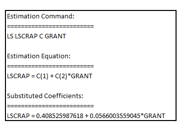
Estimating the simple regression model using the data for 1988, the result is:
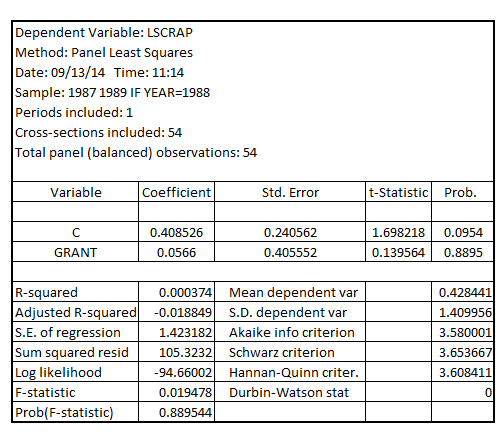
 The coefficient of
  is 0.0566 which is positive, but not statistically significant at 5% level of significance as one-tailed p-value corresponding to its coefficient is 0.44475 (0.8895 divided by 2) which is greater than the critical p-value of 0.05 at 5% level of significance
Hence, it would not be possible to concluded if receiving a job training grant significantly lower a firm's scrap rate
(iii)
On adding the explanatory variable to the model, the model becomes:
  Estimating the regression model using the data for 1988, the result is:
 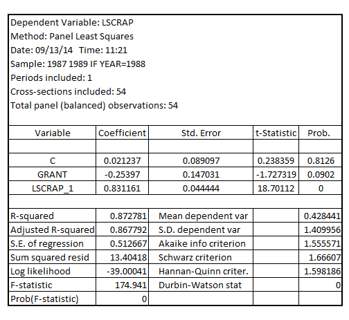 The coefficient of
  is -0.25397 which is negative
It is interpreted as the scrap rate would reduce by 25.397% if the firm received the job training grant on an average
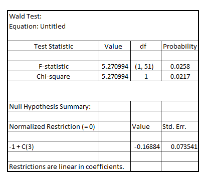
On testing for the significance of the coefficient of , the Wald-test results in:
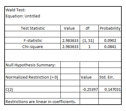 The (one-tailed) p-value of F-statistic is 0.04510 (0.0902 divided by 2) indicating that the coefficient of
  is statistically significant at 5% level of significance thereby implying that receiving a job training grant significantly lower a firm's scrap rate
(iv)
On testing the significance of the coefficient of using Wald-test, the result is:
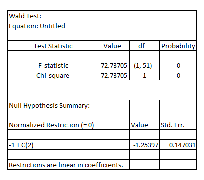 Since, the p-value of F-statistic is 0.0000 which is less than the critical p-value of 0.05 at 5% level of significance, it is indicated that the coefficient of
  is statistically significant at 5% level of significance
(v)
On adding the explanatory variable to the model, the model becomes:
  Estimating the regression model using the data for 1988 assuming heteroscedasticity-robust standard errors, the result is:
 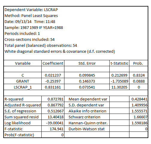 The coefficient of
  is -0.25397 which is negative
It is interpreted as the scrap rate would reduce by 25.397% if the firm received the job training grant on an average
On testing for the significance of the coefficient of , the Wald-test results in:
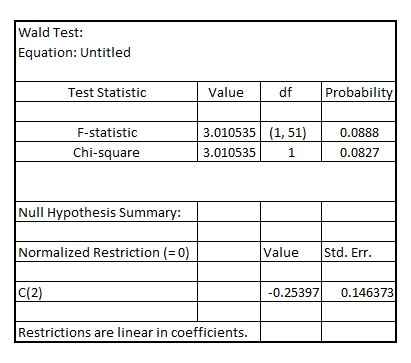 The (one-tailed) p-value of F-statistic is 0.0444 (0.0888 divided by 2) indicating that the coefficient of
  is statistically significant at 5% level of significance thereby implying that receiving a job training grant significantly lower a firm's scrap rate
On testing the significance of the coefficient of using Wald-test, the result is:
 Since, the p-value of F-statistic is 0.0258 which is less than the critical p-value of 0.05 at 5% level of significance, it is indicated that the coefficient of
  is statistically significant at 5% level of significance
On comparing the results based on usual OLS standard errors and heteroscedasticity-robust standard error for the model The key points are:
1) The p-value (one-tailed) of the coefficient of decreased from 0.04510 (under usual OLS standard error) to 0.0444(under heteroscedasticity-robust standard error)
2) The p-value (two-tailed) for the test of significance of the coefficient on being equal to 1 increased from 0.0000 (under usual OLS standard error) to 0.0258 (under heteroscedasticity-robust standard error)
In the simple regression model
The unobserved factors in might be correlated with due some important omitted variables in the regression model that exhibit significant degree of correlation with Such omitted variables could be the factors that effects both and such as the ability and education of the employees and other firm characteristics such as degree of sophistication of operations, level of attrition-rate, the nature of the firm-priority sector, profit-making or departmental undertaking etc(ii)
Estimating the simple regression model using the data for 1988, the result is:
The coefficient of is 0.0566 which is positive, but not statistically significant at 5% level of significance as one-tailed p-value corresponding to its coefficient is 0.44475 (0.8895 divided by 2) which is greater than the critical p-value of 0.05 at 5% level of significanceHence, it would not be possible to concluded if receiving a job training grant significantly lower a firm's scrap rate
(iii)
On adding the explanatory variable
to the model, the model becomes: Estimating the regression model using the data for 1988, the result is: The coefficient of is -0.25397 which is negative It is interpreted as the scrap rate would reduce by 25.397% if the firm received the job training grant on an average
On testing for the significance of the coefficient of
, the Wald-test results in: The (one-tailed) p-value of F-statistic is 0.04510 (0.0902 divided by 2) indicating that the coefficient of is statistically significant at 5% level of significance thereby implying that receiving a job training grant significantly lower a firm's scrap rate(iv)
On testing the significance of the coefficient of
using Wald-test, the result is: Since, the p-value of F-statistic is 0.0000 which is less than the critical p-value of 0.05 at 5% level of significance, it is indicated that the coefficient of is statistically significant at 5% level of significance(v)
On adding the explanatory variable
to the model, the model becomes: Estimating the regression model using the data for 1988 assuming heteroscedasticity-robust standard errors, the result is: The coefficient of is -0.25397 which is negative It is interpreted as the scrap rate would reduce by 25.397% if the firm received the job training grant on an average
On testing for the significance of the coefficient of
, the Wald-test results in: The (one-tailed) p-value of F-statistic is 0.0444 (0.0888 divided by 2) indicating that the coefficient of is statistically significant at 5% level of significance thereby implying that receiving a job training grant significantly lower a firm's scrap rateOn testing the significance of the coefficient of
using Wald-test, the result is: Since, the p-value of F-statistic is 0.0258 which is less than the critical p-value of 0.05 at 5% level of significance, it is indicated that the coefficient of is statistically significant at 5% level of significanceOn comparing the results based on usual OLS standard errors and heteroscedasticity-robust standard error for the model
The key points are:1) The p-value (one-tailed) of the coefficient of
decreased from 0.04510 (under usual OLS standard error) to 0.0444(under heteroscedasticity-robust standard error)2) The p-value (two-tailed) for the test of significance of the coefficient on
being equal to 1 increased from 0.0000 (under usual OLS standard error) to 0.0258 (under heteroscedasticity-robust standard error) 2
Let math10 denote the percentage of students at a Michigan high school receiving a passing score on a standardized math test (see also Example). We are interested in estimating the effect of per student spending on math performance. A simple model is
math10 = 0 + 1 log(expend) + 2 log(enroll)+ 3 poverty + u,
where poverty is the percentage of students living in poverty.
(i) The variable lnchprg is the percentage of students eligible for the federally funded school lunch program. Why is this a sensible proxy variable for poverty
(ii) The table that follows contains OLS estimates, with and without lnchprg as an explanatory variable.
Explain why the effect of expenditures on math10 is lower in column (2) than in column (1). Is the effect in column (2) still statistically greater than zero
(iii) Does it appear that pass rates are lower at larger schools, other factors being equal Explain.
(iv) Interpret the coefficient on lnchprg in column (2).
(v) What do you make of the substantial increase in R 2 from column (1) to column (2)
math10 = 0 + 1 log(expend) + 2 log(enroll)+ 3 poverty + u,
where poverty is the percentage of students living in poverty.
(i) The variable lnchprg is the percentage of students eligible for the federally funded school lunch program. Why is this a sensible proxy variable for poverty
(ii) The table that follows contains OLS estimates, with and without lnchprg as an explanatory variable.
Explain why the effect of expenditures on math10 is lower in column (2) than in column (1). Is the effect in column (2) still statistically greater than zero
(iii) Does it appear that pass rates are lower at larger schools, other factors being equal Explain.
(iv) Interpret the coefficient on lnchprg in column (2).
(v) What do you make of the substantial increase in R 2 from column (1) to column (2)
Consider the model, the result of which is given in column (1) and column (2) 
 It shall be noted that
  is used as the proxy variable for
  The column (1) is the result of the model without
  The column (2) is the result of the model with
  (i)
(i)
Considering as the percentage of students eligible for the federally funded school lunch program, it is considered to be a sensible proxy variable for
  .This is because, the federally funded school lunch program is aimed at promoting the children of the families below poverty line to attend school. In order to ensure family support as well as the interest of such children to go to school, this program ensures that the children of such families get a free lunch meal
(ii)
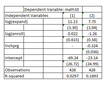
The effect of expenditures on is measured by the coefficient of
  The coefficient of
  is 11.13 in column (1) which is higher than the coefficient of
  at 7.75 in column (2)
The effect of expenditure is lower in column (2) than in column (1). This is because, is included as an explanatory variable in the model, the result of which is shown in column (2)
The explanatory variable is omitted in the model the result of which is shown in column (1)
The variable is negatively related to
  and given that the coefficient of
  is negative, the omission of the variable
  would result in upward bias in the estimate of the coefficient of
  Hence, the effects of expenditures on
  is lower in column (2) than in column (1)
In order to test for the statistical significance of the effects of expenditure on in column (2), it would be appropriate to conduct the t-test
  The effects of expenditures on
  is equal to zero
  The effects of expenditures on
  is greater than zero
The result is: The critical (one-tailed) t-statistic at 5% level of significance for
  is1.645, which is less than the actual t-statistic of 2.5493, the effects of expenditures on
  in column (2) is statistically significantly greater than zero at 5% level of significance
(iii)
The largeness of the school is determined by . Higher the value of
  , larger the school is.
The coefficient of is -1.26 in column (2) indicating that an increase of 10% in
  , results in decrease of
  by 0.126% point, thereby indicating that the pass rate
  are lower at larger schools, other factors being equal.
(iv)
The coefficient of in column (2) is -0.324, indicating that 1% point increase in
  (the percentage of students eligible for the federally funded school lunch program)results in 0.324% point decrease in
  ,other factors being equal
(v)
The R-squared in column (1) is 0.0297 whereas it is 0.1893 in column (2)
The R-squared value in column (1) indicates that the model without could explain 2.97% of the variations in
  where as the R-squared value in column (2) indicates that the model with
  could explain 18.93% of the variations in
  That means, the inclusion of
  in the model increases the explanatory power of the model indicating that
  is more important a determinant of
  than
than  or
or 
It shall be noted that is used as the proxy variable for The column (1) is the result of the model without The column (2) is the result of the model with (i)Considering
as the percentage of students eligible for the federally funded school lunch program, it is considered to be a sensible proxy variable for .This is because, the federally funded school lunch program is aimed at promoting the children of the families below poverty line to attend school. In order to ensure family support as well as the interest of such children to go to school, this program ensures that the children of such families get a free lunch meal (ii)
The effect of expenditures on
is measured by the coefficient of The coefficient of is 11.13 in column (1) which is higher than the coefficient of at 7.75 in column (2)The effect of expenditure is lower in column (2) than in column (1). This is because,
is included as an explanatory variable in the model, the result of which is shown in column (2)The explanatory variable
is omitted in the model the result of which is shown in column (1)The variable
is negatively related to and given that the coefficient of is negative, the omission of the variable would result in upward bias in the estimate of the coefficient of Hence, the effects of expenditures on is lower in column (2) than in column (1)In order to test for the statistical significance of the effects of expenditure on
in column (2), it would be appropriate to conduct the t-test The effects of expenditures on is equal to zero The effects of expenditures on is greater than zeroThe result is:
The critical (one-tailed) t-statistic at 5% level of significance for is1.645, which is less than the actual t-statistic of 2.5493, the effects of expenditures on in column (2) is statistically significantly greater than zero at 5% level of significance(iii)
The largeness of the school is determined by
. Higher the value of , larger the school is.The coefficient of
is -1.26 in column (2) indicating that an increase of 10% in , results in decrease of by 0.126% point, thereby indicating that the pass rate are lower at larger schools, other factors being equal.(iv)
The coefficient of
in column (2) is -0.324, indicating that 1% point increase in (the percentage of students eligible for the federally funded school lunch program)results in 0.324% point decrease in ,other factors being equal(v)
The R-squared in column (1) is 0.0297 whereas it is 0.1893 in column (2)
The R-squared value in column (1) indicates that the model without
could explain 2.97% of the variations in where as the R-squared value in column (2) indicates that the model with could explain 18.93% of the variations in That means, the inclusion of in the model increases the explanatory power of the model indicating that is more important a determinant of than or 3
Use the data for the year 1990 in INFMRT.RAW for this exercise.
(i) Reestimate equation, but now include a dummy variable for the observation on the District of Columbia (called DC). Interpret the coefficient on DC and com¬ment on its size and significance. = 33.86 - 4.68 log(pcinc) + 4.15 log(physic)
(20.43) (2.60) (1.51)
_.088 log(popul)
(.287)
n = 51, R 2 =139,R 2 =.084.
(ii) Compare the estimates and standard errors from part (i) with those from equation. What do you conclude about including a dummy variable for a single observation =23.95-.57 log(pcinc)-2.74 log(physic)
(12.42) (1.64) (1.19)
+.629 log(popul)
(.191)
n = 50, R 2 =.273, 2 =.226s.
(i) Reestimate equation, but now include a dummy variable for the observation on the District of Columbia (called DC). Interpret the coefficient on DC and com¬ment on its size and significance.
= 33.86 - 4.68 log(pcinc) + 4.15 log(physic)(20.43) (2.60) (1.51)
_.088 log(popul)
(.287)
n = 51, R 2 =139,R 2 =.084.
(ii) Compare the estimates and standard errors from part (i) with those from equation. What do you conclude about including a dummy variable for a single observation
=23.95-.57 log(pcinc)-2.74 log(physic)(12.42) (1.64) (1.19)
+.629 log(popul)
(.191)
n = 50, R 2 =.273,
2 =.226s.(i)
Using the data for the year 1990 and estimating the model with the inclusion of a dummy variable for the observation on the District of Columbia (called ), the result is:
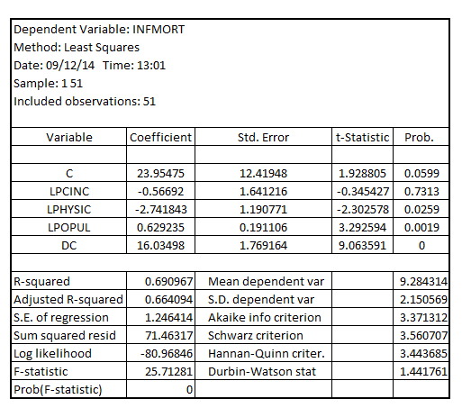
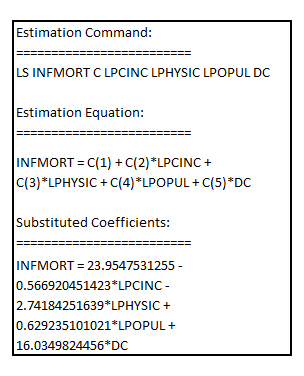 The coefficient of
  is 16.03498
It is interpreted as the infant mortality rate being 16.03498 for the State of District of Columbia
(ii)
The equation (9.44) of the example 9.10 is of the form: This regression result is based on set of 50 observations from the year 1990 data after excluding the single observation of the State of District of Columbia
On comparing the estimates and the standard error of the equation (9.44) with that of the model given by: The result is:
 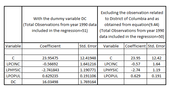 It shall be noted that corrected to two decimal places, the coefficients estimates and the standard error of the equation (9.44) are same as that obtained from the year 1990 data based model given by
  It shall be noted that there is only one observation related to
  in the data corresponding to the year 1990 out of the set of 51 observations, hence, it can be concluded that including a dummy variable for a single observation yield identical results vis-à-vis excluding the dummy variable for that single observation as far as the coefficient estimates and their respective standard error is considered
Using the data for the year 1990 and estimating the model with the inclusion of a dummy variable for the observation on the District of Columbia (called
), the result is: The coefficient of is 16.03498It is interpreted as the infant mortality rate being 16.03498 for the State of District of Columbia
(ii)
The equation (9.44) of the example 9.10 is of the form:
This regression result is based on set of 50 observations from the year 1990 data after excluding the single observation of the State of District of ColumbiaOn comparing the estimates and the standard error of the equation (9.44) with that of the model given by:
The result is: It shall be noted that corrected to two decimal places, the coefficients estimates and the standard error of the equation (9.44) are same as that obtained from the year 1990 data based model given by It shall be noted that there is only one observation related to in the data corresponding to the year 1990 out of the set of 51 observations, hence, it can be concluded that including a dummy variable for a single observation yield identical results vis-à-vis excluding the dummy variable for that single observation as far as the coefficient estimates and their respective standard error is considered 4
The following equation explains weekly hours of television viewing by a child in terms of the child's age, mother's education, father's education, and number of siblings:
tvhours* = 0 + 1 age + 2 age 2 + 3 motheduc + 4 fatheduc + 5 sibs + u.
We are worried that tvhours* is measured with error in our survey. Let tvhours denote the reported hours of television viewing per week.
(i) What do the classical errors-in-variables (CEV) assumptions require in this application
(ii) Do you think the CEV assumptions are likely to hold Explain.
(vii) Now use each data set to run the simple regression re78 on train, but only for men who were unemployed in 1974 and 1975. How do the training estimates compare now
(viii) Using your findings from the previous regressions, discuss the potential importance of having comparable populations underlying comparisons of experimental and non-experimental estimates.
Unlock Deck
Unlock for access to all 19 flashcards in this deck.
Unlock Deck
k this deck
5
Use the data in RDCHEM.RAW to further examine the effects of outliers on OLS estimates and to see how LAD is less sensitive to outliers. The model is
rdintens = 0 + 1 sales + 2 sales 2 + 3 profmarg + u,
where you should first change sales to be in billions of dollars to make the estimates easier to interpret.
(i) Estimate the above equation by OLS, both with and without the firm having annual sales of almost $40 billion. Discuss any notable differences in the estimated coefficients.
(ii) Estimate the same equation by LAD, again with and without the largest firm. Discuss any important differences in estimated coefficients.
(iii) Based on your findings in (i) and (ii), would you say OLS or LAD is more resilient to outliers
Unlock Deck
Unlock for access to all 19 flashcards in this deck.
Unlock Deck
k this deck
6
In Example, we estimated a model relating number of campus crimes to student enrollment for a sample of colleges. The sample we used was not a random sample of colleges in the United States, because many schools in 1992 did not report campus crimes. Do you think that college failure to report crimes can be viewed as exogenous sample selection Explain.
Unlock Deck
Unlock for access to all 19 flashcards in this deck.
Unlock Deck
k this deck
7
Redo Example by dropping schools where teacher benefits are less than 1% of salary.
(i) How many observations are lost
(ii) Does dropping these observations have any important effects on the estimated
tradeoff
(i) How many observations are lost
(ii) Does dropping these observations have any important effects on the estimated
tradeoff
Unlock Deck
Unlock for access to all 19 flashcards in this deck.
Unlock Deck
k this deck
8
In the model, show that OLS consistently estimates a and if a. is uncorrelated with x. and b. is uncorrelated with x. and x2 , which are weaker assumptions than (9.19). [Hint: Write the equation as in and recall from Chapter 5 that sufficient for consistency of OLS for the intercept and slope is E(ui) = 0 and Cov(xi, ui) = 0.]
Unlock Deck
Unlock for access to all 19 flashcards in this deck.
Unlock Deck
k this deck
9
Use the data in LOANAPP.RAW for this exercise.
(i) How many observations have obrat 40, that is, other debt obligations more than 40% of total income
(ii) Reestimate the model in part (iii) of Computer Exercise C7.8, excluding observa¬tions with obrat 40. What happens to the estimate and t statistic on white
(iii) Does it appear that the estimate of (3white is overly sensitive to the sample used
Use the data in LOANAPP.RAW for this exercise. The binary variable to be explained is approve, which is equal to one if a mortgage loan to an individual was approved. The key explanatory variable is white, a dummy variable equal to one if the applicant was white. The other applicants in the data set are black and Hispanic.
To test for discrimination in the mortgage loan market, a linear probability model can be used:
(i) If there is discrimination against minorities, and the appropriate factors have been controlled for, what is the sign of _1
(ii) Regress approve on white and report the results in the usual form. Interpret the coefficient on white. Is it statistically significant Is it practically large
(iii) As controls, add the variables hrat, obrat, loanprc, unem, male, married, dep, sch, cosign, chist, pubrec, mortlat1, mortlat2, and vr. What happens to the coefficient on white Is there still evidence of discrimination against nonwhites
(iv) Now, allow the effect of race to interact with the variable measuring other obligations as a percentage of income (obrat). Is the interaction term significant
(v) Using the model from part (iv), what is the effect of being white on the probability of approval when obrat _ 32, which is roughly the mean value in the sample Obtain a 95% confidence interval for this effect.
(i) How many observations have obrat 40, that is, other debt obligations more than 40% of total income
(ii) Reestimate the model in part (iii) of Computer Exercise C7.8, excluding observa¬tions with obrat 40. What happens to the estimate and t statistic on white
(iii) Does it appear that the estimate of (3white is overly sensitive to the sample used
Use the data in LOANAPP.RAW for this exercise. The binary variable to be explained is approve, which is equal to one if a mortgage loan to an individual was approved. The key explanatory variable is white, a dummy variable equal to one if the applicant was white. The other applicants in the data set are black and Hispanic.
To test for discrimination in the mortgage loan market, a linear probability model can be used:
(i) If there is discrimination against minorities, and the appropriate factors have been controlled for, what is the sign of _1
(ii) Regress approve on white and report the results in the usual form. Interpret the coefficient on white. Is it statistically significant Is it practically large
(iii) As controls, add the variables hrat, obrat, loanprc, unem, male, married, dep, sch, cosign, chist, pubrec, mortlat1, mortlat2, and vr. What happens to the coefficient on white Is there still evidence of discrimination against nonwhites
(iv) Now, allow the effect of race to interact with the variable measuring other obligations as a percentage of income (obrat). Is the interaction term significant
(v) Using the model from part (iv), what is the effect of being white on the probability of approval when obrat _ 32, which is roughly the mean value in the sample Obtain a 95% confidence interval for this effect.
Unlock Deck
Unlock for access to all 19 flashcards in this deck.
Unlock Deck
k this deck
10
Consider the simple regression model with classical measurement error, y = 0 + 1x* + u, where we have m measures on x*. Write these as z h = x* + e h , h = 1,..., m. Assume that
x* is un-correlated with u, e1,.... , em, that the measurement errors are pairwise uncorrelated,
and have the same variance, a2. Let w = (z1 +... + zm)/m be the average of the measures on x*, so that, for each observation i, w. = (z., +... + z.)/m is the average of the m measures. Let 31 be the OLS estimator from the simple regression y. on 1, w. , i = 1,..., n, using a random sample of data.
(i) Show that
[Hint: The plim of 3-1 is Cov(w,-y)/Var(w).]
(ii) How does the inconsistency in 31 compare with that when only a single measure is available (that is, m = 1) What happens as m grows Comment.
Unlock Deck
Unlock for access to all 19 flashcards in this deck.
Unlock Deck
k this deck
11
Use the data in TWOYEAR.RAW for this exercise.
(i) The variable stotal is a standardized test variable, which can act as a proxy variable for unobserved ability. Find the sample mean and standard deviation of stotal.
(ii) Run simple regressions of jc and univ on stotal. Are both college education variables statistically related to stotal Explain.
(iii) Add stotal to equation and test the hypothesis that the returns to two- and four-year colleges are the same against the alternative that the return to four-year colleges is greater. How do your findings compare with those from Section 4.4
(iv) Add stotal2 to the equation estimated in part (iii). Does a quadratic in the test score variable seem necessary
(v) Add the interaction terms stotal-jc and stotal-univ to the equation from part (iii). Are these terms jointly significant
(vi) What would be your final model that controls for ability through the use of stotal Justify your answer.
(i) The variable stotal is a standardized test variable, which can act as a proxy variable for unobserved ability. Find the sample mean and standard deviation of stotal.
(ii) Run simple regressions of jc and univ on stotal. Are both college education variables statistically related to stotal Explain.
(iii) Add stotal to equation and test the hypothesis that the returns to two- and four-year colleges are the same against the alternative that the return to four-year colleges is greater. How do your findings compare with those from Section 4.4
(iv) Add stotal2 to the equation estimated in part (iii). Does a quadratic in the test score variable seem necessary
(v) Add the interaction terms stotal-jc and stotal-univ to the equation from part (iii). Are these terms jointly significant
(vi) What would be your final model that controls for ability through the use of stotal Justify your answer.
Unlock Deck
Unlock for access to all 19 flashcards in this deck.
Unlock Deck
k this deck
12
In this exercise, you are to compare OLS and LAD estimates of the effects of 401(k) plan eligibility on net financial assets. The model is
(i) Use the data in 401KSUBS.RAW to estimate the equation by OLS and report the results in the usual form. Interpret the coefficient on e401k.
(ii) Use the OLS residuals to test for heteroskedasticity using the Breusch-Pagan test. Is u independent of the explanatory variables
(iii) Estimate the equation by LAD and report the results in the same form as for OLS. Interpret the LAD estimate of 6.
(iv) Reconcile your findings from parts (i) and (iii).
Unlock Deck
Unlock for access to all 19 flashcards in this deck.
Unlock Deck
k this deck
13
Apply RESET from equation to the model estimated in Computer Exercise. Is there evidence of functional form misspecification in the equation
(ii) Compute a heteroskedasticity-robust form of RESET. Does your conclusion from part (i) change
y = 0 + 1 x 1 +… + k x k + 1 2 + 2 3 +error.
In Problem 4.2, we added the return on the firm's stock, ros, to a model explaining CEO salary; ros turned out to be insignificant. Now, define a dummy variable, rosneg, which is equal to one if ros _ 0 and equal to zero if ros _ 0. Use CEOSAL1.RAW to estimate the model
Discuss the interpretation and statistical significance of 3.
(ii) Compute a heteroskedasticity-robust form of RESET. Does your conclusion from part (i) change
y = 0 + 1 x 1 +… + k x k + 1
2 + 2 3 +error.In Problem 4.2, we added the return on the firm's stock, ros, to a model explaining CEO salary; ros turned out to be insignificant. Now, define a dummy variable, rosneg, which is equal to one if ros _ 0 and equal to zero if ros _ 0. Use CEOSAL1.RAW to estimate the model
Discuss the interpretation and statistical significance of
3. Unlock Deck
Unlock for access to all 19 flashcards in this deck.
Unlock Deck
k this deck
14
You need to use two data sets for this exercise, JTRAIN2.RAW and JTRAIN3.RAW. The former is the outcome of a job training experiment. The file JTRAIN3.RAW contains observational data, where individuals themselves largely determine whether they participate in job training. The data sets cover the same time period.
(i) In the data set JTRAIN2.RAW, what fraction of the men received job training What is the fraction in JTRAIN3.RAW Why do you think there is such a big difference
(ii) Using JTRAIN2.RAW, run a simple regression of re78 on train. What is the estimated effect of participating in job training on real earnings
(iii) Now add as controls to the regression in part (ii) the variables re74, re75, educ, age, black, and hisp. Does the estimated effect of job training on re78 change much How come (Hint: Remember that these are experimental data.)
(iv) Do the regressions in parts (ii) and (iii) using the data in JTRAIN3.RAW, reporting only the estimated coefficients on train, along with their t statistics. What is the effect now of controlling for the extra factors, and why
(v) Define avgre = (re74 + re75)/2. Find the sample averages, standard deviations, and minimum and maximum values in the two data sets. Are these data sets representative of the same populations in 1978
(vi) Almost 96% of men in the data set JTRAIN2.RAW have avgre less than $10,000. Using only these men, run the regression re78 on train,re74,re75,educ,age,black,hisp and report the training estimate and its t statistic. Run the same regression for JTRAIN3.RAW, using only men with avgre 10. For the subsample of low-income men, how do the estimated training effects compare across the experimental and non-experimental data sets
(vii) Now use each data set to run the simple regression re78 on train, but only for men who were unemployed in 1974 and 1975. How do the training estimates compare now
(viii) Using your findings from the previous regressions, discuss the potential importance of having comparable populations underlying comparisons of experimental and non-experimental estimates.
(i) In the data set JTRAIN2.RAW, what fraction of the men received job training What is the fraction in JTRAIN3.RAW Why do you think there is such a big difference
(ii) Using JTRAIN2.RAW, run a simple regression of re78 on train. What is the estimated effect of participating in job training on real earnings
(iii) Now add as controls to the regression in part (ii) the variables re74, re75, educ, age, black, and hisp. Does the estimated effect of job training on re78 change much How come (Hint: Remember that these are experimental data.)
(iv) Do the regressions in parts (ii) and (iii) using the data in JTRAIN3.RAW, reporting only the estimated coefficients on train, along with their t statistics. What is the effect now of controlling for the extra factors, and why
(v) Define avgre = (re74 + re75)/2. Find the sample averages, standard deviations, and minimum and maximum values in the two data sets. Are these data sets representative of the same populations in 1978
(vi) Almost 96% of men in the data set JTRAIN2.RAW have avgre less than $10,000. Using only these men, run the regression re78 on train,re74,re75,educ,age,black,hisp and report the training estimate and its t statistic. Run the same regression for JTRAIN3.RAW, using only men with avgre
10. For the subsample of low-income men, how do the estimated training effects compare across the experimental and non-experimental data sets (vii) Now use each data set to run the simple regression re78 on train, but only for men who were unemployed in 1974 and 1975. How do the training estimates compare now
(viii) Using your findings from the previous regressions, discuss the potential importance of having comparable populations underlying comparisons of experimental and non-experimental estimates.
Unlock Deck
Unlock for access to all 19 flashcards in this deck.
Unlock Deck
k this deck
15
In Problem, the R-squared from estimating the model log(salary) = Q + 1 log(sales) + 2 log(mktval) + 3 profmarg + 4 ceoten + 5 comten + u, using the data in CEOSAL2.RAW, was R 2 =.353 (n = 177). When ceoten2 and comten2 are added, R 2 =.375. Is there evidence of functional form misspecification in this model
Unlock Deck
Unlock for access to all 19 flashcards in this deck.
Unlock Deck
k this deck
16
Use the data for the year 1993 for this question, although you will need to first obtain the lagged murder rate, say mrdrte v
(i) Run the regression of mrdrte on exec, unem. What are the coefficient and t statistic on exec Does this regression provide any evidence for a deterrent effect of capital punishment
(ii) How many executions are reported for Texas during 1993 (Actually, this is the sum of executions for the current and past two years.) How does this compare with the other states Add a dummy variable for Texas to the regression in part (i). Is its t statistic unusually large From this, does it appear Texas is an "outlier"
(iii) To the regression in part (i) add the lagged murder rate. What happens to ¡3exec and its statistical significance
(iv) For the regression in part (iii), does it appear Texas is an outlier What is the effect on ¡3exec from dropping Texas from the regression
Unlock Deck
Unlock for access to all 19 flashcards in this deck.
Unlock Deck
k this deck
17
Use the data set WAGE2.RAW for this exercise.
(i) Use the variable KWW (the "knowledge of the world of work" test score) as a proxy for ability in place of IQ in Example. What is the estimated return to education in this case
(ii) Now, use IQ and KWW together as proxy variables. What happens to the estimated return to education
(iii) In part (ii), are IQ and KWW individually significant Are they jointly significant
Unlock Deck
Unlock for access to all 19 flashcards in this deck.
Unlock Deck
k this deck
18
Use the data in ELEM94_95 to answer this question. See also Computer Exercise.
Use the data in ELEM94_95 to answer this question. The findings can be compared with those in Table 4.1. The dependent variable lavgsal is the log of average teacher salary and bs is the ratio of average benefits to average salary (by school).
(i) Run the simple regression of lavgsal on bs. Is the estimated slope statistically different from zero Is it statistically different from _1
(ii) Add the variables lenrol and lstaff to the regression from part (i). What happens to the coefficient on bs How does the situation compare with that in Table 4.1
(iii) How come the standard error on the bs coefficient is smaller in part (ii) than in part (i) (Hint: What happens to the error variance versus multicollinearity when lenrol and lstaff are added )
(iv) How come the coefficient on lstaff is negative Is it large in magnitude
(v) Now add the variable lunch to the regression. Holding other factors fixed, are teachers being compensated for teaching students from disadvantaged backgrounds Explain.
(vi) Overall, is the pattern of results that you find with ELEM94_95.RAW consistent
with the pattern in Table 4.1
(i) Using all of the data, run the regression lavgsal on bs, lenrol, Istaff, and lunch. Report the coefficient on bs along with its usual and heteroskedasticity-robust standard errors. What do you conclude about the economic and statistical signifi¬cance of fihp.
(ii) Now drop the four observations with bs.5, that is, where average benefits are (supposedly) more than 50% of average salary. What is the coefficient on bs Is it statistically significant using the heteroskedasticity-robust standard error
(iii) Verify that the four observations with bs.5 are 68, 1,127, 1,508, and 1,670. Define four dummy variables for each of these observations. (You might call them d68, d1127, d1508, and d1670.) Add these to the regression from part (i), and verify that the OLS coefficients and standard errors on the other variables are identical to those in part (ii). Which of the four dummies has a t statistic statistically different from zero at the 5% level
(iv) Verify that, in this data set, the data point with the largest studentized residual (largest t statistic on the dummy variable) in part (iii) has a large influence on the OLS estimates. (That is, run OLS using all observations except the one with the large studentized residual.) Does dropping, in turn, each of the other observations with bs.5 have important effects
(v) What do you conclude about the sensitivity of OLS to a single observation, even with a large sample size
(vi) Verify that the LAD estimator is not sensitive to the inclusion of the observation identified in part (iii).
Unlock Deck
Unlock for access to all 19 flashcards in this deck.
Unlock Deck
k this deck
19
Let us modify Computer Exercise C8.4 by using voting outcomes in 1990 for incumbents who were elected in 1988. Candidate A was elected in 1988 and was seeking reelection in 1990; voteA90 is Candidate A's share of the two-party vote in 1990. The 1988 voting share of Candidate A is used as a proxy variable for quality of the candidate. All other variables are for the 1990 election. The following equations were estimated, using the data in VOTE2.RAW: = 75.71 +.312 prtystrA + 4.93 democA
(9.25) (.046) (1.01)
-.929 log(expendA) - 1.950 log(expendB)
(.684) (.281)
n = 186, R 2 =.495, R 2 =.483,
and = 70.81 +.282 prtystrA + 4.52 democA
(10.01) (.052) (1.06)
-.839 log(expendA) - 1.846 log(expendB) +.067 voteA88
(.687) (.292) (.053)
n = 186, R 2 =.499, 2 =.485.
(i) Interpret the coefficient on voteA88 and discuss its statistical significance.
(ii) Does adding voteA88 have much effect on the other coefficients
= 75.71 +.312 prtystrA + 4.93 democA(9.25) (.046) (1.01)
-.929 log(expendA) - 1.950 log(expendB)
(.684) (.281)
n = 186, R 2 =.495, R 2 =.483,
and
= 70.81 +.282 prtystrA + 4.52 democA(10.01) (.052) (1.06)
-.839 log(expendA) - 1.846 log(expendB) +.067 voteA88
(.687) (.292) (.053)
n = 186, R 2 =.499,
2 =.485.(i) Interpret the coefficient on voteA88 and discuss its statistical significance.
(ii) Does adding voteA88 have much effect on the other coefficients
Unlock Deck
Unlock for access to all 19 flashcards in this deck.
Unlock Deck
k this deck
Unlock Deck
Unlock for access to all 19 flashcards in this deck.


