Deck 7: Multiple Regression Analysis With Qualitative Information: Binary or Dummy Variables
Full screen (f)
Question
Question
Question
There has been much interest in whether the presence of 401(k) pension plans, available to many U.S. workers, increases net savings. The data set 401KSUBS.RAW contains information on net financial assets (nettfa), family income (inc), a binary variable for eligibility in a 401(k) plan (e401k), and several other variables.
(i) What fraction of the families in the sample are eligible for participation in a 401(k) plan
(ii) Estimate a linear probability model explaining 401(k) eligibility in terms of income, age, and gender. Include income and age in quadratic form, and report the results in the usual form.
(iii) Would you say that 401(k) eligibility is independent of income and age What about gender Explain.
(iv) Obtain the fitted values from the linear probability model estimated in part (ii). Are any fitted values negative or greater than one
(v) Using the fitted values from part (iv), define
  and
and  Out of 9,275 families, how many are predicted to be eligible for a 401(k) plan
(vi) For the 5,638 families not eligible for a 401(k), what percentage of these are predicted not to have a 401(k), using the predictor For the 3,637 families eligible for a 401(k) plan, what percentage are predicted to have one (It is helpful if your econometrics package has a "tabulate" command.)
(vii) The overall percent correctly predicted is about 64.9%. Do you think this is a complete description of how well the model does, given your answers in part (vi)
(viii) Add the variable pira as an explanatory variable to the linear probability model. Other things equal, if a family has someone with an individual retirement account, how much higher is the estimated probability that the family is eligible for a 401(k) plan Is it statistically different from zero at the 10% level
(i) What fraction of the families in the sample are eligible for participation in a 401(k) plan
(ii) Estimate a linear probability model explaining 401(k) eligibility in terms of income, age, and gender. Include income and age in quadratic form, and report the results in the usual form.
(iii) Would you say that 401(k) eligibility is independent of income and age What about gender Explain.
(iv) Obtain the fitted values from the linear probability model estimated in part (ii). Are any fitted values negative or greater than one
(v) Using the fitted values
from part (iv), define and Out of 9,275 families, how many are predicted to be eligible for a 401(k) plan (vi) For the 5,638 families not eligible for a 401(k), what percentage of these are predicted not to have a 401(k), using the predictor
For the 3,637 families eligible for a 401(k) plan, what percentage are predicted to have one (It is helpful if your econometrics package has a "tabulate" command.)(vii) The overall percent correctly predicted is about 64.9%. Do you think this is a complete description of how well the model does, given your answers in part (vi)
(viii) Add the variable pira as an explanatory variable to the linear probability model. Other things equal, if a family has someone with an individual retirement account, how much higher is the estimated probability that the family is eligible for a 401(k) plan Is it statistically different from zero at the 10% level
Question
Using the data in SLEEP75.RAW (see also Problem), we obtain the estimated equation 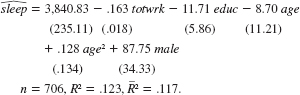
The variable sleep is total minutes per week spent sleeping at night, totwrk is total weekly minutes spent working, educ and age are measured in years, and male is a gender dummy.
(i) All other factors being equal, is there evidence that men sleep more than women How strong is the evidence
(ii) Is there a statistically significant tradeoff between working and sleeping What is the estimated tradeoff
(iii) What other regression do you need to run to test the null hypothesis that, holding other factors fixed, age has no effect on sleeping
Question
Let d be a dummy (binary) variable and let z be a quantitative variable. Consider the model ![Let d be a dummy (binary) variable and let z be a quantitative variable. Consider the model this is a general version of a model with an interaction between a dummy variable and a quantitative variable. [An example is in equation. (i) Since it changes nothing important, set the error to zero, u = 0. Then, when d _ 0 we can write the relationship between y and z as the function f 0 (z) = 0 + 1 z. Write the same relationship when d = 1, where you should use f 1 (z) on the left-hand side to denote the linear function of z. (ii) Assuming that 1 0 (which means the two lines are not parallel), show that the value of z* such that f 0 (z*) = f 1 (z*) is z* = 0 / 1. This is the point at which the two lines intersect [as in Figure 7.2(b)]. Argue that z* is positive if and only if 0 and 1 have opposite signs (iii) Using the data in TWOYEAR.RAW, the following equation can be estimated: where all coefficients and standard errors have been rounded to three decimal places. Using this equation, find the value of totcoll such that the predicted values of log(wage) are the same for men and women. (iv) Based on the equation in part (iii), can women realistically get enough years of college so that their earnings catch up to those of men Explain. Equation Figure Graphs of equation: (a) 0 0, 1 0; (b) 0 0, 1 0. <div style=padding-top: 35px>](https://d2lvgg3v3hfg70.cloudfront.net/SM2712/11eb9ee2_f0ba_713d_8edd_45e69b4a7c56_SM2712_00.jpg)
this is a general version of a model with an interaction between a dummy variable and a quantitative variable. [An example is in equation.
(i) Since it changes nothing important, set the error to zero, u = 0. Then, when d _ 0 we can write the relationship between y and z as the function f 0 (z) = 0 + 1 z. Write the same relationship when d = 1, where you should use f 1 (z) on the left-hand side to denote the linear function of z.
(ii) Assuming that 1 0 (which means the two lines are not parallel), show that the value of z* such that f 0 (z*) = f 1 (z*) is z* = 0 / 1. This is the point at which the two lines intersect [as in Figure 7.2(b)]. Argue that z* is positive if and only if 0 and 1 have opposite signs
(iii) Using the data in TWOYEAR.RAW, the following equation can be estimated:![Let d be a dummy (binary) variable and let z be a quantitative variable. Consider the model this is a general version of a model with an interaction between a dummy variable and a quantitative variable. [An example is in equation. (i) Since it changes nothing important, set the error to zero, u = 0. Then, when d _ 0 we can write the relationship between y and z as the function f 0 (z) = 0 + 1 z. Write the same relationship when d = 1, where you should use f 1 (z) on the left-hand side to denote the linear function of z. (ii) Assuming that 1 0 (which means the two lines are not parallel), show that the value of z* such that f 0 (z*) = f 1 (z*) is z* = 0 / 1. This is the point at which the two lines intersect [as in Figure 7.2(b)]. Argue that z* is positive if and only if 0 and 1 have opposite signs (iii) Using the data in TWOYEAR.RAW, the following equation can be estimated: where all coefficients and standard errors have been rounded to three decimal places. Using this equation, find the value of totcoll such that the predicted values of log(wage) are the same for men and women. (iv) Based on the equation in part (iii), can women realistically get enough years of college so that their earnings catch up to those of men Explain. Equation Figure Graphs of equation: (a) 0 0, 1 0; (b) 0 0, 1 0. <div style=padding-top: 35px>](https://d2lvgg3v3hfg70.cloudfront.net/SM2712/11eb9ee2_f0ba_713e_8edd_891f247b3501_SM2712_00.jpg)
where all coefficients and standard errors have been rounded to three decimal places. Using this equation, find the value of totcoll such that the predicted values of log(wage) are the same for men and women.
(iv) Based on the equation in part (iii), can women realistically get enough years of college so that their earnings catch up to those of men Explain.
Equation![Let d be a dummy (binary) variable and let z be a quantitative variable. Consider the model this is a general version of a model with an interaction between a dummy variable and a quantitative variable. [An example is in equation. (i) Since it changes nothing important, set the error to zero, u = 0. Then, when d _ 0 we can write the relationship between y and z as the function f 0 (z) = 0 + 1 z. Write the same relationship when d = 1, where you should use f 1 (z) on the left-hand side to denote the linear function of z. (ii) Assuming that 1 0 (which means the two lines are not parallel), show that the value of z* such that f 0 (z*) = f 1 (z*) is z* = 0 / 1. This is the point at which the two lines intersect [as in Figure 7.2(b)]. Argue that z* is positive if and only if 0 and 1 have opposite signs (iii) Using the data in TWOYEAR.RAW, the following equation can be estimated: where all coefficients and standard errors have been rounded to three decimal places. Using this equation, find the value of totcoll such that the predicted values of log(wage) are the same for men and women. (iv) Based on the equation in part (iii), can women realistically get enough years of college so that their earnings catch up to those of men Explain. Equation Figure Graphs of equation: (a) 0 0, 1 0; (b) 0 0, 1 0. <div style=padding-top: 35px>](https://d2lvgg3v3hfg70.cloudfront.net/SM2712/11eb9ee2_f0ba_713f_8edd_b3b9093866d4_SM2712_00.jpg)
Figure Graphs of equation: (a) 0 0, 1 0; (b) 0 0, 1 0.![Let d be a dummy (binary) variable and let z be a quantitative variable. Consider the model this is a general version of a model with an interaction between a dummy variable and a quantitative variable. [An example is in equation. (i) Since it changes nothing important, set the error to zero, u = 0. Then, when d _ 0 we can write the relationship between y and z as the function f 0 (z) = 0 + 1 z. Write the same relationship when d = 1, where you should use f 1 (z) on the left-hand side to denote the linear function of z. (ii) Assuming that 1 0 (which means the two lines are not parallel), show that the value of z* such that f 0 (z*) = f 1 (z*) is z* = 0 / 1. This is the point at which the two lines intersect [as in Figure 7.2(b)]. Argue that z* is positive if and only if 0 and 1 have opposite signs (iii) Using the data in TWOYEAR.RAW, the following equation can be estimated: where all coefficients and standard errors have been rounded to three decimal places. Using this equation, find the value of totcoll such that the predicted values of log(wage) are the same for men and women. (iv) Based on the equation in part (iii), can women realistically get enough years of college so that their earnings catch up to those of men Explain. Equation Figure Graphs of equation: (a) 0 0, 1 0; (b) 0 0, 1 0. <div style=padding-top: 35px>](https://d2lvgg3v3hfg70.cloudfront.net/SM2712/11eb9ee2_f0ba_9850_8edd_0504a771f361_SM2712_00.jpg)
this is a general version of a model with an interaction between a dummy variable and a quantitative variable. [An example is in equation.
(i) Since it changes nothing important, set the error to zero, u = 0. Then, when d _ 0 we can write the relationship between y and z as the function f 0 (z) = 0 + 1 z. Write the same relationship when d = 1, where you should use f 1 (z) on the left-hand side to denote the linear function of z.
(ii) Assuming that 1 0 (which means the two lines are not parallel), show that the value of z* such that f 0 (z*) = f 1 (z*) is z* = 0 / 1. This is the point at which the two lines intersect [as in Figure 7.2(b)]. Argue that z* is positive if and only if 0 and 1 have opposite signs
(iii) Using the data in TWOYEAR.RAW, the following equation can be estimated:
where all coefficients and standard errors have been rounded to three decimal places. Using this equation, find the value of totcoll such that the predicted values of log(wage) are the same for men and women.
(iv) Based on the equation in part (iii), can women realistically get enough years of college so that their earnings catch up to those of men Explain.
Equation
Figure Graphs of equation: (a) 0 0, 1 0; (b) 0 0, 1 0.
Question
Use the data in WAGE2.RAW for this exercise.
(i) Estimate the model
and report the results in the usual form. Holding other factors fixed, what is the approximate difference in monthly salary between blacks and nonblacks Is this difference statistically significant
(ii) Add the variables exper 2 and tenure 2 to the equation and show that they are jointly insignificant at even the 20% level.
(iii) Extend the original model to allow the return to education to depend on race and test whether the return to education does depend on race.
(iv) Again, start with the original model, but now allow wages to differ across four groups of people: married and black, married and nonblack, single and black, and single and nonblack. What is the estimated wage differential between married blacks and married nonblacks
Question
Question
The following equations were estimated using the data in BWGHT.RAW: 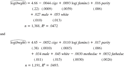
The variables are defined as in Example 4.9, but we have added a dummy variable for whether the child is male and a dummy variable indicating whether the child is classified as white.
(i) In the first equation, interpret the coefficient on the variable cigs. In particular, what is the effect on birth weight from smoking 10 more cigarettes per day
(ii) How much more is a white child predicted to weigh than a nonwhite child, holding the other factors in the first equation fixed Is the difference statistically significant
(iii) Comment on the estimated effect and statistical significance of motheduc.
(iv) From the given information, why are you unable to compute the F statistic for joint significance of motheduc and fatheduc What would you have to do to compute the F statistic
Question
Question
A model that allows major league baseball player salary to differ by position is 
where outfield is the base group.
(i) State the null hypothesis that, controlling for other factors, catchers and outfielders earn, on average, the same amount. Test this hypothesis using the data in MLB1.RAW and comment on the size of the estimated salary differential.
(ii) State and test the null hypothesis that there is no difference in average salary across positions, once other factors have been controlled for.
(iii) Are the results from parts (i) and (ii) consistent If not, explain what is happening.
Question
Use the data in 401KSUBS.RAW for this exercise.
(i) Compute the average, standard deviation, minimum, and maximum values of nettfa in the sample.
(ii) Test the hypothesis that average nettfa does not differ by 401(k) eligibility status; use a two-sided alternative. What is the dollar amount of the estimated difference
(iii) From part (ii) of Computer Exercise, it is clear that e401k is not exogenous in a simple regression model; at a minimum, it changes by income and age. Estimate a multiple linear regression model for nettfa that includes income, age, and e401k as explanatory variables. The income and age variables should appear as quadratics. Now, what is the estimated dollar effect of 401(k) eligibility
(iv) To the model estimated in part (iii), add the interactions e401k • (age _ 41) and e401k • (age _ 41) 2. Note that the average age in the sample is about 41, so that in the new model, the coefficient on e401k is the estimated effect of 401(k) eligibilityat the average age. Which interaction term is significant
(v) Comparing the estimates from parts (iii) and (iv), do the estimated effects of 401(k) eligibility at age 41 differ much Explain.
(vi) Now, drop the interaction terms from the model, but define five family size dummy variables: fsize1, fsize2, fsize3, fsize4, and fsize5. The variable fsize5 is unity for families with five or more members. Include the family size dummies in the model estimated from part (iii); be sure to choose a base group. Are the family dummies significant at the 1% level
(vii) Now, do a Chow test for the model
across the five family size categories, allowing for intercept differences. The restricted sum of squared residuals, SSR r , is obtained from part (vi) because that regression assumes all slopes are the same. The unrestricted sum of squared residuals is SSR ur = SSR 1 = SSR 2 =... = SSR 5 , where SSR f is the sum of squared residuals for the equation estimated using only family size f. You should convince yourself that there are 30 parameters in the unrestricted model (5 intercepts plus 25 slopes) and 10 parameters in the restricted model (5 intercepts plus 5 slopes). Therefore, the number of restrictions being tested is q = 20, and the df for the unrestricted model is 9,275 _ 30 = 9,245.
Exercise There has been much interest in whether the presence of 401(k) pension plans, available to many U.S. workers, increases net savings. The data set 401KSUBS.RAW contains information on net financial assets (nettfa), family income (inc), a binary variable for eligibility in a 401(k) plan (e401k), and several other variables.
(i) What fraction of the families in the sample are eligible for participation in a 401(k) plan
(ii) Estimate a linear probability model explaining 401(k) eligibility in terms of income, age, and gender. Include income and age in quadratic form, and report the results in the usual form.
(iii) Would you say that 401(k) eligibility is independent of income and age What about gender Explain.
(iv) Obtain the fitted values from the linear probability model estimated in part (ii). Are any fitted values negative or greater than one
(v) Using the fitted values from part (iv), define
 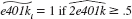 and
and 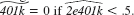 Out of 9,275 families, how many are predicted to be eligible for a 401(k) plan
(vi) For the 5,638 families not eligible for a 401(k), what percentage of these are predicted not to have a 401(k), using the predictor For the 3,637 families eligible for a 401(k) plan, what percentage are predicted to have one (It is helpful if your econometrics package has a "tabulate" command.)
(vii) The overall percent correctly predicted is about 64.9%. Do you think this is a complete description of how well the model does, given your answers in part (vi)
(viii) Add the variable pira as an explanatory variable to the linear probability model. Other things equal, if a family has someone with an individual retirement account, how much higher is the estimated probability that the family is eligible for a 401(k) plan Is it statistically different from zero at the 10% level
(i) Compute the average, standard deviation, minimum, and maximum values of nettfa in the sample.
(ii) Test the hypothesis that average nettfa does not differ by 401(k) eligibility status; use a two-sided alternative. What is the dollar amount of the estimated difference
(iii) From part (ii) of Computer Exercise, it is clear that e401k is not exogenous in a simple regression model; at a minimum, it changes by income and age. Estimate a multiple linear regression model for nettfa that includes income, age, and e401k as explanatory variables. The income and age variables should appear as quadratics. Now, what is the estimated dollar effect of 401(k) eligibility
(iv) To the model estimated in part (iii), add the interactions e401k • (age _ 41) and e401k • (age _ 41) 2. Note that the average age in the sample is about 41, so that in the new model, the coefficient on e401k is the estimated effect of 401(k) eligibilityat the average age. Which interaction term is significant
(v) Comparing the estimates from parts (iii) and (iv), do the estimated effects of 401(k) eligibility at age 41 differ much Explain.
(vi) Now, drop the interaction terms from the model, but define five family size dummy variables: fsize1, fsize2, fsize3, fsize4, and fsize5. The variable fsize5 is unity for families with five or more members. Include the family size dummies in the model estimated from part (iii); be sure to choose a base group. Are the family dummies significant at the 1% level
(vii) Now, do a Chow test for the model
across the five family size categories, allowing for intercept differences. The restricted sum of squared residuals, SSR r , is obtained from part (vi) because that regression assumes all slopes are the same. The unrestricted sum of squared residuals is SSR ur = SSR 1 = SSR 2 =... = SSR 5 , where SSR f is the sum of squared residuals for the equation estimated using only family size f. You should convince yourself that there are 30 parameters in the unrestricted model (5 intercepts plus 25 slopes) and 10 parameters in the restricted model (5 intercepts plus 5 slopes). Therefore, the number of restrictions being tested is q = 20, and the df for the unrestricted model is 9,275 _ 30 = 9,245.
Exercise There has been much interest in whether the presence of 401(k) pension plans, available to many U.S. workers, increases net savings. The data set 401KSUBS.RAW contains information on net financial assets (nettfa), family income (inc), a binary variable for eligibility in a 401(k) plan (e401k), and several other variables.
(i) What fraction of the families in the sample are eligible for participation in a 401(k) plan
(ii) Estimate a linear probability model explaining 401(k) eligibility in terms of income, age, and gender. Include income and age in quadratic form, and report the results in the usual form.
(iii) Would you say that 401(k) eligibility is independent of income and age What about gender Explain.
(iv) Obtain the fitted values from the linear probability model estimated in part (ii). Are any fitted values negative or greater than one
(v) Using the fitted values
from part (iv), define and Out of 9,275 families, how many are predicted to be eligible for a 401(k) plan (vi) For the 5,638 families not eligible for a 401(k), what percentage of these are predicted not to have a 401(k), using the predictor
For the 3,637 families eligible for a 401(k) plan, what percentage are predicted to have one (It is helpful if your econometrics package has a "tabulate" command.)(vii) The overall percent correctly predicted is about 64.9%. Do you think this is a complete description of how well the model does, given your answers in part (vi)
(viii) Add the variable pira as an explanatory variable to the linear probability model. Other things equal, if a family has someone with an individual retirement account, how much higher is the estimated probability that the family is eligible for a 401(k) plan Is it statistically different from zero at the 10% level
Question
Using the data in GPA2.RAW, the following equation was estimated: 
The variable sat is the combined SAT score, hsize is size of the student's high school graduating class, in hundreds, female is a gender dummy variable, and black is a race dummy variable equal to one for blacks and zero otherwise.
(i) Is there strong evidence that hsize 2 should be included in the model From this equation, what is the optimal high school size
(ii) Holding hsize fixed, what is the estimated difference in SAT score between nonblack females and nonblack males How statistically significant is this estimated difference
(iii) What is the estimated difference in SAT score between nonblack males and black males Test the null hypothesis that there is no difference between their scores, against the alternative that there is a difference.
(iv) What is the estimated difference in SAT score between black females and nonblack females What would you need to do to test whether the difference is statistically significant
Question
Use the data set in BEAUTY.RAW, which contains a subset of the variables (but more usable observations than in the regressions) reported by Hamermesh and Biddle (1994).
(i) Find the separate fractions of men and women that are classified as having above average looks. Are more people rated as having above average or below average looks
(ii) Test the null hypothesis that the population fractions of above-average-looking women and men are the same. Report the one-sided p -value that the fraction is higher for women. ( Hint: Estimating a simple linear probability model is easiest.)
(iii) Now estimate the model
separately for men and women, and report the results in the usual form. In both cases, interpret the coefficient on belavg. Explain in words what the hypothesis H 0 : against H 1 :
  means, and find the p -values for men and women.
(iv) Is there convincing evidence that women with above average looks earn more than women with average looks Explain.
(v) For both men and women, add the explanatory variables educ , exper , exper 2 , union , goodhlth , black , married , south , bigcity , smllcity , and service. Do the effects of the "looks" variables change in important ways
(vi) Use the SSR form of the Chow F statistic to test whether the slopes of the regression functions in part (v) differ across men and women. Be sure to allow for an intercept shift under the null.
(i) Find the separate fractions of men and women that are classified as having above average looks. Are more people rated as having above average or below average looks
(ii) Test the null hypothesis that the population fractions of above-average-looking women and men are the same. Report the one-sided p -value that the fraction is higher for women. ( Hint: Estimating a simple linear probability model is easiest.)
(iii) Now estimate the model
separately for men and women, and report the results in the usual form. In both cases, interpret the coefficient on belavg. Explain in words what the hypothesis H 0 :
against H 1 : means, and find the p -values for men and women.(iv) Is there convincing evidence that women with above average looks earn more than women with average looks Explain.
(v) For both men and women, add the explanatory variables educ , exper , exper 2 , union , goodhlth , black , married , south , bigcity , smllcity , and service. Do the effects of the "looks" variables change in important ways
(vi) Use the SSR form of the Chow F statistic to test whether the slopes of the regression functions in part (v) differ across men and women. Be sure to allow for an intercept shift under the null.
Question
Use the data in GPA2.RAW for this exercise.
(i) Consider the equation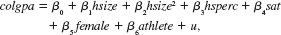
where colgpa is cumulative college grade point average, hsize is size of high school graduating class, in hundreds, hsperc is academic percentile in graduating class, sat is combined SAT score, female is a binary gender variable, and athlete is a binary variable, which is one for tudent-athletes. What are your expectations for the coefficients in this equation Which ones are you unsure about
(ii) Estimate the equation in part (i) and report the results in the usual form. What is the estimated GPA differential between athletes and nonathletes Is it statistically significant
(iii) Drop sat from the model and reestimate the equation. Now, what is the estimated effect of being an athlete Discuss why the estimate is different than that obtained in part (ii).
(iv) In the model from part (i), allow the effect of being an athlete to differ by gender and test the null hypothesis that there is no ceteris paribus difference between women athletes and women nonathletes.
(v) Does the effect of sat on colgpa differ by gender Justify your answer.
Question
Use the data in APPLE.RAW to answer this question.
(i) Define a binary variable as ecobuy _ 1 if ecolbs 0 and ecobuy = 0 if ecolbs = 0. In other words, ecobuy indicates whether, at the prices given, a family would buy any ecologically friendly apples. What fraction of families claim they would buy ecolabeled apples
(ii) Estimate the linear probability model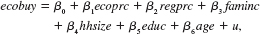 and report the results in the usual form. Carefully interpret the coefficients on the price variables.
(iii) Are the nonprice variables jointly significant in the LPM (Use the usual F statistic, even though it is not valid when there is heteroskedasticity.) Which explanatory variable other than the price variables seems to have the most important effect on the decision to buy ecolabeled apples Does this make sense to you
(iv) In the model from part (ii), replace faminc with log(faminc). Which model fits the data better, using faminc or log(faminc) Interpret the coefficient on log(faminc).
(v) In the estimation in part (iv), how many estimated probabilities are negative How many are bigger than one Should you be concerned
(vi) For the estimation in part (iv), compute the percent correctly predicted for each outcome, ecobuy = 0 and ecobuy = 1. Which outcome is best predicted by the model
(i) Define a binary variable as ecobuy _ 1 if ecolbs 0 and ecobuy = 0 if ecolbs = 0. In other words, ecobuy indicates whether, at the prices given, a family would buy any ecologically friendly apples. What fraction of families claim they would buy ecolabeled apples
(ii) Estimate the linear probability model
and report the results in the usual form. Carefully interpret the coefficients on the price variables.(iii) Are the nonprice variables jointly significant in the LPM (Use the usual F statistic, even though it is not valid when there is heteroskedasticity.) Which explanatory variable other than the price variables seems to have the most important effect on the decision to buy ecolabeled apples Does this make sense to you
(iv) In the model from part (ii), replace faminc with log(faminc). Which model fits the data better, using faminc or log(faminc) Interpret the coefficient on log(faminc).
(v) In the estimation in part (iv), how many estimated probabilities are negative How many are bigger than one Should you be concerned
(vi) For the estimation in part (iv), compute the percent correctly predicted for each outcome, ecobuy = 0 and ecobuy = 1. Which outcome is best predicted by the model
Question
An equation explaining chief executive officer salary is 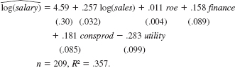
The data used are in CEOSAL1.RAW, where finance, consprod, and utility are binary variables indicating the financial, consumer products, and utilities industries. The omitted industry is transportation.
(i) Compute the approximate percentage difference in estimated salary between the utility and transportation industries, holding sales and roe fixed. Is the difference statistically significant at the 1% level
(ii) Use equation to obtain the exact percentage difference in estimated salary between the utility and transportation industries and compare this with the answer obtained in part (i).
(iii) What is the approximate percentage difference in estimated salary between the consumer products and finance industries Write an equation that would allow you to test whether the difference is statistically significant.
Equation
Question
Question
In Problem, we added the return on the firm's stock, ros, to a model explaining CEO salary; ros turned out to be insignificant. Now, define a dummy variable, rosneg, which is equal to one if ros 0 and equal to zero if ros 0. Use CEOSAL1.RAW to estimate the model 
Discuss the interpretation and statistical significance of
Problem Consider an equation to explain salaries of CEOs in terms of annual firm sales, return on equity (roe, in percentage form), and return on the firm's stock (ros, in percentage form):
(i) In terms of the model parameters, state the null hypothesis that, after controlling for sales and roe, ros has no effect on CEO salary. State the alternative that better stock market performance increases a CEO's salary.
(ii) Using the data in CEOSAL1.RAW, the following equation was obtained by OLS: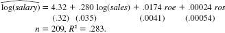
By what percentage is salary predicted to increase if ros increases by 50 points Does ros have a practically large effect on salary
(iii) Test the null hypothesis that ros has no effect on salary against the alternative that ros has a positive effect. Carry out the test at the 10% significance level.
(iv) Would you include ros in a final model explaining CEO compensation in terms of firm performance Explain.
Question
In Example 7.2, let noPC be a dummy variable equal to one if the student does not own a PC, and zero otherwise.
(i) If noPC is used in place of PC in equation, what happens to the intercept in the estimated equation What will be the coefficient on noPC (Hint: Write PC = 1 _ noPC and plug this into the equation
(ii) What will happen to the R-squared if noPC is used in place of PC
(iii) Should PC and noPC both be included as independent variables in the model Explain.
Equation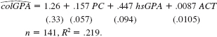
Question
Use the data in SLEEP75.RAW for this exercise. The equation of interest is 
(i) Estimate this equation separately for men and women and report the results in the usual form. Are there notable differences in the two estimated equations
(ii) Compute the Chow test for equality of the parameters in the sleep equation for men and women. Use the form of the test that adds male and the interaction terms male •totwrk, …, male •yngkid and uses the full set of observations. What are the relevant df for the test Should you reject the null at the 5% level
(iii) Now, allow for a different intercept for males and females and determine whether the interaction terms involving male are jointly significant.
(iv) Given the results from parts (ii) and (iii), what would be your final model
Question
To test the effectiveness of a job training program on the subsequent wages of workers, we specify the model 
where train is a binary variable equal to unity if a worker participated in the program. Think of the error term u as containing unobserved worker ability. If less able workers have a greater chance of being selected for the program, and you use an OLS analysis, what can you say about the likely bias in the OLS estimator of 1 (Hint: Refer back to Chapter 3.)
where train is a binary variable equal to unity if a worker participated in the program. Think of the error term u as containing unobserved worker ability. If less able workers have a greater chance of being selected for the program, and you use an OLS analysis, what can you say about the likely bias in the OLS estimator of 1 (Hint: Refer back to Chapter 3.)
Question
Question
In the example in equation, suppose that we define outlf to be one if the woman is out of the labor force, and zero otherwise.
(i) If we regress outlf on all of the independent variables in equation, what will happen to the intercept and slope estimates (Hint: inlf = 1 _ outlf. Plug this into the population equation inlf = 0 + 1 nwifeinc + 2 educ + … and rearrange.)
(ii) What will happen to the standard errors on the intercept and slope estimates
(iii) What will happen to the R-squared
Equation
Question
Use the data in LOANAPP.RAW for this exercise. The binary variable to be explained is approve, which is equal to one if a mortgage loan to an individual was approved. The key explanatory variable is white, a dummy variable equal to one if the applicant was white. The other applicants in the data set are black and Hispanic.
To test for discrimination in the mortgage loan market, a linear probability model can be used:
(i) If there is discrimination against minorities, and the appropriate factors have been controlled for, what is the sign of 1
(ii) Regress approve on white and report the results in the usual form. Interpret the coefficient on white. Is it statistically significant Is it practically large
(iii) As controls, add the variables hrat, obrat, loanprc, unem, male, married, dep, sch, cosign, chist, pubrec, mortlat1, mortlat2, and vr. What happens to the coefficient on white Is there still evidence of discrimination against nonwhites
(iv) Now, allow the effect of race to interact with the variable measuring other obligations as a percentage of income (obrat). Is the interaction term significant
(v) Using the model from part (iv), what is the effect of being white on the probability of approval when obrat = 32, which is roughly the mean value in the sample Obtain a 95% confidence interval for this effect.

Unlock Deck
Sign up to unlock the cards in this deck!
Unlock Deck
Unlock Deck
1/24
Play
Full screen (f)
Deck 7: Multiple Regression Analysis With Qualitative Information: Binary or Dummy Variables
1
Suppose you collect data from a survey on wages, education, experience, and gender. In addition, you ask for information about marijuana usage. The original question is: "On how many separate occasions last month did you smoke marijuana "
(i) Write an equation that would allow you to estimate the effects of marijuana usage on wage, while controlling for other factors. You should be able to make statements such as, "Smoking marijuana five more times per month is estimated to change wage by x%."
(ii) Write a model that would allow you to test whether drug usage has different effects on wages for men and women. How would you test that there are no differences in the effects of drug usage for men and women
(iii) Suppose you think it is better to measure marijuana usage by putting people into one of four categories: nonuser, light user (1 to 5 times per month), moderate user (6 to 10 times per month), and heavy user (more than 10 times per month). Now, write a model that allows you to estimate the effects of marijuana usage on wage.
(iv) Using the model in part (iii), explain in detail how to test the null hypothesis that marijuana usage has no effect on wage. Be very specific and include a careful listing of degrees of freedom.
(v) What are some potential problems with drawing causal inference using the survey data that you collected
(i)
Consider the model that relates wages to education, experience, and gender and marijuana usage given by: Where,
  Wage-rate
  The number of marijuana used by the employee per month
  The education level of the employee
  The experience level of the employee
  The binary variable which is equal to 1 for Male
From this wage-equation, one could infer that if increases by 1 time per month, the wage would change by
  , other factors being controlled for
When the increases by 5 more times per month, the wage would change by
  .
.
Here .
.
(ii)
In order to test whether drug usage has different effects on wages for men and women, the interaction term would be added to the model, such that the model becomes:
  Now, test for the significance of the coefficient
  using Wald test such that:
  The t-statistics is computed as:
  If the t-statistic as obtained is greater than the critical t-statistic at n-6 degree of freedom, where n is the number of observations, it is concluded that there is statistically significant difference in the effects that the drug usage has on wages for men and women.
(iii)
When the four categories of people making marijuana usage is considered:
1) Nonuse
2) Light user (1 to 5 times per month)
3) Moderate user (6 to 10 times per month)
4) Heavy user (more than 10 times per month)
The model becomes: Where,
  The binary variable for light user
  The binary variable for Moderate user
  The binary variable for Heavy user
Consider that the binary variable for non-user is kept as base.
(iv)
Using the model: In order to test for the null hypothesis that marijuana usage has no effect on wage, the test proceedings are as follows:
  Conduct a Wald test with such specifications.
It shall be noted that, there are 3 restrictions in the given model and that there are 8 coefficients
So conduct F-test with the degree of freedom in the numerator=3 and degree of freedom in the denominator=n-8.
(v)
Some of the potential problems with drawing causal inference using the survey data which has been collected includes problems relating to omitted variable bias, such that the error term becomes correlated with some of the explanatory variables in the model, thereby leading to biasedness of the coefficients estimated using OLS method
Such omitted variables could be societal status of the employee which is directly related to marijuana usage, in addition to employees' ability and motivation that directly affect wage earned by the employee.
Consider the model that relates wages to education, experience, and gender and marijuana usage given by:
Where, Wage-rate The number of marijuana used by the employee per month The education level of the employee The experience level of the employee The binary variable which is equal to 1 for MaleFrom this wage-equation, one could infer that if
increases by 1 time per month, the wage would change by , other factors being controlled forWhen the
increases by 5 more times per month, the wage would change by .Here
.(ii)
In order to test whether drug usage has different effects on wages for men and women, the interaction term
would be added to the model, such that the model becomes: Now, test for the significance of the coefficient using Wald test such that: The t-statistics is computed as: If the t-statistic as obtained is greater than the critical t-statistic at n-6 degree of freedom, where n is the number of observations, it is concluded that there is statistically significant difference in the effects that the drug usage has on wages for men and women.(iii)
When the four categories of people making marijuana usage is considered:
1) Nonuse
2) Light user (1 to 5 times per month)
3) Moderate user (6 to 10 times per month)
4) Heavy user (more than 10 times per month)
The model becomes:
Where, The binary variable for light user The binary variable for Moderate user The binary variable for Heavy userConsider that the binary variable for non-user is kept as base.
(iv)
Using the model:
In order to test for the null hypothesis that marijuana usage has no effect on wage, the test proceedings are as follows: Conduct a Wald test with such specifications.It shall be noted that, there are 3 restrictions in the given model and that there are 8 coefficients
So conduct F-test with the degree of freedom in the numerator=3 and degree of freedom in the denominator=n-8.
(v)
Some of the potential problems with drawing causal inference using the survey data which has been collected includes problems relating to omitted variable bias, such that the error term becomes correlated with some of the explanatory variables in the model, thereby leading to biasedness of the coefficients estimated using OLS method
Such omitted variables could be societal status of the employee which is directly related to marijuana usage, in addition to employees' ability and motivation that directly affect wage earned by the employee.
2
Use the data in GPA1.RAW for this exercise.
(i) Add the variables mothcoll and fathcoll to the equation estimated in (7.6) and report the results in the usual form. What happens to the estimated effect of PC ownership Is PC still statistically significant
(ii) Test for joint significance of mothcoll and fathcoll in the equation from part (i) and be sure to report the p-value.
(iii) Add hsGPA 2 to the model from part (i) and decide whether this generalization is needed.
Consider the data GPA1.RAW to solve the subparts.
(i)
Then multiple linear regression model including all the four explanatory variables is given as: Where, the intercept
  is the predicted value of
  when the entire
  are equal to zero and
  are the slope coefficient. To do the regression analysis adds the variables and the variables mothcoll and fathcoll in the regression equation 7.6 of the text book.
The procedure to do the regression analysis is given as below:
1. Click on the "Stat option Regression Regression", a new dialog box will open, select the "colGPA" as response variable and the "PC, hsGPA, ACT, mothcoll and fathcoll" as the predictors then press "OK" button. The screen shot is shown below: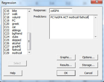 2. Press "OK" option in the above dialog box, the screenshot of the obtained output is shown below:
 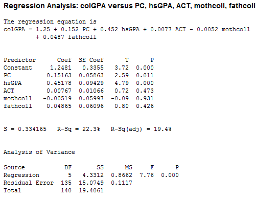 The usual form of the obtained regression model is as below:
  The estimated effect of PC ownership is given by the coefficient of
  , which is 0.1512. Thus, the coefficient of PC is positive so it depicts that the colGPA is expected to increase (or decreases) by 0.152 percentages as PC increases (or decreases) by 1. The p -value of the coefficient of
  is 0.01 which is less than the level of significance p -value (0.05). Hence, at 5% level of significance the variable
  is still statistically significant asin equation 7.6.
(ii)
On testing for the joint significance of the variables mothcoll and fathcoll using the Wald test.
The result is shown below: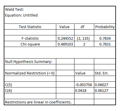 The p -value of F-statistic is 0.7834 which is greater than the critical p-value of 0.05 at 5% level of significance, indicating that the variables mothcoll and fathcoll are jointly insignificant at 5% level of significance.
(iii)
To add the variable Click on the calculator, a new dialog box will appear then store results in variable hsGPASQ and then write the expression as shown below:
 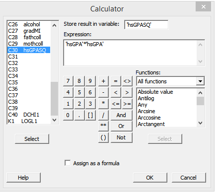 2. Now press OK tab in the above dialog box. The variable hsGPASQ will be created. Now follow the same procedure as done in part (a) and add the variable hsGPASQ in the predators. The screenshot of the result obtained is shown below:
 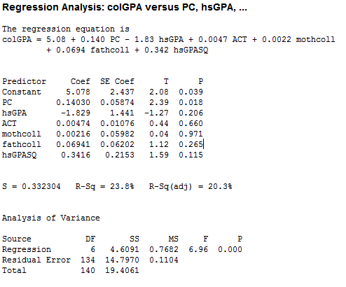 The p -value of the coefficient of
  is 0.115 which is greater than the critical p -value of 0.05 at 5% level of significance, indicating that the generalization by adding
  is not needed.
(i)
Then multiple linear regression model including all the four explanatory variables is given as:
Where, the intercept is the predicted value of when the entire are equal to zero and are the slope coefficient. To do the regression analysis adds the variables and the variables mothcoll and fathcoll in the regression equation 7.6 of the text book. The procedure to do the regression analysis is given as below:
1. Click on the "Stat option Regression Regression", a new dialog box will open, select the "colGPA" as response variable and the "PC, hsGPA, ACT, mothcoll and fathcoll" as the predictors then press "OK" button. The screen shot is shown below:
2. Press "OK" option in the above dialog box, the screenshot of the obtained output is shown below: The usual form of the obtained regression model is as below: The estimated effect of PC ownership is given by the coefficient of , which is 0.1512. Thus, the coefficient of PC is positive so it depicts that the colGPA is expected to increase (or decreases) by 0.152 percentages as PC increases (or decreases) by 1. The p -value of the coefficient of is 0.01 which is less than the level of significance p -value (0.05). Hence, at 5% level of significance the variable is still statistically significant asin equation 7.6.(ii)
On testing for the joint significance of the variables mothcoll and fathcoll using the Wald test.
The result is shown below:
The p -value of F-statistic is 0.7834 which is greater than the critical p-value of 0.05 at 5% level of significance, indicating that the variables mothcoll and fathcoll are jointly insignificant at 5% level of significance.(iii)
To add the variable
Click on the calculator, a new dialog box will appear then store results in variable hsGPASQ and then write the expression as shown below: 2. Now press OK tab in the above dialog box. The variable hsGPASQ will be created. Now follow the same procedure as done in part (a) and add the variable hsGPASQ in the predators. The screenshot of the result obtained is shown below: The p -value of the coefficient of is 0.115 which is greater than the critical p -value of 0.05 at 5% level of significance, indicating that the generalization by adding is not needed. 3
There has been much interest in whether the presence of 401(k) pension plans, available to many U.S. workers, increases net savings. The data set 401KSUBS.RAW contains information on net financial assets (nettfa), family income (inc), a binary variable for eligibility in a 401(k) plan (e401k), and several other variables.
(i) What fraction of the families in the sample are eligible for participation in a 401(k) plan
(ii) Estimate a linear probability model explaining 401(k) eligibility in terms of income, age, and gender. Include income and age in quadratic form, and report the results in the usual form.
(iii) Would you say that 401(k) eligibility is independent of income and age What about gender Explain.
(iv) Obtain the fitted values from the linear probability model estimated in part (ii). Are any fitted values negative or greater than one
(v) Using the fitted values from part (iv), define and Out of 9,275 families, how many are predicted to be eligible for a 401(k) plan
(vi) For the 5,638 families not eligible for a 401(k), what percentage of these are predicted not to have a 401(k), using the predictor For the 3,637 families eligible for a 401(k) plan, what percentage are predicted to have one (It is helpful if your econometrics package has a "tabulate" command.)
(vii) The overall percent correctly predicted is about 64.9%. Do you think this is a complete description of how well the model does, given your answers in part (vi)
(viii) Add the variable pira as an explanatory variable to the linear probability model. Other things equal, if a family has someone with an individual retirement account, how much higher is the estimated probability that the family is eligible for a 401(k) plan Is it statistically different from zero at the 10% level
(i) What fraction of the families in the sample are eligible for participation in a 401(k) plan
(ii) Estimate a linear probability model explaining 401(k) eligibility in terms of income, age, and gender. Include income and age in quadratic form, and report the results in the usual form.
(iii) Would you say that 401(k) eligibility is independent of income and age What about gender Explain.
(iv) Obtain the fitted values from the linear probability model estimated in part (ii). Are any fitted values negative or greater than one
(v) Using the fitted values
from part (iv), define and Out of 9,275 families, how many are predicted to be eligible for a 401(k) plan (vi) For the 5,638 families not eligible for a 401(k), what percentage of these are predicted not to have a 401(k), using the predictor
For the 3,637 families eligible for a 401(k) plan, what percentage are predicted to have one (It is helpful if your econometrics package has a "tabulate" command.)(vii) The overall percent correctly predicted is about 64.9%. Do you think this is a complete description of how well the model does, given your answers in part (vi)
(viii) Add the variable pira as an explanatory variable to the linear probability model. Other things equal, if a family has someone with an individual retirement account, how much higher is the estimated probability that the family is eligible for a 401(k) plan Is it statistically different from zero at the 10% level
NO ANSWER
4
Using the data in SLEEP75.RAW (see also Problem), we obtain the estimated equation
The variable sleep is total minutes per week spent sleeping at night, totwrk is total weekly minutes spent working, educ and age are measured in years, and male is a gender dummy.
(i) All other factors being equal, is there evidence that men sleep more than women How strong is the evidence
(ii) Is there a statistically significant tradeoff between working and sleeping What is the estimated tradeoff
(iii) What other regression do you need to run to test the null hypothesis that, holding other factors fixed, age has no effect on sleeping
Unlock Deck
Unlock for access to all 24 flashcards in this deck.
Unlock Deck
k this deck
5
Let d be a dummy (binary) variable and let z be a quantitative variable. Consider the model
this is a general version of a model with an interaction between a dummy variable and a quantitative variable. [An example is in equation.
(i) Since it changes nothing important, set the error to zero, u = 0. Then, when d _ 0 we can write the relationship between y and z as the function f 0 (z) = 0 + 1 z. Write the same relationship when d = 1, where you should use f 1 (z) on the left-hand side to denote the linear function of z.
(ii) Assuming that 1 0 (which means the two lines are not parallel), show that the value of z* such that f 0 (z*) = f 1 (z*) is z* = 0 / 1. This is the point at which the two lines intersect [as in Figure 7.2(b)]. Argue that z* is positive if and only if 0 and 1 have opposite signs
(iii) Using the data in TWOYEAR.RAW, the following equation can be estimated:
where all coefficients and standard errors have been rounded to three decimal places. Using this equation, find the value of totcoll such that the predicted values of log(wage) are the same for men and women.
(iv) Based on the equation in part (iii), can women realistically get enough years of college so that their earnings catch up to those of men Explain.
Equation
Figure Graphs of equation: (a) 0 0, 1 0; (b) 0 0, 1 0.
Unlock Deck
Unlock for access to all 24 flashcards in this deck.
Unlock Deck
k this deck
6
Use the data in WAGE2.RAW for this exercise.
(i) Estimate the model
and report the results in the usual form. Holding other factors fixed, what is the approximate difference in monthly salary between blacks and nonblacks Is this difference statistically significant
(ii) Add the variables exper 2 and tenure 2 to the equation and show that they are jointly insignificant at even the 20% level.
(iii) Extend the original model to allow the return to education to depend on race and test whether the return to education does depend on race.
(iv) Again, start with the original model, but now allow wages to differ across four groups of people: married and black, married and nonblack, single and black, and single and nonblack. What is the estimated wage differential between married blacks and married nonblacks
(i) Estimate the model
and report the results in the usual form. Holding other factors fixed, what is the approximate difference in monthly salary between blacks and nonblacks Is this difference statistically significant
(ii) Add the variables exper 2 and tenure 2 to the equation and show that they are jointly insignificant at even the 20% level.
(iii) Extend the original model to allow the return to education to depend on race and test whether the return to education does depend on race.
(iv) Again, start with the original model, but now allow wages to differ across four groups of people: married and black, married and nonblack, single and black, and single and nonblack. What is the estimated wage differential between married blacks and married nonblacks
Unlock Deck
Unlock for access to all 24 flashcards in this deck.
Unlock Deck
k this deck
7
Use the data in NBASAL.RAW for this exercise.
(i) Estimate a linear regression model relating points per game to experience in the league and position (guard, forward, or center). Include experience in quadratic form and use centers as the base group. Report the results in the usual form.(ii) Why do you not include all three position dummy variables in part (i)
(iii) Holding experience fixed, does a guard score more than a center How much more Is the difference statistically significant
(iv) Now, add marital status to the equation. Holding position and experience fixed, are married players more productive (based on points per game)
(v) Add interactions of marital status with both experience variables. In this expanded model, is there strong evidence that marital status affects points per game
(vi) Estimate the model from part (iv) but use assists per game as the dependent variable. Are there any notable differences from part (iv) Discuss.
Unlock Deck
Unlock for access to all 24 flashcards in this deck.
Unlock Deck
k this deck
8
The following equations were estimated using the data in BWGHT.RAW:
The variables are defined as in Example 4.9, but we have added a dummy variable for whether the child is male and a dummy variable indicating whether the child is classified as white.
(i) In the first equation, interpret the coefficient on the variable cigs. In particular, what is the effect on birth weight from smoking 10 more cigarettes per day
(ii) How much more is a white child predicted to weigh than a nonwhite child, holding the other factors in the first equation fixed Is the difference statistically significant
(iii) Comment on the estimated effect and statistical significance of motheduc.
(iv) From the given information, why are you unable to compute the F statistic for joint significance of motheduc and fatheduc What would you have to do to compute the F statistic
Unlock Deck
Unlock for access to all 24 flashcards in this deck.
Unlock Deck
k this deck
9
For a child i living in a particular a school district, let voucher i be a dummy variable equal to one if a child is selected to participate in a school voucher program, and let score i be that child's score on a subsequent standardized exam. Suppose that the participation variable, voucher i , is completely randomized in the sense that it is independent of both observed and unobserved factors that can affect the test score.
(i) If you run a simple regression score i on voucher i using a random sample of size n, does the OLS estimator provide an unbiased estimator of the effect of the voucher program
(ii) Suppose you can collect additional background information, such as family income, family structure (e.g., whether the child lives with both parents), and parents' education levels. Do you need to control for these factors to obtain an unbiased estimator of the effects of the voucher program Explain.
(iii) Why should you include the family background variables in the regression Is there a situation in which you would not include the background variables
Unlock Deck
Unlock for access to all 24 flashcards in this deck.
Unlock Deck
k this deck
10
A model that allows major league baseball player salary to differ by position is
where outfield is the base group.
(i) State the null hypothesis that, controlling for other factors, catchers and outfielders earn, on average, the same amount. Test this hypothesis using the data in MLB1.RAW and comment on the size of the estimated salary differential.
(ii) State and test the null hypothesis that there is no difference in average salary across positions, once other factors have been controlled for.
(iii) Are the results from parts (i) and (ii) consistent If not, explain what is happening.
Unlock Deck
Unlock for access to all 24 flashcards in this deck.
Unlock Deck
k this deck
11
Use the data in 401KSUBS.RAW for this exercise.
(i) Compute the average, standard deviation, minimum, and maximum values of nettfa in the sample.
(ii) Test the hypothesis that average nettfa does not differ by 401(k) eligibility status; use a two-sided alternative. What is the dollar amount of the estimated difference
(iii) From part (ii) of Computer Exercise, it is clear that e401k is not exogenous in a simple regression model; at a minimum, it changes by income and age. Estimate a multiple linear regression model for nettfa that includes income, age, and e401k as explanatory variables. The income and age variables should appear as quadratics. Now, what is the estimated dollar effect of 401(k) eligibility
(iv) To the model estimated in part (iii), add the interactions e401k • (age _ 41) and e401k • (age _ 41) 2. Note that the average age in the sample is about 41, so that in the new model, the coefficient on e401k is the estimated effect of 401(k) eligibilityat the average age. Which interaction term is significant
(v) Comparing the estimates from parts (iii) and (iv), do the estimated effects of 401(k) eligibility at age 41 differ much Explain.
(vi) Now, drop the interaction terms from the model, but define five family size dummy variables: fsize1, fsize2, fsize3, fsize4, and fsize5. The variable fsize5 is unity for families with five or more members. Include the family size dummies in the model estimated from part (iii); be sure to choose a base group. Are the family dummies significant at the 1% level
(vii) Now, do a Chow test for the model
across the five family size categories, allowing for intercept differences. The restricted sum of squared residuals, SSR r , is obtained from part (vi) because that regression assumes all slopes are the same. The unrestricted sum of squared residuals is SSR ur = SSR 1 = SSR 2 =... = SSR 5 , where SSR f is the sum of squared residuals for the equation estimated using only family size f. You should convince yourself that there are 30 parameters in the unrestricted model (5 intercepts plus 25 slopes) and 10 parameters in the restricted model (5 intercepts plus 5 slopes). Therefore, the number of restrictions being tested is q = 20, and the df for the unrestricted model is 9,275 _ 30 = 9,245.
Exercise There has been much interest in whether the presence of 401(k) pension plans, available to many U.S. workers, increases net savings. The data set 401KSUBS.RAW contains information on net financial assets (nettfa), family income (inc), a binary variable for eligibility in a 401(k) plan (e401k), and several other variables.
(i) What fraction of the families in the sample are eligible for participation in a 401(k) plan
(ii) Estimate a linear probability model explaining 401(k) eligibility in terms of income, age, and gender. Include income and age in quadratic form, and report the results in the usual form.
(iii) Would you say that 401(k) eligibility is independent of income and age What about gender Explain.
(iv) Obtain the fitted values from the linear probability model estimated in part (ii). Are any fitted values negative or greater than one
(v) Using the fitted values from part (iv), define and Out of 9,275 families, how many are predicted to be eligible for a 401(k) plan
(vi) For the 5,638 families not eligible for a 401(k), what percentage of these are predicted not to have a 401(k), using the predictor For the 3,637 families eligible for a 401(k) plan, what percentage are predicted to have one (It is helpful if your econometrics package has a "tabulate" command.)
(vii) The overall percent correctly predicted is about 64.9%. Do you think this is a complete description of how well the model does, given your answers in part (vi)
(viii) Add the variable pira as an explanatory variable to the linear probability model. Other things equal, if a family has someone with an individual retirement account, how much higher is the estimated probability that the family is eligible for a 401(k) plan Is it statistically different from zero at the 10% level
(i) Compute the average, standard deviation, minimum, and maximum values of nettfa in the sample.
(ii) Test the hypothesis that average nettfa does not differ by 401(k) eligibility status; use a two-sided alternative. What is the dollar amount of the estimated difference
(iii) From part (ii) of Computer Exercise, it is clear that e401k is not exogenous in a simple regression model; at a minimum, it changes by income and age. Estimate a multiple linear regression model for nettfa that includes income, age, and e401k as explanatory variables. The income and age variables should appear as quadratics. Now, what is the estimated dollar effect of 401(k) eligibility
(iv) To the model estimated in part (iii), add the interactions e401k • (age _ 41) and e401k • (age _ 41) 2. Note that the average age in the sample is about 41, so that in the new model, the coefficient on e401k is the estimated effect of 401(k) eligibilityat the average age. Which interaction term is significant
(v) Comparing the estimates from parts (iii) and (iv), do the estimated effects of 401(k) eligibility at age 41 differ much Explain.
(vi) Now, drop the interaction terms from the model, but define five family size dummy variables: fsize1, fsize2, fsize3, fsize4, and fsize5. The variable fsize5 is unity for families with five or more members. Include the family size dummies in the model estimated from part (iii); be sure to choose a base group. Are the family dummies significant at the 1% level
(vii) Now, do a Chow test for the model
across the five family size categories, allowing for intercept differences. The restricted sum of squared residuals, SSR r , is obtained from part (vi) because that regression assumes all slopes are the same. The unrestricted sum of squared residuals is SSR ur = SSR 1 = SSR 2 =... = SSR 5 , where SSR f is the sum of squared residuals for the equation estimated using only family size f. You should convince yourself that there are 30 parameters in the unrestricted model (5 intercepts plus 25 slopes) and 10 parameters in the restricted model (5 intercepts plus 5 slopes). Therefore, the number of restrictions being tested is q = 20, and the df for the unrestricted model is 9,275 _ 30 = 9,245.
Exercise There has been much interest in whether the presence of 401(k) pension plans, available to many U.S. workers, increases net savings. The data set 401KSUBS.RAW contains information on net financial assets (nettfa), family income (inc), a binary variable for eligibility in a 401(k) plan (e401k), and several other variables.
(i) What fraction of the families in the sample are eligible for participation in a 401(k) plan
(ii) Estimate a linear probability model explaining 401(k) eligibility in terms of income, age, and gender. Include income and age in quadratic form, and report the results in the usual form.
(iii) Would you say that 401(k) eligibility is independent of income and age What about gender Explain.
(iv) Obtain the fitted values from the linear probability model estimated in part (ii). Are any fitted values negative or greater than one
(v) Using the fitted values
from part (iv), define and Out of 9,275 families, how many are predicted to be eligible for a 401(k) plan (vi) For the 5,638 families not eligible for a 401(k), what percentage of these are predicted not to have a 401(k), using the predictor
For the 3,637 families eligible for a 401(k) plan, what percentage are predicted to have one (It is helpful if your econometrics package has a "tabulate" command.)(vii) The overall percent correctly predicted is about 64.9%. Do you think this is a complete description of how well the model does, given your answers in part (vi)
(viii) Add the variable pira as an explanatory variable to the linear probability model. Other things equal, if a family has someone with an individual retirement account, how much higher is the estimated probability that the family is eligible for a 401(k) plan Is it statistically different from zero at the 10% level
Unlock Deck
Unlock for access to all 24 flashcards in this deck.
Unlock Deck
k this deck
12
Using the data in GPA2.RAW, the following equation was estimated:
The variable sat is the combined SAT score, hsize is size of the student's high school graduating class, in hundreds, female is a gender dummy variable, and black is a race dummy variable equal to one for blacks and zero otherwise.
(i) Is there strong evidence that hsize 2 should be included in the model From this equation, what is the optimal high school size
(ii) Holding hsize fixed, what is the estimated difference in SAT score between nonblack females and nonblack males How statistically significant is this estimated difference
(iii) What is the estimated difference in SAT score between nonblack males and black males Test the null hypothesis that there is no difference between their scores, against the alternative that there is a difference.
(iv) What is the estimated difference in SAT score between black females and nonblack females What would you need to do to test whether the difference is statistically significant
Unlock Deck
Unlock for access to all 24 flashcards in this deck.
Unlock Deck
k this deck
13
Use the data set in BEAUTY.RAW, which contains a subset of the variables (but more usable observations than in the regressions) reported by Hamermesh and Biddle (1994).
(i) Find the separate fractions of men and women that are classified as having above average looks. Are more people rated as having above average or below average looks
(ii) Test the null hypothesis that the population fractions of above-average-looking women and men are the same. Report the one-sided p -value that the fraction is higher for women. ( Hint: Estimating a simple linear probability model is easiest.)
(iii) Now estimate the model
separately for men and women, and report the results in the usual form. In both cases, interpret the coefficient on belavg. Explain in words what the hypothesis H 0 : against H 1 : means, and find the p -values for men and women.
(iv) Is there convincing evidence that women with above average looks earn more than women with average looks Explain.
(v) For both men and women, add the explanatory variables educ , exper , exper 2 , union , goodhlth , black , married , south , bigcity , smllcity , and service. Do the effects of the "looks" variables change in important ways
(vi) Use the SSR form of the Chow F statistic to test whether the slopes of the regression functions in part (v) differ across men and women. Be sure to allow for an intercept shift under the null.
(i) Find the separate fractions of men and women that are classified as having above average looks. Are more people rated as having above average or below average looks
(ii) Test the null hypothesis that the population fractions of above-average-looking women and men are the same. Report the one-sided p -value that the fraction is higher for women. ( Hint: Estimating a simple linear probability model is easiest.)
(iii) Now estimate the model
separately for men and women, and report the results in the usual form. In both cases, interpret the coefficient on belavg. Explain in words what the hypothesis H 0 :
against H 1 : means, and find the p -values for men and women.(iv) Is there convincing evidence that women with above average looks earn more than women with average looks Explain.
(v) For both men and women, add the explanatory variables educ , exper , exper 2 , union , goodhlth , black , married , south , bigcity , smllcity , and service. Do the effects of the "looks" variables change in important ways
(vi) Use the SSR form of the Chow F statistic to test whether the slopes of the regression functions in part (v) differ across men and women. Be sure to allow for an intercept shift under the null.
Unlock Deck
Unlock for access to all 24 flashcards in this deck.
Unlock Deck
k this deck
14
Use the data in GPA2.RAW for this exercise.
(i) Consider the equation
where colgpa is cumulative college grade point average, hsize is size of high school graduating class, in hundreds, hsperc is academic percentile in graduating class, sat is combined SAT score, female is a binary gender variable, and athlete is a binary variable, which is one for tudent-athletes. What are your expectations for the coefficients in this equation Which ones are you unsure about
(ii) Estimate the equation in part (i) and report the results in the usual form. What is the estimated GPA differential between athletes and nonathletes Is it statistically significant
(iii) Drop sat from the model and reestimate the equation. Now, what is the estimated effect of being an athlete Discuss why the estimate is different than that obtained in part (ii).
(iv) In the model from part (i), allow the effect of being an athlete to differ by gender and test the null hypothesis that there is no ceteris paribus difference between women athletes and women nonathletes.
(v) Does the effect of sat on colgpa differ by gender Justify your answer.
(i) Consider the equation
where colgpa is cumulative college grade point average, hsize is size of high school graduating class, in hundreds, hsperc is academic percentile in graduating class, sat is combined SAT score, female is a binary gender variable, and athlete is a binary variable, which is one for tudent-athletes. What are your expectations for the coefficients in this equation Which ones are you unsure about
(ii) Estimate the equation in part (i) and report the results in the usual form. What is the estimated GPA differential between athletes and nonathletes Is it statistically significant
(iii) Drop sat from the model and reestimate the equation. Now, what is the estimated effect of being an athlete Discuss why the estimate is different than that obtained in part (ii).
(iv) In the model from part (i), allow the effect of being an athlete to differ by gender and test the null hypothesis that there is no ceteris paribus difference between women athletes and women nonathletes.
(v) Does the effect of sat on colgpa differ by gender Justify your answer.
Unlock Deck
Unlock for access to all 24 flashcards in this deck.
Unlock Deck
k this deck
15
Use the data in APPLE.RAW to answer this question.
(i) Define a binary variable as ecobuy _ 1 if ecolbs 0 and ecobuy = 0 if ecolbs = 0. In other words, ecobuy indicates whether, at the prices given, a family would buy any ecologically friendly apples. What fraction of families claim they would buy ecolabeled apples
(ii) Estimate the linear probability model and report the results in the usual form. Carefully interpret the coefficients on the price variables.
(iii) Are the nonprice variables jointly significant in the LPM (Use the usual F statistic, even though it is not valid when there is heteroskedasticity.) Which explanatory variable other than the price variables seems to have the most important effect on the decision to buy ecolabeled apples Does this make sense to you
(iv) In the model from part (ii), replace faminc with log(faminc). Which model fits the data better, using faminc or log(faminc) Interpret the coefficient on log(faminc).
(v) In the estimation in part (iv), how many estimated probabilities are negative How many are bigger than one Should you be concerned
(vi) For the estimation in part (iv), compute the percent correctly predicted for each outcome, ecobuy = 0 and ecobuy = 1. Which outcome is best predicted by the model
(i) Define a binary variable as ecobuy _ 1 if ecolbs 0 and ecobuy = 0 if ecolbs = 0. In other words, ecobuy indicates whether, at the prices given, a family would buy any ecologically friendly apples. What fraction of families claim they would buy ecolabeled apples
(ii) Estimate the linear probability model
and report the results in the usual form. Carefully interpret the coefficients on the price variables.(iii) Are the nonprice variables jointly significant in the LPM (Use the usual F statistic, even though it is not valid when there is heteroskedasticity.) Which explanatory variable other than the price variables seems to have the most important effect on the decision to buy ecolabeled apples Does this make sense to you
(iv) In the model from part (ii), replace faminc with log(faminc). Which model fits the data better, using faminc or log(faminc) Interpret the coefficient on log(faminc).
(v) In the estimation in part (iv), how many estimated probabilities are negative How many are bigger than one Should you be concerned
(vi) For the estimation in part (iv), compute the percent correctly predicted for each outcome, ecobuy = 0 and ecobuy = 1. Which outcome is best predicted by the model
Unlock Deck
Unlock for access to all 24 flashcards in this deck.
Unlock Deck
k this deck
16
An equation explaining chief executive officer salary is
The data used are in CEOSAL1.RAW, where finance, consprod, and utility are binary variables indicating the financial, consumer products, and utilities industries. The omitted industry is transportation.
(i) Compute the approximate percentage difference in estimated salary between the utility and transportation industries, holding sales and roe fixed. Is the difference statistically significant at the 1% level
(ii) Use equation to obtain the exact percentage difference in estimated salary between the utility and transportation industries and compare this with the answer obtained in part (i).
(iii) What is the approximate percentage difference in estimated salary between the consumer products and finance industries Write an equation that would allow you to test whether the difference is statistically significant.
Equation
Unlock Deck
Unlock for access to all 24 flashcards in this deck.
Unlock Deck
k this deck
17
Use the data in CHARITY.RAW to answer this question. The variable respond is a dummy variable equal to one if a person responded with a contribution on the most recent mailing sent by a charitable organization. The variable resplast is a dummy variable equal to one if the person responded to the previous mailing, avggift is the average of past gifts (in Dutch guilders), and propresp is the proportion of times the person has responded to past mailings.
(i) Estimate a linear probability model relating respond to resplast and avggift. Report the results in the usual form, and interpret the coefficient on resplast.
(ii) Does the average value of past gifts seem to affect the probability of responding
(iii) Add the variable propresp to the model, and interpret its coefficient. (Be careful here: an increase of one in propresp is the largest possible change.)
(iv) What happened to the coefficient on resplast when propresp was added to the regression Does this make sense
(v) Add mailsyear, the number of mailings per year, to the model. How big is its estimated effect Why might this not be a good estimate of the causal effect of mailings on responding
Unlock Deck
Unlock for access to all 24 flashcards in this deck.
Unlock Deck
k this deck
18
In Problem, we added the return on the firm's stock, ros, to a model explaining CEO salary; ros turned out to be insignificant. Now, define a dummy variable, rosneg, which is equal to one if ros 0 and equal to zero if ros 0. Use CEOSAL1.RAW to estimate the model
Discuss the interpretation and statistical significance of
Problem Consider an equation to explain salaries of CEOs in terms of annual firm sales, return on equity (roe, in percentage form), and return on the firm's stock (ros, in percentage form):
(i) In terms of the model parameters, state the null hypothesis that, after controlling for sales and roe, ros has no effect on CEO salary. State the alternative that better stock market performance increases a CEO's salary.
(ii) Using the data in CEOSAL1.RAW, the following equation was obtained by OLS:
By what percentage is salary predicted to increase if ros increases by 50 points Does ros have a practically large effect on salary
(iii) Test the null hypothesis that ros has no effect on salary against the alternative that ros has a positive effect. Carry out the test at the 10% significance level.
(iv) Would you include ros in a final model explaining CEO compensation in terms of firm performance Explain.
Unlock Deck
Unlock for access to all 24 flashcards in this deck.
Unlock Deck
k this deck
19
In Example 7.2, let noPC be a dummy variable equal to one if the student does not own a PC, and zero otherwise.
(i) If noPC is used in place of PC in equation, what happens to the intercept in the estimated equation What will be the coefficient on noPC (Hint: Write PC = 1 _ noPC and plug this into the equation
(ii) What will happen to the R-squared if noPC is used in place of PC
(iii) Should PC and noPC both be included as independent variables in the model Explain.
Equation
(i) If noPC is used in place of PC in equation, what happens to the intercept in the estimated equation What will be the coefficient on noPC (Hint: Write PC = 1 _ noPC and plug this into the equation
(ii) What will happen to the R-squared if noPC is used in place of PC
(iii) Should PC and noPC both be included as independent variables in the model Explain.
Equation
Unlock Deck
Unlock for access to all 24 flashcards in this deck.
Unlock Deck
k this deck
20
Use the data in SLEEP75.RAW for this exercise. The equation of interest is
(i) Estimate this equation separately for men and women and report the results in the usual form. Are there notable differences in the two estimated equations
(ii) Compute the Chow test for equality of the parameters in the sleep equation for men and women. Use the form of the test that adds male and the interaction terms male •totwrk, …, male •yngkid and uses the full set of observations. What are the relevant df for the test Should you reject the null at the 5% level
(iii) Now, allow for a different intercept for males and females and determine whether the interaction terms involving male are jointly significant.
(iv) Given the results from parts (ii) and (iii), what would be your final model
Unlock Deck
Unlock for access to all 24 flashcards in this deck.
Unlock Deck
k this deck
21
To test the effectiveness of a job training program on the subsequent wages of workers, we specify the model
where train is a binary variable equal to unity if a worker participated in the program. Think of the error term u as containing unobserved worker ability. If less able workers have a greater chance of being selected for the program, and you use an OLS analysis, what can you say about the likely bias in the OLS estimator of 1 (Hint: Refer back to Chapter 3.)
where train is a binary variable equal to unity if a worker participated in the program. Think of the error term u as containing unobserved worker ability. If less able workers have a greater chance of being selected for the program, and you use an OLS analysis, what can you say about the likely bias in the OLS estimator of 1 (Hint: Refer back to Chapter 3.)
Unlock Deck
Unlock for access to all 24 flashcards in this deck.
Unlock Deck
k this deck
22
Use the data in WAGE1.RAW for this exercise.
(i) Use equation (7.18) to estimate the gender differential when educ = 12.5. Compare this with the estimated differential when educ = 0.
(ii) Run the regression used to obtain (7.18), but with female_(educ _ 12.5) replacing female •educ. How do you interpret the coefficient on female now
(iii) Is the coefficient on female in part (ii) statistically significant Compare this with (7.18) and comment.
Unlock Deck
Unlock for access to all 24 flashcards in this deck.
Unlock Deck
k this deck
23
In the example in equation, suppose that we define outlf to be one if the woman is out of the labor force, and zero otherwise.
(i) If we regress outlf on all of the independent variables in equation, what will happen to the intercept and slope estimates (Hint: inlf = 1 _ outlf. Plug this into the population equation inlf = 0 + 1 nwifeinc + 2 educ + … and rearrange.)
(ii) What will happen to the standard errors on the intercept and slope estimates
(iii) What will happen to the R-squared
Equation
(i) If we regress outlf on all of the independent variables in equation, what will happen to the intercept and slope estimates (Hint: inlf = 1 _ outlf. Plug this into the population equation inlf = 0 + 1 nwifeinc + 2 educ + … and rearrange.)
(ii) What will happen to the standard errors on the intercept and slope estimates
(iii) What will happen to the R-squared
Equation
Unlock Deck
Unlock for access to all 24 flashcards in this deck.
Unlock Deck
k this deck
24
Use the data in LOANAPP.RAW for this exercise. The binary variable to be explained is approve, which is equal to one if a mortgage loan to an individual was approved. The key explanatory variable is white, a dummy variable equal to one if the applicant was white. The other applicants in the data set are black and Hispanic.
To test for discrimination in the mortgage loan market, a linear probability model can be used:
(i) If there is discrimination against minorities, and the appropriate factors have been controlled for, what is the sign of 1
(ii) Regress approve on white and report the results in the usual form. Interpret the coefficient on white. Is it statistically significant Is it practically large
(iii) As controls, add the variables hrat, obrat, loanprc, unem, male, married, dep, sch, cosign, chist, pubrec, mortlat1, mortlat2, and vr. What happens to the coefficient on white Is there still evidence of discrimination against nonwhites
(iv) Now, allow the effect of race to interact with the variable measuring other obligations as a percentage of income (obrat). Is the interaction term significant
(v) Using the model from part (iv), what is the effect of being white on the probability of approval when obrat = 32, which is roughly the mean value in the sample Obtain a 95% confidence interval for this effect.
To test for discrimination in the mortgage loan market, a linear probability model can be used:
(i) If there is discrimination against minorities, and the appropriate factors have been controlled for, what is the sign of 1
(ii) Regress approve on white and report the results in the usual form. Interpret the coefficient on white. Is it statistically significant Is it practically large
(iii) As controls, add the variables hrat, obrat, loanprc, unem, male, married, dep, sch, cosign, chist, pubrec, mortlat1, mortlat2, and vr. What happens to the coefficient on white Is there still evidence of discrimination against nonwhites
(iv) Now, allow the effect of race to interact with the variable measuring other obligations as a percentage of income (obrat). Is the interaction term significant
(v) Using the model from part (iv), what is the effect of being white on the probability of approval when obrat = 32, which is roughly the mean value in the sample Obtain a 95% confidence interval for this effect.
Unlock Deck
Unlock for access to all 24 flashcards in this deck.
Unlock Deck
k this deck
Unlock Deck
Unlock for access to all 24 flashcards in this deck.


