Deck 10: Network Optimization Models
Full screen (f)
Question
Exxo 76 is an oil company that operates the pipeline network shown below,where each pipeline is labeled with its maximum flow rate in million cubic feet (MMcf)per day.A new oil well has been constructed near A.They would like to transport oil from the well near A to their refinery at G.Formulate and solve a network optimization model to determine the maximum flow rate from A to G. 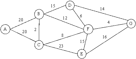
Question
Sarah and Jennifer have just graduated from college at the University of Washington in Seattle and want to go on a road trip.They have always wanted to see the mile-high city of Denver.Their road atlas shows the driving time (in hours)between various city pairs,as shown below.Formulate and solve a network optimization model to find the quickest route from Seattle to Denver? 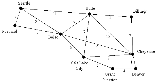
Question
Heart Beats is a manufacturer of medical equipment.The company's primary product is a device used to monitor the heart during medical procedures.This device is produced in two factories and shipped to two warehouses.The product is then shipped on demand to four third-party wholesalers.All shipping is done by truck.The product distribution network is shown below.The annual production capacity at Factories 1 and 2 is 400 and 250,respectively.The annual demand at Wholesalers 1,2,3,and 4 is 200,100,150,and 200,respectively.The cost of shipping one unit in each shipping lane is shown on the arcs.Due to limited truck capacity,at most 250 units can be shipped from Factory 1 to Warehouse 1 each year.Formulate and solve a network optimization model in a spreadsheet to determine how to distribute the product at the lowest possible annual cost. 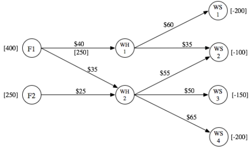

Unlock Deck
Sign up to unlock the cards in this deck!
Unlock Deck
Unlock Deck
1/3
Play
Full screen (f)
Deck 10: Network Optimization Models
Exxo 76 is an oil company that operates the pipeline network shown below,where each pipeline is labeled with its maximum flow rate in million cubic feet (MMcf)per day.A new oil well has been constructed near A.They would like to transport oil from the well near A to their refinery at G.Formulate and solve a network optimization model to determine the maximum flow rate from A to G.
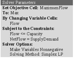
This is a maximum flow problem.Associated with each pipe in the network will be an arc (or,for pipes which might flow in either direction,two arcs,one in each direction).To set up a spreadsheet model,first list all of the arcs as shown in B5:C19,along with their capacity (F5:F19).Then list all of the nodes as shown in H5:H11.All the transshipment nodes (every node except the start node A and the end node G)will be constrained to have net flow = 0 (Supply/Demand = 0).The start node (A)and end node (G)are left unconstrained.We want to maximize the net flow out of node A. 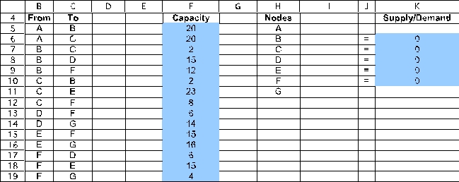 The changing cells are the amount of flow to send through each pipe (arc).These are shown in Flow (D5:D19)below,with an arbitrary value of 0 entered for each.The flow through each arc is capacitated as indicated by the <= in E5:E19.
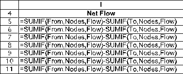
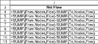
 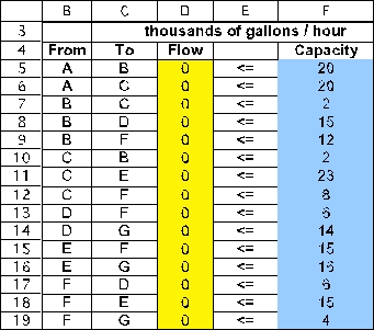 For each node,calculate the net flow as a function of the changing cells.This can be done using the SUMIF function.In each case,the first SUMIF function calculates the flow leaving the node and the second one calculates the flow entering the node.For example,consider the A node (H5).SUMIF(From,Nodes,Flow)in I5 sums each individual entry in Flow (the changing cells in D5:D19)if that entry is in a row where the entry in From (B5:B19)is the same as in the entry in that row of Nodes are rows 5 and 6,the sum in the ship column is only over these same rows,so this sum is D5+D6.
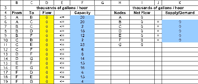
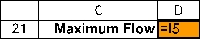
 The goal is to maximize the amount shipped from A to G.Since nodes B through F are transshipment nodes (net flow = 0),any amount that leaves A must enter G.Thus,maximizing the flow out of A will achieve our goal.Thus,the formula entered into the objective cell MaximumFlow (D21)is =I5.
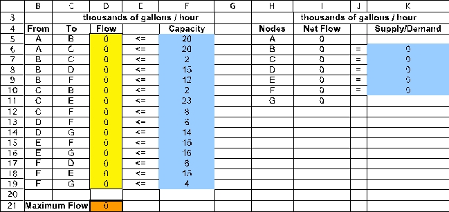
 The Solver information and solved spreadsheet are shown below.
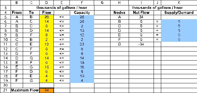

 Thus,Flow (D5:D19)indicates how to send oil through the network so as to achieve the Maximum Flow (D21)of 34 thousand gallons/hour.
The changing cells are the amount of flow to send through each pipe (arc).These are shown in Flow (D5:D19)below,with an arbitrary value of 0 entered for each.The flow through each arc is capacitated as indicated by the <= in E5:E19. For each node,calculate the net flow as a function of the changing cells.This can be done using the SUMIF function.In each case,the first SUMIF function calculates the flow leaving the node and the second one calculates the flow entering the node.For example,consider the A node (H5).SUMIF(From,Nodes,Flow)in I5 sums each individual entry in Flow (the changing cells in D5:D19)if that entry is in a row where the entry in From (B5:B19)is the same as in the entry in that row of Nodes are rows 5 and 6,the sum in the ship column is only over these same rows,so this sum is D5+D6. The goal is to maximize the amount shipped from A to G.Since nodes B through F are transshipment nodes (net flow = 0),any amount that leaves A must enter G.Thus,maximizing the flow out of A will achieve our goal.Thus,the formula entered into the objective cell MaximumFlow (D21)is =I5. The Solver information and solved spreadsheet are shown below. Thus,Flow (D5:D19)indicates how to send oil through the network so as to achieve the Maximum Flow (D21)of 34 thousand gallons/hour.Sarah and Jennifer have just graduated from college at the University of Washington in Seattle and want to go on a road trip.They have always wanted to see the mile-high city of Denver.Their road atlas shows the driving time (in hours)between various city pairs,as shown below.Formulate and solve a network optimization model to find the quickest route from Seattle to Denver?
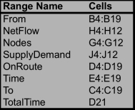
This is a shortest path problem.To set up a spreadsheet model,first list all of the arcs as shown in B4:C19,along with their travel time (E4:E19).Then list all of the nodes as shown in G4:G12 along with each node's supply or demand (J4:J12).We are sending one unit (Sarah and Jennifer's car)from Seattle to Denver,so the supply is 1 at Seattle and the demand is 1 at Denver.Every other node has demand 0 because if you enter the node,you must also leave it. 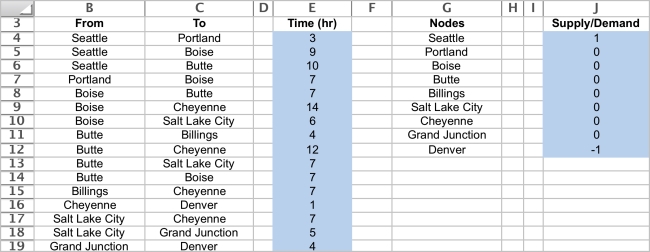 The changing cells are whether or not to include an arc on the route.These are shown in OnRoute (D4:D19)below.If the one unit (Sarah and Jennifer's car)is shipped through an arc,it must mean they traveled along that route.
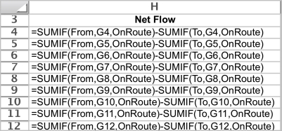
 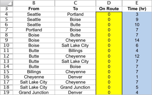 For each node,calculate the net flow as a function of the changing cells.This can be done using the SUMIF function.In each case,the first SUMIF function calculates the flow leaving the node and the second one calculates the flow entering the node.For example,consider the Seattle node (H4).SUMIF(From,G4,OnRoute)sums each individual entry in OnRoute (the changing cells in D4:D19)if that entry is in a row where the entry in From (B4:B19)is the same as in G4 are rows 4,5,and 6,the sum in the OnRoute column is only over these same rows,so this sum is D4+D5+D6.
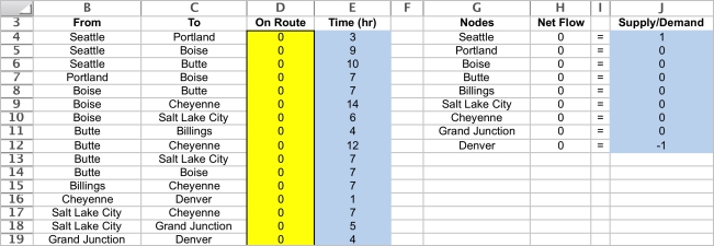
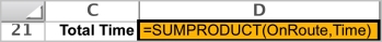
 The goal is to minimize the total time of the route.The cost is the SUMPRODUCT of the Time with OnRoute,or Total Time = SUMPRODUCT(OnRoute,Time).This formula is entered into TotalTime (D21).
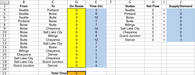
 The Solver information and solved spreadsheet are shown below.
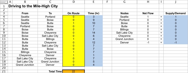
 OnRoute (D4:D19)indicates whether that arc should be included in the route.The optimal route is to go Seattle-Butte-Billings-Cheyenne-Denver.The minimum TotalTime (D21)is 22 hours.
The changing cells are whether or not to include an arc on the route.These are shown in OnRoute (D4:D19)below.If the one unit (Sarah and Jennifer's car)is shipped through an arc,it must mean they traveled along that route. For each node,calculate the net flow as a function of the changing cells.This can be done using the SUMIF function.In each case,the first SUMIF function calculates the flow leaving the node and the second one calculates the flow entering the node.For example,consider the Seattle node (H4).SUMIF(From,G4,OnRoute)sums each individual entry in OnRoute (the changing cells in D4:D19)if that entry is in a row where the entry in From (B4:B19)is the same as in G4 are rows 4,5,and 6,the sum in the OnRoute column is only over these same rows,so this sum is D4+D5+D6. The goal is to minimize the total time of the route.The cost is the SUMPRODUCT of the Time with OnRoute,or Total Time = SUMPRODUCT(OnRoute,Time).This formula is entered into TotalTime (D21). The Solver information and solved spreadsheet are shown below. OnRoute (D4:D19)indicates whether that arc should be included in the route.The optimal route is to go Seattle-Butte-Billings-Cheyenne-Denver.The minimum TotalTime (D21)is 22 hours.Heart Beats is a manufacturer of medical equipment.The company's primary product is a device used to monitor the heart during medical procedures.This device is produced in two factories and shipped to two warehouses.The product is then shipped on demand to four third-party wholesalers.All shipping is done by truck.The product distribution network is shown below.The annual production capacity at Factories 1 and 2 is 400 and 250,respectively.The annual demand at Wholesalers 1,2,3,and 4 is 200,100,150,and 200,respectively.The cost of shipping one unit in each shipping lane is shown on the arcs.Due to limited truck capacity,at most 250 units can be shipped from Factory 1 to Warehouse 1 each year.Formulate and solve a network optimization model in a spreadsheet to determine how to distribute the product at the lowest possible annual cost.
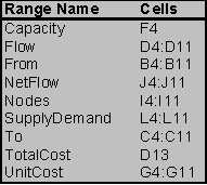
This is a minimum-cost flow problem.To set up a spreadsheet model,first list all of the arcs as shown in B4:C11,along with their capacity (F4)and unit cost (G4:G11).Only the arc from F1 to WH1 is capacitated.Then list all of the nodes as shown in I4:I11 along with each node's supply or demand (L4:L11). 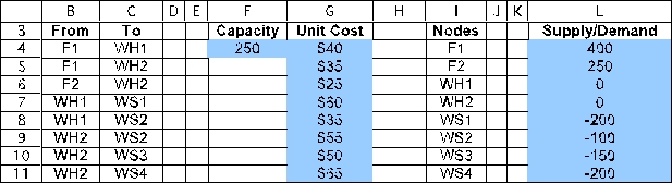 The changing cells are the amount of flow to send through each arc.These are shown in Flow (D4:D11)below,with an arbitrary value of 10 entered for each.The flow through the arc from F1 to WH1 must be less than the capacity of 250,as indicated by the constraint D4 <= F4.
 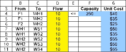 For each node,calculate the net flow as a function of the changing cells.This can be done using the SUMIF function.In each case,the first SUMIF function calculates the flow leaving the node and the second one calculates the flow entering the node.For example,consider the F1 node (I4).SUMIF(From,Nodes,Flow)sums each individual entry in Flow (the changing cells in D4:D11)if that entry is in a row where the entry in From (B4:B11)is the same as in that row of Nodes are rows 4 and 5,the sum in the ship column is only over these same rows,so this sum is D4+D5.
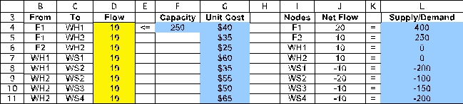
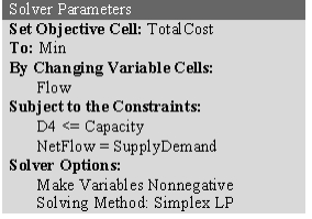
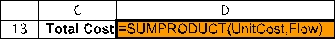
 The goal is to minimize the total cost of shipping the product from the factories to the wholesalers.The cost is the SUMPRODUCT of the Unit Costs with the Flow,or Total Cost = SUMPRODUCT(UnitCost,Flow).This formula is entered into TotalCost (D13).
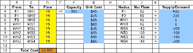
 The Solver information and solved spreadsheet are shown below.
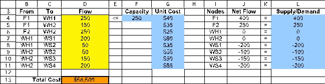

 Thus,Flow (D4:D11)indicates how to distribute the product so as to achieve the minimum Total Cost (D13)of $58,500.
The changing cells are the amount of flow to send through each arc.These are shown in Flow (D4:D11)below,with an arbitrary value of 10 entered for each.The flow through the arc from F1 to WH1 must be less than the capacity of 250,as indicated by the constraint D4 <= F4. For each node,calculate the net flow as a function of the changing cells.This can be done using the SUMIF function.In each case,the first SUMIF function calculates the flow leaving the node and the second one calculates the flow entering the node.For example,consider the F1 node (I4).SUMIF(From,Nodes,Flow)sums each individual entry in Flow (the changing cells in D4:D11)if that entry is in a row where the entry in From (B4:B11)is the same as in that row of Nodes are rows 4 and 5,the sum in the ship column is only over these same rows,so this sum is D4+D5. The goal is to minimize the total cost of shipping the product from the factories to the wholesalers.The cost is the SUMPRODUCT of the Unit Costs with the Flow,or Total Cost = SUMPRODUCT(UnitCost,Flow).This formula is entered into TotalCost (D13). The Solver information and solved spreadsheet are shown below. Thus,Flow (D4:D11)indicates how to distribute the product so as to achieve the minimum Total Cost (D13)of $58,500. Unlock Deck
Unlock for access to all 3 flashcards in this deck.


