Deck 3: Review of Statistics
Full screen (f)
Question
Question
A large p-value implies
A)rejection of the null hypothesis.
B)a large t-statistic.
C)a large act.
act.
D)that the observed value act is consistent with the null hypothesis.
A)rejection of the null hypothesis.
B)a large t-statistic.
C)a large
act.D)that the observed value
act is consistent with the null hypothesis. Question
The standard error of  is given by the following formula:
A) .
.
B) .
.
C) .
.
D) .
.
is given by the following formula:A)
.B)
.C)
.D)
. Question
Question
Question
Question
To derive the least squares estimator µY,you find the estimator m which minimizes
A) .
.
B) .
.
C) .
.
D) .
.
A)
.B)
.C)
.D)
. Question
The p-value is defined as follows:
A)p = 0.05.
B)PrH0 [![<strong>The p-value is defined as follows:</strong> A)p = 0.05. B)PrH0 [ - µY,0 > act - µY,0 ]. C)Pr(z > 1.96). D)PrH0 [ - µY,0 < act - µY,0 ]. <div style=padding-top: 35px>](https://d2lvgg3v3hfg70.cloudfront.net/TB2833/11eab146_bd38_bad0_896a_67dc45cc679f_TB2833_11.jpg)
![<strong>The p-value is defined as follows:</strong> A)p = 0.05. B)PrH0 [ - µY,0 > act - µY,0 ]. C)Pr(z > 1.96). D)PrH0 [ - µY,0 < act - µY,0 ]. <div style=padding-top: 35px>](https://d2lvgg3v3hfg70.cloudfront.net/TB2833/11eab146_bd38_bad1_896a_1fea5aec05f2_TB2833_11.jpg) - µY,0
- µY,0
![<strong>The p-value is defined as follows:</strong> A)p = 0.05. B)PrH0 [ - µY,0 > act - µY,0 ]. C)Pr(z > 1.96). D)PrH0 [ - µY,0 < act - µY,0 ]. <div style=padding-top: 35px>](https://d2lvgg3v3hfg70.cloudfront.net/TB2833/11eab146_bd38_bad2_896a_79d789cded2e_TB2833_11.jpg) >
>
![<strong>The p-value is defined as follows:</strong> A)p = 0.05. B)PrH0 [ - µY,0 > act - µY,0 ]. C)Pr(z > 1.96). D)PrH0 [ - µY,0 < act - µY,0 ]. <div style=padding-top: 35px>](https://d2lvgg3v3hfg70.cloudfront.net/TB2833/11eab146_bd38_bad3_896a_ebfb3fb3d9f6_TB2833_11.jpg)
![<strong>The p-value is defined as follows:</strong> A)p = 0.05. B)PrH0 [ - µY,0 > act - µY,0 ]. C)Pr(z > 1.96). D)PrH0 [ - µY,0 < act - µY,0 ]. <div style=padding-top: 35px>](https://d2lvgg3v3hfg70.cloudfront.net/TB2833/11eab146_bd38_bad4_896a_a73958c03aa8_TB2833_11.jpg) act - µY,0
act - µY,0
![<strong>The p-value is defined as follows:</strong> A)p = 0.05. B)PrH0 [ - µY,0 > act - µY,0 ]. C)Pr(z > 1.96). D)PrH0 [ - µY,0 < act - µY,0 ]. <div style=padding-top: 35px>](https://d2lvgg3v3hfg70.cloudfront.net/TB2833/11eab146_bd38_e1e5_896a_919a811c2477_TB2833_11.jpg) ].
].
C)Pr(z > 1.96).
D)PrH0 [![<strong>The p-value is defined as follows:</strong> A)p = 0.05. B)PrH0 [ - µY,0 > act - µY,0 ]. C)Pr(z > 1.96). D)PrH0 [ - µY,0 < act - µY,0 ]. <div style=padding-top: 35px>](https://d2lvgg3v3hfg70.cloudfront.net/TB2833/11eab146_bd38_e1e6_896a_2bb017106bbc_TB2833_11.jpg)
![<strong>The p-value is defined as follows:</strong> A)p = 0.05. B)PrH0 [ - µY,0 > act - µY,0 ]. C)Pr(z > 1.96). D)PrH0 [ - µY,0 < act - µY,0 ]. <div style=padding-top: 35px>](https://d2lvgg3v3hfg70.cloudfront.net/TB2833/11eab146_bd38_e1e7_896a_4f643bd78015_TB2833_11.jpg) - µY,0
- µY,0
![<strong>The p-value is defined as follows:</strong> A)p = 0.05. B)PrH0 [ - µY,0 > act - µY,0 ]. C)Pr(z > 1.96). D)PrH0 [ - µY,0 < act - µY,0 ]. <div style=padding-top: 35px>](https://d2lvgg3v3hfg70.cloudfront.net/TB2833/11eab146_bd38_e1e8_896a_211c346f80f3_TB2833_11.jpg) <
<
![<strong>The p-value is defined as follows:</strong> A)p = 0.05. B)PrH0 [ - µY,0 > act - µY,0 ]. C)Pr(z > 1.96). D)PrH0 [ - µY,0 < act - µY,0 ]. <div style=padding-top: 35px>](https://d2lvgg3v3hfg70.cloudfront.net/TB2833/11eab146_bd38_e1e9_896a_05609fc8200e_TB2833_11.jpg)
![<strong>The p-value is defined as follows:</strong> A)p = 0.05. B)PrH0 [ - µY,0 > act - µY,0 ]. C)Pr(z > 1.96). D)PrH0 [ - µY,0 < act - µY,0 ]. <div style=padding-top: 35px>](https://d2lvgg3v3hfg70.cloudfront.net/TB2833/11eab146_bd38_e1ea_896a_c1895441d6ad_TB2833_11.jpg) act - µY,0
act - µY,0
![<strong>The p-value is defined as follows:</strong> A)p = 0.05. B)PrH0 [ - µY,0 > act - µY,0 ]. C)Pr(z > 1.96). D)PrH0 [ - µY,0 < act - µY,0 ]. <div style=padding-top: 35px>](https://d2lvgg3v3hfg70.cloudfront.net/TB2833/11eab146_bd39_08fb_896a_c3423a6a10b6_TB2833_11.jpg) ].
].
A)p = 0.05.
B)PrH0 [
- µY,0 > act - µY,0 ].C)Pr(z > 1.96).
D)PrH0 [
- µY,0 < act - µY,0 ]. Question
When you are testing a hypothesis against a two-sided alternative,then the alternative is written as
A)E(Y)> µY,0.
B)E(Y)= µY,0.
C) ≠ µY,0.
D)E(Y)≠ µY,0.
A)E(Y)> µY,0.
B)E(Y)= µY,0.
C)
≠ µY,0.D)E(Y)≠ µY,0.
Question
An estimator  of the population value
  is more efficient when compared to another estimator
  ,if
,if
A)E( )> E(
)> E(
 ).
).
B)it has a smaller variance.
C)its c.d.f.is flatter than that of the other estimator.
D)both estimators are unbiased,and var( )< var(
 ).
).
of the population value is more efficient when compared to another estimator ,ifA)E(
)> E( ).B)it has a smaller variance.
C)its c.d.f.is flatter than that of the other estimator.
D)both estimators are unbiased,and var(
)< var( ). Question
Question
Question
An estimator  of the population value
  is unbiased if
A) =
=
 .
.
B) has the smallest variance of all estimators.
C) .
.
D)E( )=
)=
 .
.
of the population value is unbiased ifA)
= .B)
has the smallest variance of all estimators.C)
.D)E(
)= . Question
Among all unbiased estimators that are weighted averages of Y1,... ,Yn  ,is
,is
A)the only consistent estimator of µY.
B)the most efficient estimator of µY.
C)a number which,by definition,cannot have a variance.
D)the most unbiased estimator of µY.
,isA)the only consistent estimator of µY.
B)the most efficient estimator of µY.
C)a number which,by definition,cannot have a variance.
D)the most unbiased estimator of µY.
Question
Question
If the null hypothesis states H0 : E(Y)= µY,0,then a two-sided alternative hypothesis is
A)H1 : E(Y)≠ µY,0.
B)H1 : E(Y)≈ µY,0.
C)H1 : < µY,0.
D)H1 : E(Y)> µY,0.
A)H1 : E(Y)≠ µY,0.
B)H1 : E(Y)≈ µY,0.
C)H1 :
< µY,0.D)H1 : E(Y)> µY,0.
Question
Question
An estimator  of the population value
  is consistent if
A)

 .
.
B)its mean square error is the smallest possible.
C)Y is normally distributed.
D) .
.
of the population value is consistent ifA)
.B)its mean square error is the smallest possible.
C)Y is normally distributed.
D)
. Question
Question
With i.i.d.sampling each of the following is true except
A)E =
=
 .
.
B)var =
=
 /n.
/n.
C)E < E(Y).
D) is a random variable.
A)E
= .B)var
= /n.C)E
< E(Y).D)
is a random variable. Question
Degrees of freedom
A)in the context of the sample variance formula means that estimating the mean uses up some of the information in the data.
B)is something that certain undergraduate majors at your university/college other than economics seem to have an ∞ amount of.
C)are (n-2)when replacing the population mean by the sample mean.
D)ensure that .
.
A)in the context of the sample variance formula means that estimating the mean uses up some of the information in the data.
B)is something that certain undergraduate majors at your university/college other than economics seem to have an ∞ amount of.
C)are (n-2)when replacing the population mean by the sample mean.
D)ensure that
. Question
When testing for differences of means,the t-statistic t =  , where
 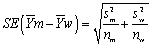 has
has
A)a student t distribution if the population distribution of Y is not normal
B)a student t distribution if the population distribution of Y is normal
C)a normal distribution even in small samples
D)cannot be computed unless =
=

, where hasA)a student t distribution if the population distribution of Y is not normal
B)a student t distribution if the population distribution of Y is normal
C)a normal distribution even in small samples
D)cannot be computed unless
= Question
The standard error for the difference in means if two random variables M and W,when the two population variances are different,is
A) .
.
B) .
.
C) .
.
D) .
.
A)
.B)
.C)
.D)
. Question
When testing for differences of means,you can base statistical inference on the
A)Student t distribution in general
B)normal distribution regardless of sample size
C)Student t distribution if the underlying population distribution of Y is normal,the two groups have the same variances,and you use the pooled standard error formula
D)Chi-squared distribution with ( +
+
 - 2)degrees of freedom
A)Student t distribution in general
B)normal distribution regardless of sample size
C)Student t distribution if the underlying population distribution of Y is normal,the two groups have the same variances,and you use the pooled standard error formula
D)Chi-squared distribution with (
+ - 2)degrees of freedom Question
Assume that two presidential candidates,call them Bush and Gore,receive 50% of the votes in the population.You can model this situation as a Bernoulli trial,where Y is a random variable with success probability Pr(Y = 1)= p,and where Y = 1 if a person votes for Bush and Y = 0 otherwise.Furthermore,let  be the fraction of successes (1s)in a sample,which is distributed N(p,
  )in reasonably large samples,say for n ≥ 40.
(a)Given your knowledge about the population,find the probability that in a random sample of 40,Bush would receive a share of 40% or less.
(b)How would this situation change with a random sample of 100?
(c)Given your answers in (a)and (b),would you be comfortable to predict what the voting intentions for the entire population are if you did not know p but had polled 10,000 individuals at random and calculated ? Explain.
(d)This result seems to hold whether you poll 10,000 people at random in the Netherlands or the United States,where the former has a population of less than 20 million people,while the United States is 15 times as populous.Why does the population size not come into play?
be the fraction of successes (1s)in a sample,which is distributed N(p, )in reasonably large samples,say for n ≥ 40.(a)Given your knowledge about the population,find the probability that in a random sample of 40,Bush would receive a share of 40% or less.
(b)How would this situation change with a random sample of 100?
(c)Given your answers in (a)and (b),would you be comfortable to predict what the voting intentions for the entire population are if you did not know p but had polled 10,000 individuals at random and calculated
? Explain.(d)This result seems to hold whether you poll 10,000 people at random in the Netherlands or the United States,where the former has a population of less than 20 million people,while the United States is 15 times as populous.Why does the population size not come into play?
Question
Assume that you have 125 observations on the height (H)and weight (W)of your peers in college. Let  = 68,
= 68,  = 3.5,
  = 29.The sample correlation coefficient is
A)1.22
B)0.50
C)0.67
D)Cannot be computed since males and females have not been separated out.
= 68, = 3.5, = 29.The sample correlation coefficient isA)1.22
B)0.50
C)0.67
D)Cannot be computed since males and females have not been separated out.
Question
When the sample size n is large,the 90% confidence interval for  is
is
A) ± 1.96SE(
 ).
).
B) ± 1.64SE(
 ).
).
C) ± 1.64
 .
.
D) ± 1.96.
isA)
± 1.96SE( ).B)
± 1.64SE( ).C)
± 1.64 .D)
± 1.96. Question
You have collected data on the average weekly amount of studying time (T)and grades (G)from the peers at your college.Changing the measurement from minutes into hours has the following effect on the correlation coefficient:
A)decreases the by dividing the original correlation coefficient by 60
B)results in a higher
C)cannot be computed since some students study less than an hour per week
D)does not change the
A)decreases the
by dividing the original correlation coefficient by 60B)results in a higher
C)cannot be computed since some students study less than an hour per week
D)does not change the
Question
Math SAT scores (Y)are normally distributed with a mean of 500 and a standard deviation of 100.An evening school advertises that it can improve students' scores by roughly a third of a standard deviation,or 30 points,if they attend a course which runs over several weeks.(A similar claim is made for attending a verbal SAT course. )The statistician for a consumer protection agency suspects that the courses are not effective.She views the situation as follows: H0 :  = 500 vs.H1 :
  = 530.
(a)Sketch the two distributions under the null hypothesis and the alternative hypothesis.
(b)The consumer protection agency wants to evaluate this claim by sending 50 students to attend classes.One of the students becomes sick during the course and drops out.What is the distribution of the average score of the remaining 49 students under the null,and under the alternative hypothesis?
(c)Assume that after graduating from the course,the 49 participants take the SAT test and score an average of 520.Is this convincing evidence that the school has fallen short of its claim? What is the p-value for such a score under the null hypothesis?
(d)What would be the critical value under the null hypothesis if the size of your test were 5%?
(e)Given this critical value,what is the power of the test? What options does the statistician have for increasing the power in this situation?
= 500 vs.H1 : = 530.(a)Sketch the two distributions under the null hypothesis and the alternative hypothesis.
(b)The consumer protection agency wants to evaluate this claim by sending 50 students to attend classes.One of the students becomes sick during the course and drops out.What is the distribution of the average score of the remaining 49 students under the null,and under the alternative hypothesis?
(c)Assume that after graduating from the course,the 49 participants take the SAT test and score an average of 520.Is this convincing evidence that the school has fallen short of its claim? What is the p-value for such a score under the null hypothesis?
(d)What would be the critical value under the null hypothesis if the size of your test were 5%?
(e)Given this critical value,what is the power of the test? What options does the statistician have for increasing the power in this situation?
Question
The sample covariance can be calculated in any of the following ways,with the exception of:
A)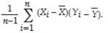
B)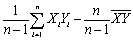 .
.
C)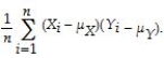
D)rXYSYSY,where rXY is the correlation coefficient.
A)
B)
.C)
D)rXYSYSY,where rXY is the correlation coefficient.
Question
Question
Question
Adult males are taller,on average,than adult females.Visiting two recent American Youth Soccer Organization (AYSO)under 12 year old (U12)soccer matches on a Saturday,you do not observe an obvious difference in the height of boys and girls of that age.You suggest to your little sister that she collect data on height and gender of children in 4th to 6th grade as part of her science project.The accompanying table shows her findings.
Height of Young Boys and Girls,Grades 4-6,in inches
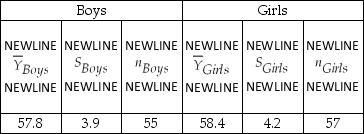 (a)Let your null hypothesis be that there is no difference in the height of females and males at this age level.Specify the alternative hypothesis.
(b)Find the difference in height and the standard error of the difference.
(c)Generate a 95% confidence interval for the difference in height.
(d)Calculate the t-statistic for comparing the two means.Is the difference statistically significant at the 1% level? Which critical value did you use? Why would this number be smaller if you had assumed a one-sided alternative hypothesis? What is the intuition behind this?
Height of Young Boys and Girls,Grades 4-6,in inches
(a)Let your null hypothesis be that there is no difference in the height of females and males at this age level.Specify the alternative hypothesis.(b)Find the difference in height and the standard error of the difference.
(c)Generate a 95% confidence interval for the difference in height.
(d)Calculate the t-statistic for comparing the two means.Is the difference statistically significant at the 1% level? Which critical value did you use? Why would this number be smaller if you had assumed a one-sided alternative hypothesis? What is the intuition behind this?
Question
The formula for the sample variance is
A)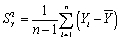 .
.
B)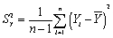 .
.
C)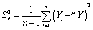 .
.
D)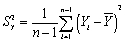 .
.
A)
.B)
.C)
.D)
. Question
Question
Your packaging company fills various types of flour into bags.Recently there have been complaints from one chain of stores: a customer returned one opened 5 pound bag which weighed significantly less than the label indicated.You view the weight of the bag as a random variable which is normally distributed with a mean of 5 pounds,and,after studying the machine specifications,a standard deviation of 0.05 pounds.
(a)You take a sample of 20 bags and weigh them.Sketch below what the average pattern of individual weights might look like.Let the horizontal axis indicate the sampled bag number (1,2,…,20).On the vertical axis,mark the expected value of the weight under the null hypothesis,and two (≈ 1.96)standard deviations above and below the expected value.Draw a line through the graph for E(Y)+ 2 ,E(Y),and E(Y)- 2
  .How many of the bags in a sample of 20 will you expect to weigh either less than 4.9 pounds or more than 5.1 pounds?
(b)You sample 25 bags of flour and calculate the average weight.What is the distribution of the average weight of these 25 bags? Repeating the same exercise 20 times,sketch what the distribution of the average weights would look like in a graph similar to the one you drew in (b),where you have adjusted the standard error of accordingly.
(c)For each of the twenty observations in (c)a 95% confidence interval is constructed.Draw these confidence intervals,using the same graph as in (c).How many of these 20 confidence intervals would you expect to weigh 5 pounds under the null hypothesis?
(a)You take a sample of 20 bags and weigh them.Sketch below what the average pattern of individual weights might look like.Let the horizontal axis indicate the sampled bag number (1,2,…,20).On the vertical axis,mark the expected value of the weight under the null hypothesis,and two (≈ 1.96)standard deviations above and below the expected value.Draw a line through the graph for E(Y)+ 2
,E(Y),and E(Y)- 2 .How many of the bags in a sample of 20 will you expect to weigh either less than 4.9 pounds or more than 5.1 pounds?(b)You sample 25 bags of flour and calculate the average weight.What is the distribution of the average weight of these 25 bags? Repeating the same exercise 20 times,sketch what the distribution of the average weights would look like in a graph similar to the one you drew in (b),where you have adjusted the standard error of
accordingly.(c)For each of the twenty observations in (c)a 95% confidence interval is constructed.Draw these confidence intervals,using the same graph as in (c).How many of these 20 confidence intervals would you expect to weigh 5 pounds under the null hypothesis?
Question
The power of the test
A)is the probability that the test actually incorrectly rejects the null hypothesis when the null is true.
B)depends on whether you use or
or
 2 for the t-statistic.
C)is one minus the size of the test.
D)is the probability that the test correctly rejects the null when the alternative is true.
A)is the probability that the test actually incorrectly rejects the null hypothesis when the null is true.
B)depends on whether you use
or 2 for the t-statistic.C)is one minus the size of the test.
D)is the probability that the test correctly rejects the null when the alternative is true.
Question
Question
The t-statistic is defined as follows:
A) .
.
B) .
.
C) .
.
D)1.96.
A)
.B)
.C)
.D)1.96.
Question
The following statement about the sample correlation coefficient is true.
A)-1 ≤ rX,Y ≤ 1.
B)
 corr(Xi,Yi).
C)| rX,Y | < 1.
D)rX,Y = .
.
A)-1 ≤ rX,Y ≤ 1.
B)
corr(Xi,Yi).C)| rX,Y | < 1.
D)rX,Y =
. Question
Your textbook states that when you test for differences in means and you assume that the two population variances are equal,then an estimator of the population variance is the following "pooled" estimator: 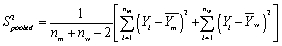 Explain why this pooled estimator can be looked at as the weighted average of the two variances.
Explain why this pooled estimator can be looked at as the weighted average of the two variances. Question
During the last few days before a presidential election,there is a frenzy of voting intention surveys.On a given day,quite often there are conflicting results from three major polls.
(a)Think of each of these polls as reporting the fraction of successes (1s)of a Bernoulli random variable Y,where the probability of success is Pr(Y = 1)= p.Let be the fraction of successes in the sample and assume that this estimator is normally distributed with a mean of p and a variance of
  .Why are the results for all polls different,even though they are taken on the same day?
(b)Given the estimator of the variance of ,
,  ,construct a 95% confidence interval for
  .For which value of
  is the standard deviation the largest? What value does it take in the case of a maximum
  ?
?
(c)When the results from the polls are reported,you are told,typically in the small print,that the "margin of error" is plus or minus two percentage points.Using the approximation of 1.96 ≈ 2,and assuming,"conservatively," the maximum standard deviation derived in (b),what sample size is required to add and subtract ("margin of error")two percentage points from the point estimate?
(d)What sample size would you need to halve the margin of error?
(a)Think of each of these polls as reporting the fraction of successes (1s)of a Bernoulli random variable Y,where the probability of success is Pr(Y = 1)= p.Let
be the fraction of successes in the sample and assume that this estimator is normally distributed with a mean of p and a variance of .Why are the results for all polls different,even though they are taken on the same day?(b)Given the estimator of the variance of
, ,construct a 95% confidence interval for .For which value of is the standard deviation the largest? What value does it take in the case of a maximum ?(c)When the results from the polls are reported,you are told,typically in the small print,that the "margin of error" is plus or minus two percentage points.Using the approximation of 1.96 ≈ 2,and assuming,"conservatively," the maximum standard deviation derived in (b),what sample size is required to add and subtract ("margin of error")two percentage points from the point estimate?
(d)What sample size would you need to halve the margin of error?
Question
Question
Let Y be a Bernoulli random variable with success probability Pr(Y = 1)= p,and let Y1,... ,Yn be i.i.d.draws from this distribution.Let  be the fraction of successes (1s)in this sample.In large samples,the distribution of
  will be approximately normal,i.e. ,
  is approximately distributed N(p,
  ).Now let X be the number of successes and n the sample size.In a sample of 10 voters (n=10),if there are six who vote for candidate A,then X = 6.Relate X,the number of success,to
  ,the success proportion,or fraction of successes.Next,using your knowledge of linear transformations,derive the distribution of X.
be the fraction of successes (1s)in this sample.In large samples,the distribution of will be approximately normal,i.e. , is approximately distributed N(p, ).Now let X be the number of successes and n the sample size.In a sample of 10 voters (n=10),if there are six who vote for candidate A,then X = 6.Relate X,the number of success,to ,the success proportion,or fraction of successes.Next,using your knowledge of linear transformations,derive the distribution of X. Question
Question
Let p be the success probability of a Bernoulli random variable Y,i.e. ,p = Pr(Y = 1).It can be shown that  ,the fraction of successes in a sample,is asymptotically distributed N(p,
  .Using the estimator of the variance of
  ,
,  ,construct a 95% confidence interval for p.Show that the margin for sampling error simplifies to 1/
  if you used 2 instead of 1.96 assuming,conservatively,that the standard error is at its maximum.Construct a table indicating the sample size needed to generate a margin of sampling error of 1%,2%,5% and 10%.What do you notice about the increase in sample size needed to halve the margin of error? (The margin of sampling error is 1.96×SE(
  ))
))
,the fraction of successes in a sample,is asymptotically distributed N(p, .Using the estimator of the variance of , ,construct a 95% confidence interval for p.Show that the margin for sampling error simplifies to 1/ if you used 2 instead of 1.96 assuming,conservatively,that the standard error is at its maximum.Construct a table indicating the sample size needed to generate a margin of sampling error of 1%,2%,5% and 10%.What do you notice about the increase in sample size needed to halve the margin of error? (The margin of sampling error is 1.96×SE( )) Question
Question
The development office and the registrar have provided you with anonymous matches of starting salaries and GPAs for 108 graduating economics majors.Your sample contains a variety of jobs,from church pastor to stockbroker.
(a)The average starting salary for the 108 students was $38,644.86 with a standard deviation of $7,541.40.Construct a 95% confidence interval for the starting salary of all economics majors at your university/college.
(b)A similar sample for psychology majors indicates a significantly lower starting salary.Given that these students had the same number of years of education,does this indicate discrimination in the job market against psychology majors?
(c)You wonder if it pays (no pun intended)to get good grades by calculating the average salary for economics majors who graduated with a cumulative GPA of B+ or better,and those who had a B or worse.The data is as shown in the accompanying table.
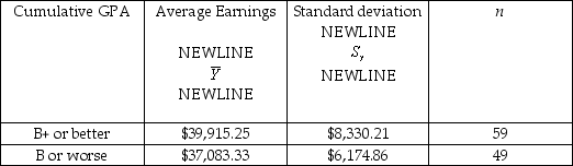 Conduct a t-test for the hypothesis that the two starting salaries are the same in the population.Given that this data was collected in 1999,do you think that your results will hold for other years,such as 2002?
(a)The average starting salary for the 108 students was $38,644.86 with a standard deviation of $7,541.40.Construct a 95% confidence interval for the starting salary of all economics majors at your university/college.
(b)A similar sample for psychology majors indicates a significantly lower starting salary.Given that these students had the same number of years of education,does this indicate discrimination in the job market against psychology majors?
(c)You wonder if it pays (no pun intended)to get good grades by calculating the average salary for economics majors who graduated with a cumulative GPA of B+ or better,and those who had a B or worse.The data is as shown in the accompanying table.
Conduct a t-test for the hypothesis that the two starting salaries are the same in the population.Given that this data was collected in 1999,do you think that your results will hold for other years,such as 2002? Question
Question
Some policy advisors have argued that education should be subsidized in developing countries to reduce fertility rates.To investigate whether or not education and fertility are correlated,you collect data on population growth rates (Y)and education (X)for 86 countries.Given the sums below,compute the sample correlation:  = 1.594;
  = 449.6;
  = 6.4697;
  = 0.03982;
  = 3,022.76
= 1.594; = 449.6; = 6.4697; = 0.03982; = 3,022.76 Question
Question
You have collected weekly earnings and age data from a sub-sample of 1,744 individuals using the Current Population Survey in a given year.
(a)Given the overall mean of $434.49 and a standard deviation of $294.67,construct a 99% confidence interval for average earnings in the entire population.State the meaning of this interval in words,rather than just in numbers.If you constructed a 90% confidence interval instead,would it be smaller or larger? What is the intuition?
(b)When dividing your sample into people 45 years and older,and younger than 45,the information shown in the table is found.
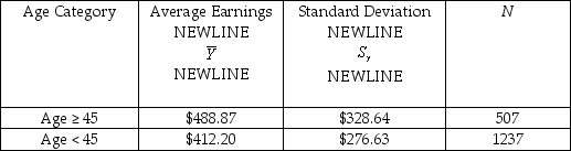 Test whether or not the difference in average earnings is statistically significant.Given your knowledge of age-earning profiles,does this result make sense?
(a)Given the overall mean of $434.49 and a standard deviation of $294.67,construct a 99% confidence interval for average earnings in the entire population.State the meaning of this interval in words,rather than just in numbers.If you constructed a 90% confidence interval instead,would it be smaller or larger? What is the intuition?
(b)When dividing your sample into people 45 years and older,and younger than 45,the information shown in the table is found.
Test whether or not the difference in average earnings is statistically significant.Given your knowledge of age-earning profiles,does this result make sense? Question
U.S.News and World Report ranks colleges and universities annually.You randomly sample 100 of the national universities and liberal arts colleges from the year 2000 issue.The average cost,which includes tuition,fees,and room and board,is $23,571.49 with a standard deviation of $7,015.52.
(a)Based on this sample,construct a 95% confidence interval of the average cost of attending a university/college in the United States.
(b)Cost varies by quite a bit.One of the reasons may be that some universities/colleges have a better reputation than others.U.S.News and World Reports tries to measure this factor by asking university presidents and chief academic officers about the reputation of institutions.The ranking is from 1 ("marginal")to 5 ("distinguished").You decide to split the sample according to whether the academic institution has a reputation of greater than 3.5 or not.For comparison,in 2000,Caltech had a reputation ranking of 4.7,Smith College had 4.5,and Auburn University had 3.1.This gives you the statistics shown in the accompanying table.
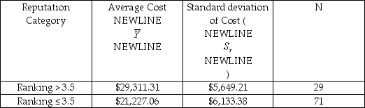 Test the hypothesis that the average cost for all universities/colleges is the same independent of the reputation.What alternative hypothesis did you use?
(c)What other factors should you consider before making a decision based on the data in (b)?
(a)Based on this sample,construct a 95% confidence interval of the average cost of attending a university/college in the United States.
(b)Cost varies by quite a bit.One of the reasons may be that some universities/colleges have a better reputation than others.U.S.News and World Reports tries to measure this factor by asking university presidents and chief academic officers about the reputation of institutions.The ranking is from 1 ("marginal")to 5 ("distinguished").You decide to split the sample according to whether the academic institution has a reputation of greater than 3.5 or not.For comparison,in 2000,Caltech had a reputation ranking of 4.7,Smith College had 4.5,and Auburn University had 3.1.This gives you the statistics shown in the accompanying table.
Test the hypothesis that the average cost for all universities/colleges is the same independent of the reputation.What alternative hypothesis did you use?(c)What other factors should you consider before making a decision based on the data in (b)?
Question
(Advanced)Unbiasedness and small variance are desirable properties of estimators.However,you can imagine situations where a trade-off exists between the two: one estimator may be have a small bias but a much smaller variance than another,unbiased estimator.The concept of "mean square error" estimator combines the two concepts.Let  be an estimator of μ.Then the mean square error (MSE)is defined as follows: MSE(
  )= E(
)= E(  - μ)2.Prove that MSE(
  )= bias2 + var(
  ).(Hint: subtract and add in E(
  )in E(
  - μ)2. )
be an estimator of μ.Then the mean square error (MSE)is defined as follows: MSE( )= E( - μ)2.Prove that MSE( )= bias2 + var( ).(Hint: subtract and add in E( )in E( - μ)2. ) Question
(Requires calculus. )Let Y be a Bernoulli random variable with success probability Pr(Y = 1)= p.It can be shown that the variance of the success probability p is  .Use calculus to show that this variance is maximized for p = 0.5.
.Use calculus to show that this variance is maximized for p = 0.5. Question
Question
When you perform hypothesis tests,you are faced with four possible outcomes described in the accompanying table. 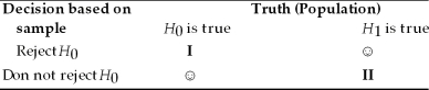 "☺" indicates a correct decision,and I and II indicate that an error has been made.In probability terms,state the mistakes that have been made in situation I and II,and relate these to the Size of the test and the Power of the test (or transformations of these).
"☺" indicates a correct decision,and I and II indicate that an error has been made.In probability terms,state the mistakes that have been made in situation I and II,and relate these to the Size of the test and the Power of the test (or transformations of these). Question
Question
Question
Assume that under the null hypothesis,  has an expected value of 500 and a standard deviation of 20.Under the alternative hypothesis,the expected value is 550.Sketch the probability density function for the null and the alternative hypothesis in the same figure.Pick a critical value such that the p-value is approximately 5%.Mark the areas,which show the size and the power of the test.What happens to the power of the test if the alternative hypothesis moves closer to the null hypothesis,i.e. ,,
  = 540,530,520,etc.?
has an expected value of 500 and a standard deviation of 20.Under the alternative hypothesis,the expected value is 550.Sketch the probability density function for the null and the alternative hypothesis in the same figure.Pick a critical value such that the p-value is approximately 5%.Mark the areas,which show the size and the power of the test.What happens to the power of the test if the alternative hypothesis moves closer to the null hypothesis,i.e. ,, = 540,530,520,etc.? Question
Question
Question

Unlock Deck
Sign up to unlock the cards in this deck!
Unlock Deck
Unlock Deck
1/63
Play
Full screen (f)
Deck 3: Review of Statistics
1
The size of the test
A)is the probability of committing a type I error.
B)is the same as the sample size.
C)is always equal to (1-the power of test).
D)can be greater than 1 in extreme examples.
A)is the probability of committing a type I error.
B)is the same as the sample size.
C)is always equal to (1-the power of test).
D)can be greater than 1 in extreme examples.
A
2
A large p-value implies
A)rejection of the null hypothesis.
B)a large t-statistic.
C)a large act.
D)that the observed value act is consistent with the null hypothesis.
A)rejection of the null hypothesis.
B)a large t-statistic.
C)a large
act.D)that the observed value
act is consistent with the null hypothesis.D
3
The standard error of is given by the following formula:
A) .
B) .
C) .
D) .
is given by the following formula:A)
.B)
.C)
.D)
.D
4
The critical value of a two-sided t-test computed from a large sample
A)is 1.64 if the significance level of the test is 5%.
B)cannot be calculated unless you know the degrees of freedom.
C)is 1.96 if the significance level of the test is 5%.
D)is the same as the p-value.
A)is 1.64 if the significance level of the test is 5%.
B)cannot be calculated unless you know the degrees of freedom.
C)is 1.96 if the significance level of the test is 5%.
D)is the same as the p-value.
Unlock Deck
Unlock for access to all 63 flashcards in this deck.
Unlock Deck
k this deck
5
A type II error
A)is typically smaller than the type I error.
B)is the error you make when choosing type II or type I.
C)is the error you make when not rejecting the null hypothesis when it is false.
D)cannot be calculated when the alternative hypothesis contains an "=".
A)is typically smaller than the type I error.
B)is the error you make when choosing type II or type I.
C)is the error you make when not rejecting the null hypothesis when it is false.
D)cannot be calculated when the alternative hypothesis contains an "=".
Unlock Deck
Unlock for access to all 63 flashcards in this deck.
Unlock Deck
k this deck
6
The power of the test is
A)dependent on whether you calculate a t or a t2 statistic.
B)one minus the probability of committing a type I error.
C)a subjective view taken by the econometrician dependent on the situation.
D)one minus the probability of committing a type II error.
A)dependent on whether you calculate a t or a t2 statistic.
B)one minus the probability of committing a type I error.
C)a subjective view taken by the econometrician dependent on the situation.
D)one minus the probability of committing a type II error.
Unlock Deck
Unlock for access to all 63 flashcards in this deck.
Unlock Deck
k this deck
7
To derive the least squares estimator µY,you find the estimator m which minimizes
A) .
B) .
C) .
D) .
A)
.B)
.C)
.D)
. Unlock Deck
Unlock for access to all 63 flashcards in this deck.
Unlock Deck
k this deck
8
The p-value is defined as follows:
A)p = 0.05.
B)PrH0 [
- µY,0
>
act - µY,0
].
C)Pr(z > 1.96).
D)PrH0 [
- µY,0
<
act - µY,0
].
A)p = 0.05.
B)PrH0 [
- µY,0 > act - µY,0 ].C)Pr(z > 1.96).
D)PrH0 [
- µY,0 < act - µY,0 ]. Unlock Deck
Unlock for access to all 63 flashcards in this deck.
Unlock Deck
k this deck
9
When you are testing a hypothesis against a two-sided alternative,then the alternative is written as
A)E(Y)> µY,0.
B)E(Y)= µY,0.
C) ≠ µY,0.
D)E(Y)≠ µY,0.
A)E(Y)> µY,0.
B)E(Y)= µY,0.
C)
≠ µY,0.D)E(Y)≠ µY,0.
Unlock Deck
Unlock for access to all 63 flashcards in this deck.
Unlock Deck
k this deck
10
An estimator of the population value is more efficient when compared to another estimator ,if
A)E( )> E(
).
B)it has a smaller variance.
C)its c.d.f.is flatter than that of the other estimator.
D)both estimators are unbiased,and var( )< var(
).
of the population value is more efficient when compared to another estimator ,ifA)E(
)> E( ).B)it has a smaller variance.
C)its c.d.f.is flatter than that of the other estimator.
D)both estimators are unbiased,and var(
)< var( ). Unlock Deck
Unlock for access to all 63 flashcards in this deck.
Unlock Deck
k this deck
11
A type I error is
A)always the same as (1-type II)error.
B)the error you make when rejecting the null hypothesis when it is true.
C)the error you make when rejecting the alternative hypothesis when it is true.
D)always 5%.
A)always the same as (1-type II)error.
B)the error you make when rejecting the null hypothesis when it is true.
C)the error you make when rejecting the alternative hypothesis when it is true.
D)always 5%.
Unlock Deck
Unlock for access to all 63 flashcards in this deck.
Unlock Deck
k this deck
12
The following types of statistical inference are used throughout econometrics,with the exception of
A)confidence intervals.
B)hypothesis testing.
C)calibration.
D)estimation.
A)confidence intervals.
B)hypothesis testing.
C)calibration.
D)estimation.
Unlock Deck
Unlock for access to all 63 flashcards in this deck.
Unlock Deck
k this deck
13
An estimator of the population value is unbiased if
A) =
.
B) has the smallest variance of all estimators.
C) .
D)E( )=
.
of the population value is unbiased ifA)
= .B)
has the smallest variance of all estimators.C)
.D)E(
)= . Unlock Deck
Unlock for access to all 63 flashcards in this deck.
Unlock Deck
k this deck
14
Among all unbiased estimators that are weighted averages of Y1,... ,Yn ,is
A)the only consistent estimator of µY.
B)the most efficient estimator of µY.
C)a number which,by definition,cannot have a variance.
D)the most unbiased estimator of µY.
,isA)the only consistent estimator of µY.
B)the most efficient estimator of µY.
C)a number which,by definition,cannot have a variance.
D)the most unbiased estimator of µY.
Unlock Deck
Unlock for access to all 63 flashcards in this deck.
Unlock Deck
k this deck
15
An estimator is
A)an estimate.
B)a formula that gives an efficient guess of the true population value.
C)a random variable.
D)a nonrandom number.
A)an estimate.
B)a formula that gives an efficient guess of the true population value.
C)a random variable.
D)a nonrandom number.
Unlock Deck
Unlock for access to all 63 flashcards in this deck.
Unlock Deck
k this deck
16
If the null hypothesis states H0 : E(Y)= µY,0,then a two-sided alternative hypothesis is
A)H1 : E(Y)≠ µY,0.
B)H1 : E(Y)≈ µY,0.
C)H1 : < µY,0.
D)H1 : E(Y)> µY,0.
A)H1 : E(Y)≠ µY,0.
B)H1 : E(Y)≈ µY,0.
C)H1 :
< µY,0.D)H1 : E(Y)> µY,0.
Unlock Deck
Unlock for access to all 63 flashcards in this deck.
Unlock Deck
k this deck
17
A scatterplot
A)shows how Y and X are related when their relationship is scattered all over the place.
B)relates the covariance of X and Y to the correlation coefficient.
C)is a plot of n observations on Xi and Yi,where each observation is represented by the point (Xi,Yi).
D)shows n observations of Y over time.
A)shows how Y and X are related when their relationship is scattered all over the place.
B)relates the covariance of X and Y to the correlation coefficient.
C)is a plot of n observations on Xi and Yi,where each observation is represented by the point (Xi,Yi).
D)shows n observations of Y over time.
Unlock Deck
Unlock for access to all 63 flashcards in this deck.
Unlock Deck
k this deck
18
An estimator of the population value is consistent if
A)
.
B)its mean square error is the smallest possible.
C)Y is normally distributed.
D) .
of the population value is consistent ifA)
.B)its mean square error is the smallest possible.
C)Y is normally distributed.
D)
. Unlock Deck
Unlock for access to all 63 flashcards in this deck.
Unlock Deck
k this deck
19
An estimate is
A)efficient if it has the smallest variance possible.
B)a nonrandom number.
C)unbiased if its expected value equals the population value.
D)another word for estimator.
A)efficient if it has the smallest variance possible.
B)a nonrandom number.
C)unbiased if its expected value equals the population value.
D)another word for estimator.
Unlock Deck
Unlock for access to all 63 flashcards in this deck.
Unlock Deck
k this deck
20
With i.i.d.sampling each of the following is true except
A)E =
.
B)var =
/n.
C)E < E(Y).
D) is a random variable.
A)E
= .B)var
= /n.C)E
< E(Y).D)
is a random variable. Unlock Deck
Unlock for access to all 63 flashcards in this deck.
Unlock Deck
k this deck
21
Degrees of freedom
A)in the context of the sample variance formula means that estimating the mean uses up some of the information in the data.
B)is something that certain undergraduate majors at your university/college other than economics seem to have an ∞ amount of.
C)are (n-2)when replacing the population mean by the sample mean.
D)ensure that .
A)in the context of the sample variance formula means that estimating the mean uses up some of the information in the data.
B)is something that certain undergraduate majors at your university/college other than economics seem to have an ∞ amount of.
C)are (n-2)when replacing the population mean by the sample mean.
D)ensure that
. Unlock Deck
Unlock for access to all 63 flashcards in this deck.
Unlock Deck
k this deck
22
When testing for differences of means,the t-statistic t = , where has
A)a student t distribution if the population distribution of Y is not normal
B)a student t distribution if the population distribution of Y is normal
C)a normal distribution even in small samples
D)cannot be computed unless =
, where hasA)a student t distribution if the population distribution of Y is not normal
B)a student t distribution if the population distribution of Y is normal
C)a normal distribution even in small samples
D)cannot be computed unless
= Unlock Deck
Unlock for access to all 63 flashcards in this deck.
Unlock Deck
k this deck
23
The standard error for the difference in means if two random variables M and W,when the two population variances are different,is
A) .
B) .
C) .
D) .
A)
.B)
.C)
.D)
. Unlock Deck
Unlock for access to all 63 flashcards in this deck.
Unlock Deck
k this deck
24
When testing for differences of means,you can base statistical inference on the
A)Student t distribution in general
B)normal distribution regardless of sample size
C)Student t distribution if the underlying population distribution of Y is normal,the two groups have the same variances,and you use the pooled standard error formula
D)Chi-squared distribution with ( +
- 2)degrees of freedom
A)Student t distribution in general
B)normal distribution regardless of sample size
C)Student t distribution if the underlying population distribution of Y is normal,the two groups have the same variances,and you use the pooled standard error formula
D)Chi-squared distribution with (
+ - 2)degrees of freedom Unlock Deck
Unlock for access to all 63 flashcards in this deck.
Unlock Deck
k this deck
25
Assume that two presidential candidates,call them Bush and Gore,receive 50% of the votes in the population.You can model this situation as a Bernoulli trial,where Y is a random variable with success probability Pr(Y = 1)= p,and where Y = 1 if a person votes for Bush and Y = 0 otherwise.Furthermore,let be the fraction of successes (1s)in a sample,which is distributed N(p, )in reasonably large samples,say for n ≥ 40.
(a)Given your knowledge about the population,find the probability that in a random sample of 40,Bush would receive a share of 40% or less.
(b)How would this situation change with a random sample of 100?
(c)Given your answers in (a)and (b),would you be comfortable to predict what the voting intentions for the entire population are if you did not know p but had polled 10,000 individuals at random and calculated ? Explain.
(d)This result seems to hold whether you poll 10,000 people at random in the Netherlands or the United States,where the former has a population of less than 20 million people,while the United States is 15 times as populous.Why does the population size not come into play?
be the fraction of successes (1s)in a sample,which is distributed N(p, )in reasonably large samples,say for n ≥ 40.(a)Given your knowledge about the population,find the probability that in a random sample of 40,Bush would receive a share of 40% or less.
(b)How would this situation change with a random sample of 100?
(c)Given your answers in (a)and (b),would you be comfortable to predict what the voting intentions for the entire population are if you did not know p but had polled 10,000 individuals at random and calculated
? Explain.(d)This result seems to hold whether you poll 10,000 people at random in the Netherlands or the United States,where the former has a population of less than 20 million people,while the United States is 15 times as populous.Why does the population size not come into play?
Unlock Deck
Unlock for access to all 63 flashcards in this deck.
Unlock Deck
k this deck
26
Assume that you have 125 observations on the height (H)and weight (W)of your peers in college. Let = 68, = 3.5, = 29.The sample correlation coefficient is
A)1.22
B)0.50
C)0.67
D)Cannot be computed since males and females have not been separated out.
= 68, = 3.5, = 29.The sample correlation coefficient isA)1.22
B)0.50
C)0.67
D)Cannot be computed since males and females have not been separated out.
Unlock Deck
Unlock for access to all 63 flashcards in this deck.
Unlock Deck
k this deck
27
When the sample size n is large,the 90% confidence interval for is
A) ± 1.96SE(
).
B) ± 1.64SE(
).
C) ± 1.64
.
D) ± 1.96.
isA)
± 1.96SE( ).B)
± 1.64SE( ).C)
± 1.64 .D)
± 1.96. Unlock Deck
Unlock for access to all 63 flashcards in this deck.
Unlock Deck
k this deck
28
You have collected data on the average weekly amount of studying time (T)and grades (G)from the peers at your college.Changing the measurement from minutes into hours has the following effect on the correlation coefficient:
A)decreases the by dividing the original correlation coefficient by 60
B)results in a higher
C)cannot be computed since some students study less than an hour per week
D)does not change the
A)decreases the
by dividing the original correlation coefficient by 60B)results in a higher
C)cannot be computed since some students study less than an hour per week
D)does not change the
Unlock Deck
Unlock for access to all 63 flashcards in this deck.
Unlock Deck
k this deck
29
Math SAT scores (Y)are normally distributed with a mean of 500 and a standard deviation of 100.An evening school advertises that it can improve students' scores by roughly a third of a standard deviation,or 30 points,if they attend a course which runs over several weeks.(A similar claim is made for attending a verbal SAT course. )The statistician for a consumer protection agency suspects that the courses are not effective.She views the situation as follows: H0 : = 500 vs.H1 : = 530.
(a)Sketch the two distributions under the null hypothesis and the alternative hypothesis.
(b)The consumer protection agency wants to evaluate this claim by sending 50 students to attend classes.One of the students becomes sick during the course and drops out.What is the distribution of the average score of the remaining 49 students under the null,and under the alternative hypothesis?
(c)Assume that after graduating from the course,the 49 participants take the SAT test and score an average of 520.Is this convincing evidence that the school has fallen short of its claim? What is the p-value for such a score under the null hypothesis?
(d)What would be the critical value under the null hypothesis if the size of your test were 5%?
(e)Given this critical value,what is the power of the test? What options does the statistician have for increasing the power in this situation?
= 500 vs.H1 : = 530.(a)Sketch the two distributions under the null hypothesis and the alternative hypothesis.
(b)The consumer protection agency wants to evaluate this claim by sending 50 students to attend classes.One of the students becomes sick during the course and drops out.What is the distribution of the average score of the remaining 49 students under the null,and under the alternative hypothesis?
(c)Assume that after graduating from the course,the 49 participants take the SAT test and score an average of 520.Is this convincing evidence that the school has fallen short of its claim? What is the p-value for such a score under the null hypothesis?
(d)What would be the critical value under the null hypothesis if the size of your test were 5%?
(e)Given this critical value,what is the power of the test? What options does the statistician have for increasing the power in this situation?
Unlock Deck
Unlock for access to all 63 flashcards in this deck.
Unlock Deck
k this deck
30
The sample covariance can be calculated in any of the following ways,with the exception of:
A)
B) .
C)
D)rXYSYSY,where rXY is the correlation coefficient.
A)
B)
.C)
D)rXYSYSY,where rXY is the correlation coefficient.
Unlock Deck
Unlock for access to all 63 flashcards in this deck.
Unlock Deck
k this deck
31
The correlation coefficient
A)lies between zero and one.
B)is a measure of linear association.
C)is close to one if X causes Y.
D)takes on a high value if you have a strong nonlinear relationship.
A)lies between zero and one.
B)is a measure of linear association.
C)is close to one if X causes Y.
D)takes on a high value if you have a strong nonlinear relationship.
Unlock Deck
Unlock for access to all 63 flashcards in this deck.
Unlock Deck
k this deck
32
The t-statistic has the following distribution:
A)standard normal distribution for n < 15
B)Student t distribution with n-1 degrees of freedom regardless of the distribution of the Y.
C)Student t distribution with n-1 degrees of freedom if the Y is normally distributed.
D)a standard normal distribution if the sample standard deviation goes to zero.
Unlock Deck
Unlock for access to all 63 flashcards in this deck.
Unlock Deck
k this deck
33
Adult males are taller,on average,than adult females.Visiting two recent American Youth Soccer Organization (AYSO)under 12 year old (U12)soccer matches on a Saturday,you do not observe an obvious difference in the height of boys and girls of that age.You suggest to your little sister that she collect data on height and gender of children in 4th to 6th grade as part of her science project.The accompanying table shows her findings.
Height of Young Boys and Girls,Grades 4-6,in inches
(a)Let your null hypothesis be that there is no difference in the height of females and males at this age level.Specify the alternative hypothesis.
(b)Find the difference in height and the standard error of the difference.
(c)Generate a 95% confidence interval for the difference in height.
(d)Calculate the t-statistic for comparing the two means.Is the difference statistically significant at the 1% level? Which critical value did you use? Why would this number be smaller if you had assumed a one-sided alternative hypothesis? What is the intuition behind this?
Height of Young Boys and Girls,Grades 4-6,in inches
(a)Let your null hypothesis be that there is no difference in the height of females and males at this age level.Specify the alternative hypothesis.(b)Find the difference in height and the standard error of the difference.
(c)Generate a 95% confidence interval for the difference in height.
(d)Calculate the t-statistic for comparing the two means.Is the difference statistically significant at the 1% level? Which critical value did you use? Why would this number be smaller if you had assumed a one-sided alternative hypothesis? What is the intuition behind this?
Unlock Deck
Unlock for access to all 63 flashcards in this deck.
Unlock Deck
k this deck
34
The formula for the sample variance is
A) .
B) .
C) .
D) .
A)
.B)
.C)
.D)
. Unlock Deck
Unlock for access to all 63 flashcards in this deck.
Unlock Deck
k this deck
35
Think of at least nine examples,three of each,that display a positive,negative,or no correlation between two economic variables.In each of the positive and negative examples,indicate whether or not you expect the correlation to be strong or weak.
Unlock Deck
Unlock for access to all 63 flashcards in this deck.
Unlock Deck
k this deck
36
Your packaging company fills various types of flour into bags.Recently there have been complaints from one chain of stores: a customer returned one opened 5 pound bag which weighed significantly less than the label indicated.You view the weight of the bag as a random variable which is normally distributed with a mean of 5 pounds,and,after studying the machine specifications,a standard deviation of 0.05 pounds.
(a)You take a sample of 20 bags and weigh them.Sketch below what the average pattern of individual weights might look like.Let the horizontal axis indicate the sampled bag number (1,2,…,20).On the vertical axis,mark the expected value of the weight under the null hypothesis,and two (≈ 1.96)standard deviations above and below the expected value.Draw a line through the graph for E(Y)+ 2 ,E(Y),and E(Y)- 2 .How many of the bags in a sample of 20 will you expect to weigh either less than 4.9 pounds or more than 5.1 pounds?
(b)You sample 25 bags of flour and calculate the average weight.What is the distribution of the average weight of these 25 bags? Repeating the same exercise 20 times,sketch what the distribution of the average weights would look like in a graph similar to the one you drew in (b),where you have adjusted the standard error of accordingly.
(c)For each of the twenty observations in (c)a 95% confidence interval is constructed.Draw these confidence intervals,using the same graph as in (c).How many of these 20 confidence intervals would you expect to weigh 5 pounds under the null hypothesis?
(a)You take a sample of 20 bags and weigh them.Sketch below what the average pattern of individual weights might look like.Let the horizontal axis indicate the sampled bag number (1,2,…,20).On the vertical axis,mark the expected value of the weight under the null hypothesis,and two (≈ 1.96)standard deviations above and below the expected value.Draw a line through the graph for E(Y)+ 2
,E(Y),and E(Y)- 2 .How many of the bags in a sample of 20 will you expect to weigh either less than 4.9 pounds or more than 5.1 pounds?(b)You sample 25 bags of flour and calculate the average weight.What is the distribution of the average weight of these 25 bags? Repeating the same exercise 20 times,sketch what the distribution of the average weights would look like in a graph similar to the one you drew in (b),where you have adjusted the standard error of
accordingly.(c)For each of the twenty observations in (c)a 95% confidence interval is constructed.Draw these confidence intervals,using the same graph as in (c).How many of these 20 confidence intervals would you expect to weigh 5 pounds under the null hypothesis?
Unlock Deck
Unlock for access to all 63 flashcards in this deck.
Unlock Deck
k this deck
37
The power of the test
A)is the probability that the test actually incorrectly rejects the null hypothesis when the null is true.
B)depends on whether you use or
2 for the t-statistic.
C)is one minus the size of the test.
D)is the probability that the test correctly rejects the null when the alternative is true.
A)is the probability that the test actually incorrectly rejects the null hypothesis when the null is true.
B)depends on whether you use
or 2 for the t-statistic.C)is one minus the size of the test.
D)is the probability that the test correctly rejects the null when the alternative is true.
Unlock Deck
Unlock for access to all 63 flashcards in this deck.
Unlock Deck
k this deck
38
A low correlation coefficient implies that
A)the line always has a flat slope
B)in the scatterplot,the points fall quite far away from the line
C)the two variables are unrelated
D)you should use a tighter scale of the vertical and horizontal axis to bring the observations closer to the line
A)the line always has a flat slope
B)in the scatterplot,the points fall quite far away from the line
C)the two variables are unrelated
D)you should use a tighter scale of the vertical and horizontal axis to bring the observations closer to the line
Unlock Deck
Unlock for access to all 63 flashcards in this deck.
Unlock Deck
k this deck
39
The t-statistic is defined as follows:
A) .
B) .
C) .
D)1.96.
A)
.B)
.C)
.D)1.96.
Unlock Deck
Unlock for access to all 63 flashcards in this deck.
Unlock Deck
k this deck
40
The following statement about the sample correlation coefficient is true.
A)-1 ≤ rX,Y ≤ 1.
B)
corr(Xi,Yi).
C)| rX,Y | < 1.
D)rX,Y = .
A)-1 ≤ rX,Y ≤ 1.
B)
corr(Xi,Yi).C)| rX,Y | < 1.
D)rX,Y =
. Unlock Deck
Unlock for access to all 63 flashcards in this deck.
Unlock Deck
k this deck
41
Your textbook states that when you test for differences in means and you assume that the two population variances are equal,then an estimator of the population variance is the following "pooled" estimator: Explain why this pooled estimator can be looked at as the weighted average of the two variances.
Explain why this pooled estimator can be looked at as the weighted average of the two variances. Unlock Deck
Unlock for access to all 63 flashcards in this deck.
Unlock Deck
k this deck
42
During the last few days before a presidential election,there is a frenzy of voting intention surveys.On a given day,quite often there are conflicting results from three major polls.
(a)Think of each of these polls as reporting the fraction of successes (1s)of a Bernoulli random variable Y,where the probability of success is Pr(Y = 1)= p.Let be the fraction of successes in the sample and assume that this estimator is normally distributed with a mean of p and a variance of .Why are the results for all polls different,even though they are taken on the same day?
(b)Given the estimator of the variance of , ,construct a 95% confidence interval for .For which value of is the standard deviation the largest? What value does it take in the case of a maximum ?
(c)When the results from the polls are reported,you are told,typically in the small print,that the "margin of error" is plus or minus two percentage points.Using the approximation of 1.96 ≈ 2,and assuming,"conservatively," the maximum standard deviation derived in (b),what sample size is required to add and subtract ("margin of error")two percentage points from the point estimate?
(d)What sample size would you need to halve the margin of error?
(a)Think of each of these polls as reporting the fraction of successes (1s)of a Bernoulli random variable Y,where the probability of success is Pr(Y = 1)= p.Let
be the fraction of successes in the sample and assume that this estimator is normally distributed with a mean of p and a variance of .Why are the results for all polls different,even though they are taken on the same day?(b)Given the estimator of the variance of
, ,construct a 95% confidence interval for .For which value of is the standard deviation the largest? What value does it take in the case of a maximum ?(c)When the results from the polls are reported,you are told,typically in the small print,that the "margin of error" is plus or minus two percentage points.Using the approximation of 1.96 ≈ 2,and assuming,"conservatively," the maximum standard deviation derived in (b),what sample size is required to add and subtract ("margin of error")two percentage points from the point estimate?
(d)What sample size would you need to halve the margin of error?
Unlock Deck
Unlock for access to all 63 flashcards in this deck.
Unlock Deck
k this deck
43
At the Stock and Watson (http://www.pearsonhighered.com/stock_watson)website go to Student Resources and select the option "Datasets for Replicating Empirical Results." Then select the "CPS Data Used in Chapter 8" (ch8_cps.xls)and open it in Excel.This is a rather large data set to work with,so just copy the first 500 observations into a new Worksheet (these are rows 1 to 501).
In the newly created Worksheet,mark A1 to A501,then select the Data tab and click on "sort." A dialog box will open.First select "Add level" from one of the options on the left.Then select "sort by" and choose "Northeast" and "Largest to Smallest." Repeat the same for the "South" as a second option.Finally press "ok."
This should give you 209 observations for average hourly earnings for the Northeast region,followed by 205 observations for the South.
a.For each of the 209 average hourly earnings observations for the Northeast region and separately for the South region,calculate the mean and sample standard deviation.
b Use the appropriate test to determine whether or not average hourly earnings in the Northeast region the same as in the South region.
c Find the 1%,5%,and 10% confidence interval for the differences between the two population means.Is your conclusion consistent with the test in part (b)?
d In all three cases of using the confidence interval in (c),the power of the test is quite low (5%).What can you do to increase the power of the test without reducing the size of the test?
Unlock Deck
Unlock for access to all 63 flashcards in this deck.
Unlock Deck
k this deck
44
Let Y be a Bernoulli random variable with success probability Pr(Y = 1)= p,and let Y1,... ,Yn be i.i.d.draws from this distribution.Let be the fraction of successes (1s)in this sample.In large samples,the distribution of will be approximately normal,i.e. , is approximately distributed N(p, ).Now let X be the number of successes and n the sample size.In a sample of 10 voters (n=10),if there are six who vote for candidate A,then X = 6.Relate X,the number of success,to ,the success proportion,or fraction of successes.Next,using your knowledge of linear transformations,derive the distribution of X.
be the fraction of successes (1s)in this sample.In large samples,the distribution of will be approximately normal,i.e. , is approximately distributed N(p, ).Now let X be the number of successes and n the sample size.In a sample of 10 voters (n=10),if there are six who vote for candidate A,then X = 6.Relate X,the number of success,to ,the success proportion,or fraction of successes.Next,using your knowledge of linear transformations,derive the distribution of X. Unlock Deck
Unlock for access to all 63 flashcards in this deck.
Unlock Deck
k this deck
45
Consider two estimators: one which is biased and has a smaller variance,the other which is unbiased and has a larger variance.Sketch the sampling distributions and the location of the population parameter for this situation.Discuss conditions under which you may prefer to use the first estimator over the second one.
Unlock Deck
Unlock for access to all 63 flashcards in this deck.
Unlock Deck
k this deck
46
Let p be the success probability of a Bernoulli random variable Y,i.e. ,p = Pr(Y = 1).It can be shown that ,the fraction of successes in a sample,is asymptotically distributed N(p, .Using the estimator of the variance of , ,construct a 95% confidence interval for p.Show that the margin for sampling error simplifies to 1/ if you used 2 instead of 1.96 assuming,conservatively,that the standard error is at its maximum.Construct a table indicating the sample size needed to generate a margin of sampling error of 1%,2%,5% and 10%.What do you notice about the increase in sample size needed to halve the margin of error? (The margin of sampling error is 1.96×SE( ))
,the fraction of successes in a sample,is asymptotically distributed N(p, .Using the estimator of the variance of , ,construct a 95% confidence interval for p.Show that the margin for sampling error simplifies to 1/ if you used 2 instead of 1.96 assuming,conservatively,that the standard error is at its maximum.Construct a table indicating the sample size needed to generate a margin of sampling error of 1%,2%,5% and 10%.What do you notice about the increase in sample size needed to halve the margin of error? (The margin of sampling error is 1.96×SE( )) Unlock Deck
Unlock for access to all 63 flashcards in this deck.
Unlock Deck
k this deck
47
The accompanying table lists the height (STUDHGHT)in inches and weight (WEIGHT)in pounds of five college students.Calculate the correlation coefficient.
STUDHGHT WEIGHT
74 165
73 165
72 145
68 155
66 140
STUDHGHT WEIGHT
74 165
73 165
72 145
68 155
66 140
Unlock Deck
Unlock for access to all 63 flashcards in this deck.
Unlock Deck
k this deck
48
The development office and the registrar have provided you with anonymous matches of starting salaries and GPAs for 108 graduating economics majors.Your sample contains a variety of jobs,from church pastor to stockbroker.
(a)The average starting salary for the 108 students was $38,644.86 with a standard deviation of $7,541.40.Construct a 95% confidence interval for the starting salary of all economics majors at your university/college.
(b)A similar sample for psychology majors indicates a significantly lower starting salary.Given that these students had the same number of years of education,does this indicate discrimination in the job market against psychology majors?
(c)You wonder if it pays (no pun intended)to get good grades by calculating the average salary for economics majors who graduated with a cumulative GPA of B+ or better,and those who had a B or worse.The data is as shown in the accompanying table.
Conduct a t-test for the hypothesis that the two starting salaries are the same in the population.Given that this data was collected in 1999,do you think that your results will hold for other years,such as 2002?
(a)The average starting salary for the 108 students was $38,644.86 with a standard deviation of $7,541.40.Construct a 95% confidence interval for the starting salary of all economics majors at your university/college.
(b)A similar sample for psychology majors indicates a significantly lower starting salary.Given that these students had the same number of years of education,does this indicate discrimination in the job market against psychology majors?
(c)You wonder if it pays (no pun intended)to get good grades by calculating the average salary for economics majors who graduated with a cumulative GPA of B+ or better,and those who had a B or worse.The data is as shown in the accompanying table.
Conduct a t-test for the hypothesis that the two starting salaries are the same in the population.Given that this data was collected in 1999,do you think that your results will hold for other years,such as 2002? Unlock Deck
Unlock for access to all 63 flashcards in this deck.
Unlock Deck
k this deck
49
A manufacturer claims that a certain brand of VCR player has an average life expectancy of 5 years and 6 months with a standard deviation of 1 year and 6 months.Assume that the life expectancy is normally distributed.
(a)Selecting one VCR player from this brand at random,calculate the probability of its life expectancy exceeding 7 years.
(b)The Critical Consumer magazine decides to test fifty VCRs of this brand.The average life in this sample is 6 years and the sample standard deviation is 2 years.Calculate a 99% confidence interval for the average life.
(c)How many more VCRs would the magazine have to test in order to halve the width of the confidence interval?
Unlock Deck
Unlock for access to all 63 flashcards in this deck.
Unlock Deck
k this deck
50
Some policy advisors have argued that education should be subsidized in developing countries to reduce fertility rates.To investigate whether or not education and fertility are correlated,you collect data on population growth rates (Y)and education (X)for 86 countries.Given the sums below,compute the sample correlation: = 1.594; = 449.6; = 6.4697; = 0.03982; = 3,022.76
= 1.594; = 449.6; = 6.4697; = 0.03982; = 3,022.76 Unlock Deck
Unlock for access to all 63 flashcards in this deck.
Unlock Deck
k this deck
51
Imagine that you had sampled 1,000,000 females and 1,000,000 males to test whether or not females have a higher IQ than males.IQs are normally distributed with a mean of 100 and a standard deviation of 16.You are excited to find that females have an average IQ of 101 in your sample,while males have an IQ of 99.Does this difference seem important? Do you really need to carry out a t-test for differences in means to determine whether or not this difference is statistically significant? What does this result tell you about testing hypotheses when sample sizes are very large?
Unlock Deck
Unlock for access to all 63 flashcards in this deck.
Unlock Deck
k this deck
52
You have collected weekly earnings and age data from a sub-sample of 1,744 individuals using the Current Population Survey in a given year.
(a)Given the overall mean of $434.49 and a standard deviation of $294.67,construct a 99% confidence interval for average earnings in the entire population.State the meaning of this interval in words,rather than just in numbers.If you constructed a 90% confidence interval instead,would it be smaller or larger? What is the intuition?
(b)When dividing your sample into people 45 years and older,and younger than 45,the information shown in the table is found.
Test whether or not the difference in average earnings is statistically significant.Given your knowledge of age-earning profiles,does this result make sense?
(a)Given the overall mean of $434.49 and a standard deviation of $294.67,construct a 99% confidence interval for average earnings in the entire population.State the meaning of this interval in words,rather than just in numbers.If you constructed a 90% confidence interval instead,would it be smaller or larger? What is the intuition?
(b)When dividing your sample into people 45 years and older,and younger than 45,the information shown in the table is found.
Test whether or not the difference in average earnings is statistically significant.Given your knowledge of age-earning profiles,does this result make sense? Unlock Deck
Unlock for access to all 63 flashcards in this deck.
Unlock Deck
k this deck
53
U.S.News and World Report ranks colleges and universities annually.You randomly sample 100 of the national universities and liberal arts colleges from the year 2000 issue.The average cost,which includes tuition,fees,and room and board,is $23,571.49 with a standard deviation of $7,015.52.
(a)Based on this sample,construct a 95% confidence interval of the average cost of attending a university/college in the United States.
(b)Cost varies by quite a bit.One of the reasons may be that some universities/colleges have a better reputation than others.U.S.News and World Reports tries to measure this factor by asking university presidents and chief academic officers about the reputation of institutions.The ranking is from 1 ("marginal")to 5 ("distinguished").You decide to split the sample according to whether the academic institution has a reputation of greater than 3.5 or not.For comparison,in 2000,Caltech had a reputation ranking of 4.7,Smith College had 4.5,and Auburn University had 3.1.This gives you the statistics shown in the accompanying table.
Test the hypothesis that the average cost for all universities/colleges is the same independent of the reputation.What alternative hypothesis did you use?
(c)What other factors should you consider before making a decision based on the data in (b)?
(a)Based on this sample,construct a 95% confidence interval of the average cost of attending a university/college in the United States.
(b)Cost varies by quite a bit.One of the reasons may be that some universities/colleges have a better reputation than others.U.S.News and World Reports tries to measure this factor by asking university presidents and chief academic officers about the reputation of institutions.The ranking is from 1 ("marginal")to 5 ("distinguished").You decide to split the sample according to whether the academic institution has a reputation of greater than 3.5 or not.For comparison,in 2000,Caltech had a reputation ranking of 4.7,Smith College had 4.5,and Auburn University had 3.1.This gives you the statistics shown in the accompanying table.
Test the hypothesis that the average cost for all universities/colleges is the same independent of the reputation.What alternative hypothesis did you use?(c)What other factors should you consider before making a decision based on the data in (b)?
Unlock Deck
Unlock for access to all 63 flashcards in this deck.
Unlock Deck
k this deck
54
(Advanced)Unbiasedness and small variance are desirable properties of estimators.However,you can imagine situations where a trade-off exists between the two: one estimator may be have a small bias but a much smaller variance than another,unbiased estimator.The concept of "mean square error" estimator combines the two concepts.Let be an estimator of μ.Then the mean square error (MSE)is defined as follows: MSE( )= E( - μ)2.Prove that MSE( )= bias2 + var( ).(Hint: subtract and add in E( )in E( - μ)2. )
be an estimator of μ.Then the mean square error (MSE)is defined as follows: MSE( )= E( - μ)2.Prove that MSE( )= bias2 + var( ).(Hint: subtract and add in E( )in E( - μ)2. ) Unlock Deck
Unlock for access to all 63 flashcards in this deck.
Unlock Deck
k this deck
55
(Requires calculus. )Let Y be a Bernoulli random variable with success probability Pr(Y = 1)= p.It can be shown that the variance of the success probability p is .Use calculus to show that this variance is maximized for p = 0.5.
.Use calculus to show that this variance is maximized for p = 0.5. Unlock Deck
Unlock for access to all 63 flashcards in this deck.
Unlock Deck
k this deck
56
At the Stock and Watson (http://www.pearsonhighered.com/stock_watson)website go to Student Resources and select the option "Datasets for Replicating Empirical Results." Then select the chapter 8 CPS data set (ch8_cps.xls)into a spreadsheet program such as Excel.For the exercise,use the first 500 observations only.Using data for average hourly earnings only (ahe)and years of education (yrseduc),produce a scatterplot with earnings on the vertical axis and education level on the horizontal axis.What kind of relationship does the scatterplot suggest? Confirm your impression by adding a linear trendline.Find the correlation coefficient between the two and interpret it.
Unlock Deck
Unlock for access to all 63 flashcards in this deck.
Unlock Deck
k this deck
57
When you perform hypothesis tests,you are faced with four possible outcomes described in the accompanying table. "☺" indicates a correct decision,and I and II indicate that an error has been made.In probability terms,state the mistakes that have been made in situation I and II,and relate these to the Size of the test and the Power of the test (or transformations of these).
"☺" indicates a correct decision,and I and II indicate that an error has been made.In probability terms,state the mistakes that have been made in situation I and II,and relate these to the Size of the test and the Power of the test (or transformations of these). Unlock Deck
Unlock for access to all 63 flashcards in this deck.
Unlock Deck
k this deck
58
Your textbook mentions that dividing the sample variance by n -1 instead of n is called a degrees of freedom correction.The meaning of the term stems from the fact that one degree of freedom is used up when the mean is estimated.Hence degrees of freedom can be viewed as the number of independent observations remaining after estimating the sample mean.
Consider an example where initially you have 20 independent observations on the height of students.After calculating the average height,your instructor claims that you can figure out the height of the 20th student if she provides you with the height of the other 19 students and the sample mean.Hence you have lost one degree of freedom,or there are only 19 independent bits of information.Explain how you can find the height of the 20th student.
Consider an example where initially you have 20 independent observations on the height of students.After calculating the average height,your instructor claims that you can figure out the height of the 20th student if she provides you with the height of the other 19 students and the sample mean.Hence you have lost one degree of freedom,or there are only 19 independent bits of information.Explain how you can find the height of the 20th student.
Unlock Deck
Unlock for access to all 63 flashcards in this deck.
Unlock Deck
k this deck
59
The net weight of a bag of flour is guaranteed to be 5 pounds with a standard deviation of 0.05 pounds.You are concerned that the actual weight is less.To test for this,you sample 25 bags.Carefully state the null and alternative hypothesis in this situation.Determine a critical value such that the size of the test does not exceed 5%.Finding the average weight of the 25 bags to be 4.7 pounds,can you reject the null hypothesis? What is the power of the test here? Why is it so low?
Unlock Deck
Unlock for access to all 63 flashcards in this deck.
Unlock Deck
k this deck
60
Assume that under the null hypothesis, has an expected value of 500 and a standard deviation of 20.Under the alternative hypothesis,the expected value is 550.Sketch the probability density function for the null and the alternative hypothesis in the same figure.Pick a critical value such that the p-value is approximately 5%.Mark the areas,which show the size and the power of the test.What happens to the power of the test if the alternative hypothesis moves closer to the null hypothesis,i.e. ,, = 540,530,520,etc.?
has an expected value of 500 and a standard deviation of 20.Under the alternative hypothesis,the expected value is 550.Sketch the probability density function for the null and the alternative hypothesis in the same figure.Pick a critical value such that the p-value is approximately 5%.Mark the areas,which show the size and the power of the test.What happens to the power of the test if the alternative hypothesis moves closer to the null hypothesis,i.e. ,, = 540,530,520,etc.? Unlock Deck
Unlock for access to all 63 flashcards in this deck.
Unlock Deck
k this deck
61
IQ scores are normally distributed with an average of 100 and a standard deviation of 16.Some research suggests that left-handed individuals have a higher IQ score than right-handed individuals.To test this hypothesis,a researcher randomly selects 132 individuals and finds that their average IQ is 103.2 with a sample standard deviation of 14.6.Using the results from the sample,can you reject the null hypothesis that left-handed people have an IQ of 100 vs.the alternative that they have a higher IQ? What critical value should you choose if the size of the test is 5%?
Unlock Deck
Unlock for access to all 63 flashcards in this deck.
Unlock Deck
k this deck
62
In 2007,a study of close to 250,000 18-19 year-old Norwegian males found that first-borns have an IQ that is 2.3 points higher than those who are second-born.To see if you can find a similar evidence at your university,you collect data from 250 students,of which 140 are first-borns.After subjecting each of these individuals to an IQ test,you find that the first-borns score 108.3 with a standard deviation of 13.2,while the second borns achieve 107.1 with a standard deviation of 11.6.You hypothesize that first-borns and second-borns in a university population have identical IQs against the one-sided alternative hypothesis that first borns have higher IQs.Using a size of the test of 5%,what is your conclusion?
Unlock Deck
Unlock for access to all 63 flashcards in this deck.
Unlock Deck
k this deck
63
At the Stock and Watson (http://www.pearsonhighered.com/stock_watson)website go to Student Resources and select the option "Datasets for Replicating Empirical Results." Then select the "Test Score data set used in Chapters 4-9" (caschool.xls)and open the Excel data set.Next produce a scatterplot of the average reading score (horizontal axis)and the average mathematics score (vertical axis).What does the scatterplot suggest? Calculate the correlation coefficient between the two series and give an interpretation.
Unlock Deck
Unlock for access to all 63 flashcards in this deck.
Unlock Deck
k this deck
Unlock Deck
Unlock for access to all 63 flashcards in this deck.


