Introduction to Econometrics 3rd Edition by James Stock, Mark Watson

Exercise 2

The index of industrial production ( IP t ) is a monthly time series that measures the quantity of industrial commodities produced in a given month. This problem uses data on this index for the United States. All regressions are estimated over the sample period 1960:1 to 2000:12 (that is, January 1960 through December 2000). Let Y t = 1200 × In( IP t / IP t ­­ - 1 ).
a. The forecaster states that Y t shows the monthly percentage change in IP, measured in percentage points per annum. Is this correct Why
b. Suppose that a forecaster estimates the following AR(4) model for Y t.
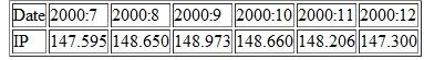
Use this AR(4) to forecast the value of Y t in January 2001 using the following values of IP for August 2000 through December 2000:
c. Worried about potential seasonal fluctuations in production, the forecaster adds Y t- 1 to the autoregression. The estimated coefficient on Y t-12 is -0.054 with a standard error of 0.053. Is this coefficient statistically significant
d. Worried about a potential break, she computes a QLR test (with 15% trimming) on the constant and AR coefficients in the AR(4) model. The resulting QLR statistic was 3.45. Is there evidence of a break Explain.
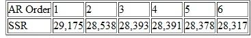
e. Worried that she might have included too few or too many lags in the model, the forecaster estimates AR( p ) models for p = 1,... ,6 over the same sample period. The sum of squared residuals from each of these estimated models is shown in the table. Use the BIC to estimate the number of lags that should be included in the autoregression. Do the results differ if you use the AIC