A Visual Approach to SPSS for Windows 2nd Edition by Leonard Stern

Exercise 1

The file Bodytemp.sav was created in Exercise 1. The file contains values of body temperature for randomly selected males and females.
1. Form a frequency distribution of the variable bodytemp. Include a table that shows the mean and standard deviation, kurtosis and skewness, and value of the distribution's 25 th , 50 th and 75 th percentiles. Plot the values of the variable using a histogram that has a normal distribution superimposed over it.
2. From the frequency distribution, determine the percentile rank of the body temperature 98.6 degrees.
3. Based on your output, is the distribution of the variable bodytemp approximately normal
Exercise 1
The data for this exercise are from Shoemaker (1996). The data set for this exercise is available from http://www.amstat.org/publications/jse/jse_data_archive.html The file is given the name normtemp.dat or normtemp.txt.
1. Download the article from the address shown above and save it on the desktop (or some other convenient location).
2. Read the data from your saved file into SPSS using the data wizard.
3. Create variable names and labels for the variables. The table below shows the correspondence between the order in which the variables are listed and their identity. Use the text in the column labeled Description as the variable label.

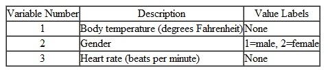
4. Make value labels for the variable named Gender.
5. If the first line of data in the SPSS Statistics Data Editor is blank, remove the case.
6. Change the number of decimal places for variable 1 to 1, and for variable 3 to 0.
7. Save the data file to your desktop (or some other convenient location) as an SPSS file named bodytemp.sav.