A Visual Approach to SPSS for Windows 2nd Edition by Leonard Stern

Exercise 5

The data file HappyMarried.sav contains responses of 1200 randomly selected adults to two questions asked in the General Social Survey given in 2004: "Are you currently--married, widowed, divorced, separated, or have you never been married " and "Taken all together, how would you say things are these days--would you say that you are very happy, pretty happy, or not too happy " Responses to the questions are coded in the data file as shown in the table below:
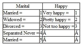Determine whether the variables Marital and Happy are significantly related.

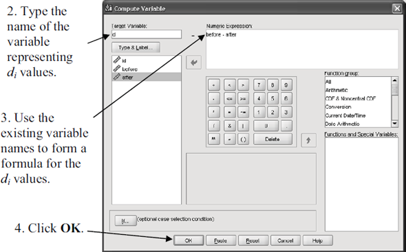
The difference scores can then be analyzed using the Explore procedure to check of the assumption of normality. Results of the t -test can be reported as follows:
The effect of the diet on weight loss of 20 randomly selected adults was examined by weighing each participant one week before the diet ( M = 149.93, SD = 15.43) and one week after the diet ( M = 146.53, SD = 14.96). Difference scores were computed by subtracting each participant's weight after the diet from his/her weight before the diet. An informal analysis of the distribution of these difference scores using a histogram and normal Q-Q plot revealed no serious threats to the assumption of normality. A t -test for paired samples showed the difference between the means was significant, t (19) = 5.13, p.001. The effect size as measure by d was 1.15, a value corresponding to a large treatment effect. Thus, the diet had a large, reliable effect on weight loss.