Ecology 7th Edition by Manuel Molles

Exercise 19

Ecologists often ask questions about observed frequencies of individuals in a population relative to some theoretical or expected frequencies. For example, an ecologist studying the nesting habits of Darwin's finches may be interested in the frequency at which finches nest in alternative nest sites relative to the availability of the alternative nest sites in the environment. Another ecologist studying the habitat association of a plant may be interested in its relative frequencies in sandy, loamy, or clay soils. An ecologist studying the mating behavior of some species may want to determine whether alternative male phenotypes (males with different physical and/or behavioral characteristics) occur at different frequencies in the population.
A common method to test hypotheses concerning the relationship between observed and hypothesized frequencies is the chi-square ( x 2 ) "goodness of fit" test. This test is used to judge how well an observed distribution of frequencies matches one "expected" from a particular hypothesis. Let's explore this test using the frequency of alternative male phenotypes in a population of side-blotched lizards, Uta stansburiana. Barry Sinervo (Sinervo and Lively 1996) found that males in populations of side-blotched lizards of the coastal range of central California include three male phenotypes: very aggressive orange-throat males, moderately aggressive blue-throat males, and sneaker yellow-throat males. Sinervo and his colleagues also found that these three male phenotypes vary in their frequencies over time. Let's consider the following hypothetical table of data from a population and test the hypothesis that the three male phenotypes are present in equal frequencies in the population.

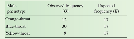
Before proceeding with our test, let's reflect on what we are doing. We would like to know if there are differences in the frequencies of male phenotypes in this population of sideblotched lizards. So, we went out and obtained a sample of 51 males from the population. This sample included 12 orangethroat males, 30 blue-throat males, and 9 yellow-throat males. Our sample is an estimate of the actual frequencies of the three phenotypes in the larger population that we are studying. Because our hypothesis is that there are no differences in frequencies among the male phenotypes, the "expected" frequencies, in the third column of our table, are equal

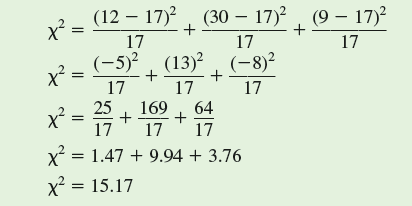
Let's use the chi-square ( x 2 ) "goodness of fit" test to determine how well our observed frequency distribution matches the expected frequency distribution. The value of x 2 is calculated as follows:

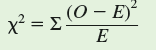
In this equation, O is the observed frequency of a particular phenotype and E is the expected frequency. If we enter the values from the table, we get the following:

The next step in the chi-square test is to determine whether the difference between observed and expected values, as indexed by our calculated x 2 is "significant." We determine significance by comparing our calculated value of x 2 with a table of x 2 values, which are included in most statistics textbooks. In order to find the appropriate, or critical, value of x 2 from such a table, we need to know two things. First, we need to choose a level of significance, which, as we saw in chapter 10 (p. 236), is generally P 0.05. Second, we need to know the "degrees of freedom," which, in this case, is the number of male phenotypes (3), or n minus 1.


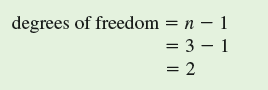
What does "degrees of freedom" mean It is the number of values we can pick freely without being constrained by other values within a set. In the case of the frequency of three male phenotypes, given a particular sample size, once we know the frequencies of two of the phenotypes, we automatically know the third. For instance, with a sample of 51 lizards, once we determine that there are 12 orange-throat males and 30 bluethroat males in our sample, the frequency of yellow-throat males is constrained to be 9. So, in this sample of three male phenotypes, there are two degrees of freedom.
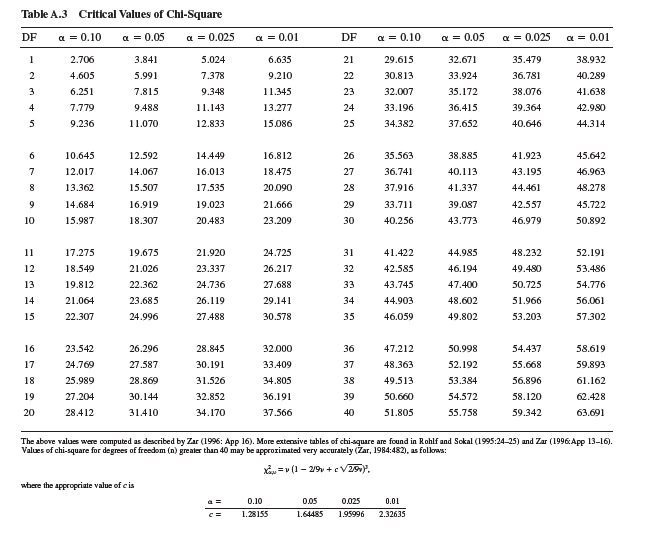
In a table of critical values of chi-square (see p. 532), you will find that for a significance level of P = 0.05 and 2 degrees of freedom, the critical x 2 value is 5.991. Since our calculated value of x 2 (15.17) is greater than 5.991, we reject the hypothesis that the three male phenotypes are present in equal frequencies in our study population. In other words, we have evidence of significant differences in frequency among the three phenotypes. And, we can attach a probability statement to this conclusion, which is P 0.05.

Suppose Sinervo and Lively study another population of side-blotched lizards in which there are five male phenotypes. If they did a "goodness of fit" analysis to test for an equal distribution of males among phenotypes in this population, what would be the degrees of freedom for their test and what would be the critical value of x 2 for P = 0.05