Ecology 7th Edition by Manuel Molles

Exercise 2

Suppose you are studying the life history of three species of herbaceous plants in a desert landscape. As part of that study, you are interested in determining the pattern of distribution of individuals in each population. Your hypothesis states that the individuals in each population are randomly distributed across the landscape. Your alternative hypotheses propose that individuals are either clumped or uniformly distributed. In chapter 9, we reviewed a study that suggested very different patterns of distribution in three plant populations (see p. 209). In that example, the sample means and sample variances of the three hypothetical populations of plant species A, B, and C were as follows:

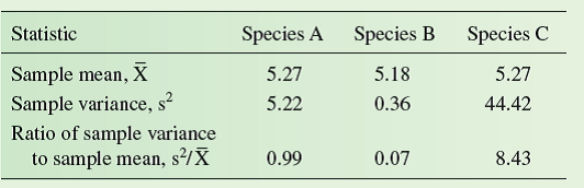
Also in chapter 9, we reviewed how in a randomly distributed population, variance/mean = 1, while in a regularly distributed population, variance/mean 1, and in a clumped population, variance/mean 1. Given these relationships, the
ratios in the above table suggest that species A has a random distribution, species B has a regular distribution, and species C has a clumped distribution. However, since the values in the table are statistical estimates of the true variance/mean ratios in the study populations we need to do a statistical test to determine the significance of our results.
The first step in our test is to establish a hypothesis. In each case, our hypothesis states that the variance/mean ratio of the population equals 1. We next need to determine a significance level, which we have seen (p. 236) is generally P 0.05. We can use a chi-square test to determine whether a sample variance/ sample mean ratio is significantly different from 1 as follows:

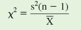
Here, N₂ 1 is the degrees of freedom, which is the sample size minus 1. In the case of our plant study, the sample size, n, is the number of sample quadrats studied for each population, which was 11 (see p. 209).
For our sample of the species A population, the calculation is:

How do we determine if these values of chi-square are statistically significant at P 0.05 Here, we need to consider whether the
ratios are significantly greater than 1, or significantly less than 1. So, in contrast to the situation that we analyzed in chapter 11, we will compare our chi-square values to two critical values, one small and one large.
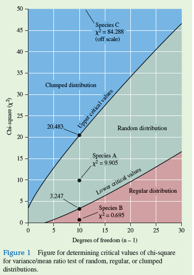
The situation we are considering is pictured in figure 1. With degrees of freedom of 10 (11 - 1 = 10), the critical values of chi-square are x 2 = 3.247 and x 2 = 20.483. As shown in figure 1 , these values of chi-square fall on the lines that form the boundaries of the area shaded green. For values of chi-square within the green area, we accept the hypothesis that the variance/mean ratio in the population equals 1, and that the population has a random distribution. Values of chi-square in the blue zone indicate a clumped distribution, while values in the red zone indicate a regular distribution. Returning to the populations of species A, B, and C, we accept the hypothesis that the variance/mean ratio of species A (X 2 = 9.905) does not differ significantly from 1, and therefore, we conclude that it has a random distribution. Meanwhile, because the value of chi-square for species B (X 2 =0695) is less than the critical value of 3.247, we reject the hypothesis that the variance/ mean ratio for species B equals 1, and conclude that it has a regular distribution. Using similar logic, we conclude that species C (X 2 = 84.288) has a cluped distribution.

Do the results of the chi-square test for species B show beyond a doubt that its population has a regular distribution