Ecology 7th Edition by Manuel Molles

Exercise 20

The question we consider now is how to represent variation in samples drawn from populations in which measurements or observations do not have normal distributions. When analyzing normally distributed measurements, depending on our purpose, we can estimate and represent variation using the range, variance, standard deviation, standard error, or 95% confidence interval. However, most of these indices of variation are not appropriate for non-normal distributions.
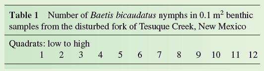
To help us consider how to represent variation when analyzing non-normal distributions, let's return to a sample of mayfly nymphs that we considered in Investigating the Evidence 3 of chapter 3 ( table 1 ). Suppose you are studying the recovery of this population following disturbance by a flash flood. The sample was taken from the south fork of Tesuque Creek, New Mexico, a high mountain stream of the southern Rocky Mountains. This fork had flooded 1 year before the sample was taken.



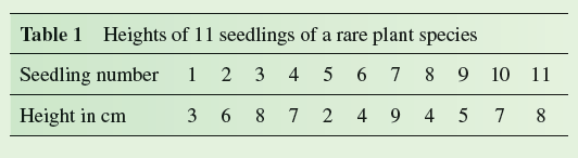
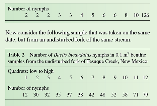
In Investigating the Evidence 3, we determined the median density of B. bicaudatus in the disturbed fork ( table 1 ) as: Sample median = 4 + 5 = 4.5 B. bicaudatus per 0.1 m 2 quadrat The median density of B. bicaudatus in the undisturbed fork ( table 2) is: Sample median = 38 + 42
= 40 B. bicaudatus per 0.1 m 2 quadrat
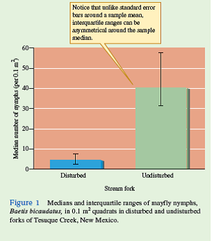
The median indicates that the density of B. bicaudatus is 10 times higher in the undisturbed fork. Now, how can we represent the variation around these medians One common method to represent variation in cases such as these is to divide the samples into four equal parts, called quartiles, and use the range of measurements between the upper bound of the lowest quartile and the lower bound of the highest quartile. This representation of variation in a sample is called the interquartile range.
In table 3 , the data in tables 1 and 2 have been divided into quartiles with different colors:

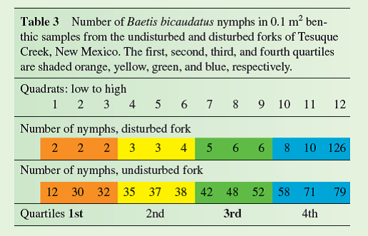
Notice that the interquartile range for the undisturbed fork is from 32 to 58; for the disturbed fork, the interquartile range is 2 to 8. Notice that 50% of the quadrat counts in each sample fall within this range. The medians and interquartile ranges for each of the populations are plotted in figure 1 , which shows that they do not overlap. However, is there a statistically significant difference in density in the two stream forks To answer that question, we will need a method for comparing samples that does not assume a normal distribution. We will make that comparison in chapter 21.

Why can an interquartile range around a median, even when sample sizes are large, be asymmetrical