Introductory Econometrics 4th Edition by Jeffrey Wooldridge

Exercise 2

A partial adjustment model is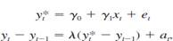
where yt* is the desired or optimal level of y, and yt is the actual (observed) level. For example, yt* is the desired growth in firm inventories, and xt is growth in firm sales. The parameter 1 measures the effect of xt on yt*. The second equation describes how the actual y adjusts depending on the relationship between the desired y in time t and the actual y in time t - 1. The parameter measures the speed of adjustment and satisfies 0 1.
(i) Plug the first equation for yt* into the second equation and show that we can write In particular, find the j in terms of the j and and find ut in terms of et and at.
Therefore, the partial adjustment model leads to a model with a lagged dependent variable and a contemporaneous x.