Deck 7: Scatterplots, Association, and Correlation
Full screen (f)
Question
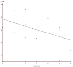
A San Jose State student collects data from 20 students. He compares the number of classes a student is enrolled in to their GPA. Here are the results of the regression analysis. The conditions for inference are satisfied.
Simple linear regression results:
Dependent Variable: GPA
Sample size: 20
Simple linear regression results: Dependent Variable: GPA Sample size: 20
R-sq = 0.26753742 s: 0.45747
-Is there evidence of a significant relationship between number of classes and GPA? Provide statistical justification for your answer.
Question
Poverty In a study of how the burden of poverty varies among U.S. regions, a random sample of 1000 individuals from each region of the United States recently yielded the information on poverty (based on defining the poverty level as an income below $10,400 for a family of 4 people). The data are provided in the table below. (All the conditions are satisfied - don't worry about checking them.)
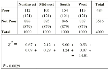
a. Write appropriate hypotheses.
b. How many degrees of freedom?
c. Suppose the expected values had not been given. Show exactly how to calculate the expected count in the first cell.
d. State your complete conclusion in context.
a. Write appropriate hypotheses.
b. How many degrees of freedom?
c. Suppose the expected values had not been given. Show exactly how to calculate the expected count in the first cell.
d. State your complete conclusion in context.
Question
Question
Question
Question
Question
Cheater? A group of curious college students decide to test the integrity of their fellow collegians. In order to see if students will cheat, when given an opportunity, they decide to use chocolately M&M's. They tell each student that a discerning palette will be able to tell the difference in flavor between and red and a yellow candy. The blindfolded subjects are given two piles of candy to test. But the experimenter turns his back so that the subject thinks that they have a window of opportunity to take a quick peak. Unbeknownst to the subjects, there is another helper who is hidden and secretly watching to see who cheats. Here is their data. 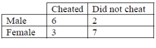
a. What is the probability that a subject cheated?
b. If a subject was a male, what are the chances that they cheated?
c. Using your answers to (a) and (b), does it appear that cheating and gender are
independent?
d. A statistics student in the group decides she wants to run a Chi-square test for independence. Why would this not be an advisable choice?
e. An argument begins. The girls are suggesting that the guys cheated more than girls; and
that this difference is larger than can be explained by chance variation. Of course, the guys insist that with a small sample size like this, anything could happen. Fortunately, a randomization machine is discovered. The 18 observations are randomly placed into the 4 categories randomly. This procedure is repeated 1000 times and the number of male
cheaters is counted each time. A graph is below. What does this graph tell you about the claims of the two groups?
Question
A sports analyst was interested in finding out how well a football team's winning percentage (stated as a proportion) can be predicted based upon points scored and points allowed. She selects a random sample of 15 football teams. Each team played 10 games. She decided to use the point differential, points scored minus points allowed as the predictor variable. The data are shown in the table below, and regression output is given afterward.
Is there evidence of an association between Point Differential and Winning Percentage? Test an appropriate hypothesis and state your conclusion in the proper context.
Is there evidence of an association between Point Differential and Winning Percentage? Test an appropriate hypothesis and state your conclusion in the proper context.
Question
Suppose you were asked to analyze each of the situations described below. (NOTE: DO NOT DO THESE PROBLEMS!) For each, indicate which inference procedure you would use (from the list), the test statistic (z, t, or ç₂ ), and, if t or ç₂ , the number of degrees of freedom. 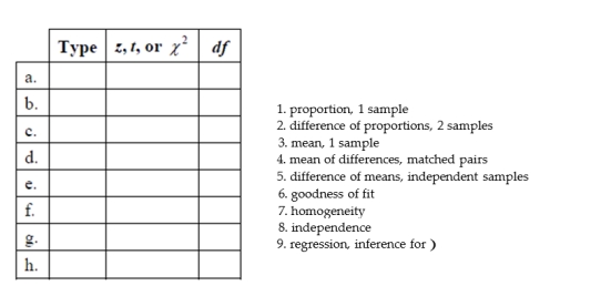
a. Doctors offer small candies to sixty teenagers, recording the number of candies consumed by each. One hour later they test the blood sugar level for each person. Is there any evidence that high blood sugar levels in teenagers are related to the amount of candy eaten?
b. Which takes less time to travel to work -- car or train? We select a random sample of 45 businessmen and compare their travel time to work for both types of commute.
c. An orthodontist wonders if soda in the diet may be a factor in loose cement on children's braces. She checks the cement bonds of 40 randomly selected patients who do not drink soda, and 40 patients who do drink soda.
d. Forty people complaining of allergies take an antihistamine. They report that their discomfort subsided in an average of 18 minutes; the standard deviation was 4 minutes. The manufacturer wants a 95% confidence interval for the "relief time".
e. A health professional selected a random sample of 100 patients from each of four major hospital emergency rooms to see if the primary reasons for emergency room visits are similar in all four major hospitals. The primary reasons were categorized as accident, illegal activity, illness, or other.
f. A policeman believes that more than 40% of older drivers speed on highways, but a confidential survey found that 49 of 88 randomly selected older drivers admitted speeding on highways at least once. Is this strong evidence that the policeman was wrong?
g. According to United Nations Population Division, the age distribution of the Commonwealth of Australia is: 21% less than 15 years of age, 67% between 15 and 65 years of age, and 12% are over 65 years old. A random sample of 210 residents of Canberra revealed 40 were less than 15 years of age, 145 were between 15 and 65 years of age, and 25 were over 65 years old. Are the ages of Canberra residents unusual in any way?
h. Among a random sample of college-age students, 6% of the 473 men said they had been adopted, compared to only 4% of the 552 women. Does this indicate a significant difference between adoption rates of males and females in college-age students?
Question
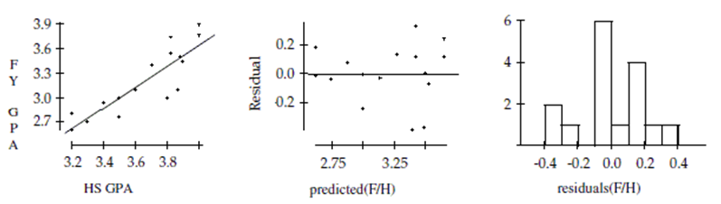
A college admissions counselor was interested in finding out how well high school grade point averages (HS GPA) predict first-year college GPAs (FY GPA). A random sample of data from first-year students was reviewed to obtain high school and first-year college GPAs. The data are shown below:
Dependent variable is: FY GPA
No Selector
squared squared (adjusted)
with degrees of freedom
-Is there evidence of an association between high school and first-year college GPAs? Test an appropriate hypothesis and state your conclusion in the proper context.
Dependent variable is: FY GPA
No Selector
squared squared (adjusted)
with degrees of freedom
-Is there evidence of an association between high school and first-year college GPAs? Test an appropriate hypothesis and state your conclusion in the proper context.
Question
Question
Question
A college admissions counselor was interested in finding out how well high school grade point averages (HS GPA) predict first-year college GPAs (FY GPA). A random sample of data from first-year students was reviewed to obtain high school and first-year college GPAs. The data are shown below:
Dependent variable is: FY GPA
No Selector
squared squared (adjusted)
with degrees of freedom
-Create and interpret a 95% confidence interval for the slope of the regression line.
Dependent variable is: FY GPA
No Selector
squared squared (adjusted)
with degrees of freedom
-Create and interpret a 95% confidence interval for the slope of the regression line.
Question
Question
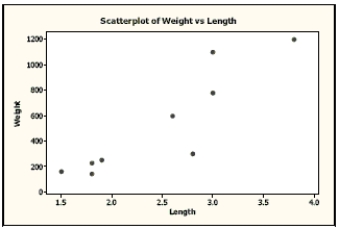
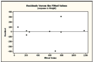
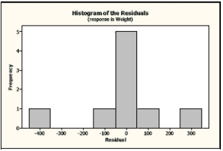
Carnivores A random sample of some of the heaviest carnivores on Earth was reviewed to determine if there is an association between the length (in meters) and weight (in kilograms) of these carnivores. Here are the scatterplot, the residuals plot, a histogram of the residuals, and the regression analysis of the data. Use this information to analyze the association between the length and weight of these carnivores.
The regression equation is
Weight Length
a. Is there an association? Write appropriate hypotheses.
b. Are the assumptions for regression satisfied? Explain.
c. What do you conclude?
d. Create a 98% confidence interval for the true slope.
e. Explain in context what your interval means.
The regression equation is
Weight Length
a. Is there an association? Write appropriate hypotheses.
b. Are the assumptions for regression satisfied? Explain.
c. What do you conclude?
d. Create a 98% confidence interval for the true slope.
e. Explain in context what your interval means.
Question
Question
Question
Of the 23 first year male students at State U. admitted from Jim Thorpe High School, 8 were offered baseball scholarships and 7 were offered football scholarships. The University admissions committee looked at the students' composite ACT scores (shown in table), wondering if the University was lowering their standards for athletes. Assuming that this group of students is representative of all admitted students, what do you think?
Boxplots:
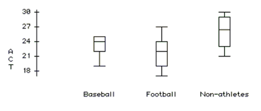
Normal Probability Plot:
-Test an appropriate hypothesis and state your conclusion
Boxplots:
Normal Probability Plot:
-Test an appropriate hypothesis and state your conclusion
Question
Question
Question
Question
A San Jose State student collects data from 20 students. He compares the number of classes a student is enrolled in to their GPA. Here are the results of the regression analysis. The conditions for inference are satisfied.
Simple linear regression results: Dependent Variable: GPA Sample size: 20
R-sq = 0.26753742 s: 0.45747
-What is the correlation coefficient for this relationship? Interpret this result in context.
Simple linear regression results: Dependent Variable: GPA Sample size: 20
R-sq = 0.26753742 s: 0.45747
-What is the correlation coefficient for this relationship? Interpret this result in context.
Question
Question
Question
A high school counselor was interested in finding out how well student grade point averages (GPA) predict ACT scores.
A sample of the senior class data was reviewed to obtain GPA and ACT scores. The data are shown in the table, and regression output is given below.
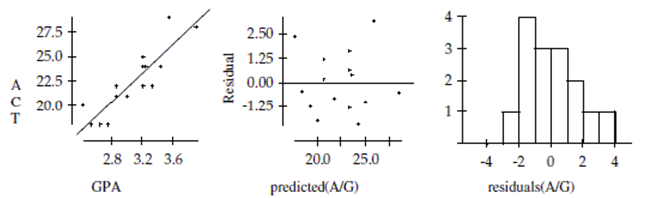
Dependent variable is:
No Selector
squared squared (adjusted)
with degrees of freedom
-Is there evidence of an association between GPA and ACT score? Test an appropriate hypothesis and state your conclusion in the proper context.
A sample of the senior class data was reviewed to obtain GPA and ACT scores. The data are shown in the table, and regression output is given below.
Dependent variable is:
No Selector
squared squared (adjusted)
with degrees of freedom
-Is there evidence of an association between GPA and ACT score? Test an appropriate hypothesis and state your conclusion in the proper context.
Question
Question
Question
Height and weight Last fall, as our first example of correlation, we looked at the heights and weights of some AP* Statistics students. Here are the scatterplot, the residuals plot, a histogram of the residuals, and the regression analysis for the data we collected from the males. Use this information to analyze the association between heights and weights of teenage boys.
Dependent variable is:WT(lb)
squared
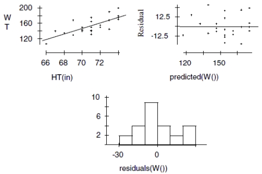
a. Is there an association? Write appropriate hypotheses. b. Are the assumptions for regression satisfied? Explain. c. What do you conclude?
d. Create a 95% confidence interval for the true slope.
e. Explain in context what your interval means.
Dependent variable is:WT(lb)
squared
a. Is there an association? Write appropriate hypotheses. b. Are the assumptions for regression satisfied? Explain. c. What do you conclude?
d. Create a 95% confidence interval for the true slope.
e. Explain in context what your interval means.
Question
Question
A San Jose State student collects data from 20 students. He compares the number of classes a student is enrolled in to their GPA. Here are the results of the regression analysis. The conditions for inference are satisfied.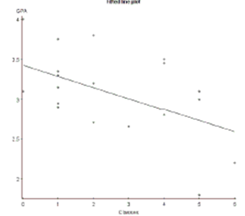
Simple linear regression results: Dependent Variable: GPA Sample size: 20
R-sq = 0.26753742 s: 0.45747
-Find and interpret a 95% confidence interval for the slope of the regression equation.
Simple linear regression results: Dependent Variable: GPA Sample size: 20
R-sq = 0.26753742 s: 0.45747
-Find and interpret a 95% confidence interval for the slope of the regression equation.
Question
Question
Of the 23 first year male students at State U. admitted from Jim Thorpe High School, 8 were offered baseball scholarships and 7 were offered football scholarships. The University admissions committee looked at the students' composite ACT scores (shown in table), wondering if the University was lowering their standards for athletes. Assuming that this group of students is representative of all admitted students, what do you think?
Boxplots:
Normal Probability Plot:
-Are the two sports teams mean ACT scores different?
Boxplots:
Normal Probability Plot:
-Are the two sports teams mean ACT scores different?
Question
Question
It's common for a movie's ticket sales to open high for the first couple of weeks, then gradually taper off as time passes. Hoping to be able to better understand how quickly sales decline, an industry analyst keeps track of box office revenues for a new film over its first 20 weeks. What inference method might provide useful insight?
Question
Question
Question
Question
Question
Cloning A random sample of 800 adults was asked the following question: "Do you think
current laws concerning the use of cloning for medical research are too strict, too lenient, or about
right?" The pollsters also classified the respondents with respect to highest education level attained: high school, 2-year college degree, 4-year degree, or advanced degree. We wish to know if attitudes on cloning are related to education level. (All the conditions are satisfied - don't worry about checking them.)
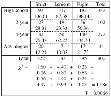
a. Write appropriate hypotheses.
b. Suppose the expected counts had not been given. Show how to calculate the expected count in the first cell (106.01).
c. How many degrees of freedom?
d. State your complete conclusion in context.
current laws concerning the use of cloning for medical research are too strict, too lenient, or about
right?" The pollsters also classified the respondents with respect to highest education level attained: high school, 2-year college degree, 4-year degree, or advanced degree. We wish to know if attitudes on cloning are related to education level. (All the conditions are satisfied - don't worry about checking them.)
a. Write appropriate hypotheses.
b. Suppose the expected counts had not been given. Show how to calculate the expected count in the first cell (106.01).
c. How many degrees of freedom?
d. State your complete conclusion in context.
Question

Unlock Deck
Sign up to unlock the cards in this deck!
Unlock Deck
Unlock Deck
1/40
Play
Full screen (f)
Deck 7: Scatterplots, Association, and Correlation
1
A San Jose State student collects data from 20 students. He compares the number of classes a student is enrolled in to their GPA. Here are the results of the regression analysis. The conditions for inference are satisfied.
Simple linear regression results:
Dependent Variable: GPA
Sample size: 20
Simple linear regression results: Dependent Variable: GPA Sample size: 20
R-sq = 0.26753742 s: 0.45747
-Is there evidence of a significant relationship between number of classes and GPA? Provide statistical justification for your answer.
H0: ) = 0 There is no evidence of a linear relationship between number of classes and GPA.
HA: ) × 0 There is evidence of a linear relationship between number of classes and
GPA.
The conditions for inference have been met. t = -2.56; df = 18; p-value = 0.0195; a = 0.05
With a p-value of 1.95% < 5%, I reject H?. We have statistically significantly evidence that there is a linear relationship between number of classes and GPA.
2
Poverty In a study of how the burden of poverty varies among U.S. regions, a random sample of 1000 individuals from each region of the United States recently yielded the information on poverty (based on defining the poverty level as an income below $10,400 for a family of 4 people). The data are provided in the table below. (All the conditions are satisfied - don't worry about checking them.)
a. Write appropriate hypotheses.
b. How many degrees of freedom?
c. Suppose the expected values had not been given. Show exactly how to calculate the expected count in the first cell.
d. State your complete conclusion in context.
a. Write appropriate hypotheses.
b. How many degrees of freedom?
c. Suppose the expected values had not been given. Show exactly how to calculate the expected count in the first cell.
d. State your complete conclusion in context.
a. : Poverty percentages are the same for the geographic regions in the Unites States.
: Poverty percentages differ by geographic region in the United States.
b. degrees of freedom
c.
d. Since the -value of is so low, there is strong evidence that poverty percentages differ by geographic location in the United States. We will reject the null hypothesis and conclude that poverty is associated with geographic location in the United States. Specifically, the South contains a greater proportion of people below the poverty level than expected.
3
Suppose that after the study described in #5 we want to see if there's evidence that the exercise program's effectiveness in lowering blood pressure depends on how high the person's initial blood pressure was. We should do a
A) ç2 test of independence
B) ç2 goodness-of-fit test
C) matched pairs t-test
D) linear regression t-test
E) 2-sample t-test
A) ç2 test of independence
B) ç2 goodness-of-fit test
C) matched pairs t-test
D) linear regression t-test
E) 2-sample t-test
linear regression t-test
4
A flower pot manufacturer is testing his clay pots to ensure that the thickness of the sides are made to proper specifications. The sides are designed to be 4 mm thick. In a random sample of 25 pots, it is found that the average thickness if 4.3 mm. Does this provide statistically significant evidence that the manufacturing process is out of alignment?
Unlock Deck
Unlock for access to all 40 flashcards in this deck.
Unlock Deck
k this deck
5
College admissions According to information from a college admissions office, 62% of the students there attended public high schools, 26% attended private high schools, 2% were home schooled, and the remaining students attended schools in other countries. Among this college's Honors Graduates last year there were 47 who came from public schools, 29 from private schools, 4 who had been home schooled, and 4 students from abroad. Is there any evidence that one type of high school might better equip students to attain high academic honors at this college? Test an appropriate hypothesis and state your conclusion.
Unlock Deck
Unlock for access to all 40 flashcards in this deck.
Unlock Deck
k this deck
6
Peanut M&Ms According to the Mars Candy Company, peanut M&M's are 12% brown,
15% yellow, 12% red, 23% blue, 23% orange, and 15% green. On a Saturday when you have
run out of statistics homework, you decide to test this claim. You purchase a medium bag
of peanut M&M's and find 39 browns, 44 yellows, 36 red, 78 blue, 73 orange, and 48 greens. Test an appropriate hypothesis and state your conclusion.
Unlock Deck
Unlock for access to all 40 flashcards in this deck.
Unlock Deck
k this deck
7
Cheater? A group of curious college students decide to test the integrity of their fellow collegians. In order to see if students will cheat, when given an opportunity, they decide to use chocolately M&M's. They tell each student that a discerning palette will be able to tell the difference in flavor between and red and a yellow candy. The blindfolded subjects are given two piles of candy to test. But the experimenter turns his back so that the subject thinks that they have a window of opportunity to take a quick peak. Unbeknownst to the subjects, there is another helper who is hidden and secretly watching to see who cheats. Here is their data.
a. What is the probability that a subject cheated?
b. If a subject was a male, what are the chances that they cheated?
c. Using your answers to (a) and (b), does it appear that cheating and gender are
independent?
d. A statistics student in the group decides she wants to run a Chi-square test for independence. Why would this not be an advisable choice?
e. An argument begins. The girls are suggesting that the guys cheated more than girls; and
that this difference is larger than can be explained by chance variation. Of course, the guys insist that with a small sample size like this, anything could happen. Fortunately, a randomization machine is discovered. The 18 observations are randomly placed into the 4 categories randomly. This procedure is repeated 1000 times and the number of male
cheaters is counted each time. A graph is below. What does this graph tell you about the claims of the two groups?
Unlock Deck
Unlock for access to all 40 flashcards in this deck.
Unlock Deck
k this deck
8
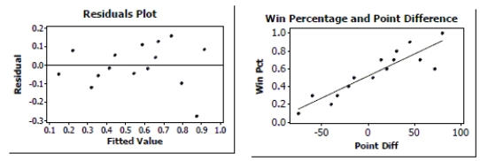
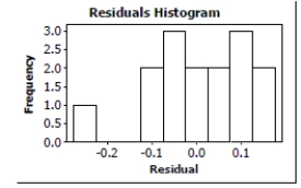
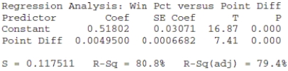
A sports analyst was interested in finding out how well a football team's winning percentage (stated as a proportion) can be predicted based upon points scored and points allowed. She selects a random sample of 15 football teams. Each team played 10 games. She decided to use the point differential, points scored minus points allowed as the predictor variable. The data are shown in the table below, and regression output is given afterward.
Is there evidence of an association between Point Differential and Winning Percentage? Test an appropriate hypothesis and state your conclusion in the proper context.
Is there evidence of an association between Point Differential and Winning Percentage? Test an appropriate hypothesis and state your conclusion in the proper context.
Unlock Deck
Unlock for access to all 40 flashcards in this deck.
Unlock Deck
k this deck
9
Suppose you were asked to analyze each of the situations described below. (NOTE: DO NOT DO THESE PROBLEMS!) For each, indicate which inference procedure you would use (from the list), the test statistic (z, t, or ç₂ ), and, if t or ç₂ , the number of degrees of freedom.
a. Doctors offer small candies to sixty teenagers, recording the number of candies consumed by each. One hour later they test the blood sugar level for each person. Is there any evidence that high blood sugar levels in teenagers are related to the amount of candy eaten?
b. Which takes less time to travel to work -- car or train? We select a random sample of 45 businessmen and compare their travel time to work for both types of commute.
c. An orthodontist wonders if soda in the diet may be a factor in loose cement on children's braces. She checks the cement bonds of 40 randomly selected patients who do not drink soda, and 40 patients who do drink soda.
d. Forty people complaining of allergies take an antihistamine. They report that their discomfort subsided in an average of 18 minutes; the standard deviation was 4 minutes. The manufacturer wants a 95% confidence interval for the "relief time".
e. A health professional selected a random sample of 100 patients from each of four major hospital emergency rooms to see if the primary reasons for emergency room visits are similar in all four major hospitals. The primary reasons were categorized as accident, illegal activity, illness, or other.
f. A policeman believes that more than 40% of older drivers speed on highways, but a confidential survey found that 49 of 88 randomly selected older drivers admitted speeding on highways at least once. Is this strong evidence that the policeman was wrong?
g. According to United Nations Population Division, the age distribution of the Commonwealth of Australia is: 21% less than 15 years of age, 67% between 15 and 65 years of age, and 12% are over 65 years old. A random sample of 210 residents of Canberra revealed 40 were less than 15 years of age, 145 were between 15 and 65 years of age, and 25 were over 65 years old. Are the ages of Canberra residents unusual in any way?
h. Among a random sample of college-age students, 6% of the 473 men said they had been adopted, compared to only 4% of the 552 women. Does this indicate a significant difference between adoption rates of males and females in college-age students?
Unlock Deck
Unlock for access to all 40 flashcards in this deck.
Unlock Deck
k this deck
10
A college admissions counselor was interested in finding out how well high school grade point averages (HS GPA) predict first-year college GPAs (FY GPA). A random sample of data from first-year students was reviewed to obtain high school and first-year college GPAs. The data are shown below:
Dependent variable is: FY GPA
No Selector
squared squared (adjusted)
with degrees of freedom
-Is there evidence of an association between high school and first-year college GPAs? Test an appropriate hypothesis and state your conclusion in the proper context.
Dependent variable is: FY GPA
No Selector
squared squared (adjusted)
with degrees of freedom
-Is there evidence of an association between high school and first-year college GPAs? Test an appropriate hypothesis and state your conclusion in the proper context.
Unlock Deck
Unlock for access to all 40 flashcards in this deck.
Unlock Deck
k this deck
11
Height and weight Is the height of a man related to his weight? The regression analysis from a sample of 26 men is shown. (Show work. Don't write hypotheses. Assume the assumptions for inference were satisfied.)
a. How many degrees of freedom?
b. What is the value of the t statistic?
c. What is the P-value?
d. State your conclusion in context.
a. How many degrees of freedom?
b. What is the value of the t statistic?
c. What is the P-value?
d. State your conclusion in context.
Unlock Deck
Unlock for access to all 40 flashcards in this deck.
Unlock Deck
k this deck
12
For the scenario described below, simply name the procedure that is appropriate to answer the question. For example,
1-proportion z-interval or chi-square goodness of fit test. Do NOT carry out the procedure.
-A national marketing campaign is conducted to improve the name-brand recognition with potential customers. The company sells household products, primarily to the female head of the household. The current market analysis shows that 23% of their customer base recognizes the name of their product. When the marketing campaign is finished, 135
people out of 500 randomly polled recognize the brand name. Does this provide statistically significant evidence that there has been an increase in name-brand recognition?
Unlock Deck
Unlock for access to all 40 flashcards in this deck.
Unlock Deck
k this deck
13
A college admissions counselor was interested in finding out how well high school grade point averages (HS GPA) predict first-year college GPAs (FY GPA). A random sample of data from first-year students was reviewed to obtain high school and first-year college GPAs. The data are shown below:
Dependent variable is: FY GPA
No Selector
squared squared (adjusted)
with degrees of freedom
-Create and interpret a 95% confidence interval for the slope of the regression line.
Dependent variable is: FY GPA
No Selector
squared squared (adjusted)
with degrees of freedom
-Create and interpret a 95% confidence interval for the slope of the regression line.
Unlock Deck
Unlock for access to all 40 flashcards in this deck.
Unlock Deck
k this deck
14
As part of a survey, students in a large statistics class were asked whether or not they ate breakfast that morning. The data appears in the following table:
Is there evidence that eating breakfast is independent of the student's sex? Test an appropriate hypothesis. Give statistical evidence to support your conclusion.
Is there evidence that eating breakfast is independent of the student's sex? Test an appropriate hypothesis. Give statistical evidence to support your conclusion.
Unlock Deck
Unlock for access to all 40 flashcards in this deck.
Unlock Deck
k this deck
15
Carnivores A random sample of some of the heaviest carnivores on Earth was reviewed to determine if there is an association between the length (in meters) and weight (in kilograms) of these carnivores. Here are the scatterplot, the residuals plot, a histogram of the residuals, and the regression analysis of the data. Use this information to analyze the association between the length and weight of these carnivores.
The regression equation is
Weight Length
a. Is there an association? Write appropriate hypotheses.
b. Are the assumptions for regression satisfied? Explain.
c. What do you conclude?
d. Create a 98% confidence interval for the true slope.
e. Explain in context what your interval means.
The regression equation is
Weight Length
a. Is there an association? Write appropriate hypotheses.
b. Are the assumptions for regression satisfied? Explain.
c. What do you conclude?
d. Create a 98% confidence interval for the true slope.
e. Explain in context what your interval means.
Unlock Deck
Unlock for access to all 40 flashcards in this deck.
Unlock Deck
k this deck
16
Voter registration A random sample of 337 college students was asked whether or not they were registered to vote. We wonder if there is an association between a student's sex and whether the student is registered to vote. The data are provided in the table below
(expected counts are in parentheses). (All the conditions are satisfied - don't worry about checking them.)
a. Write appropriate hypotheses.
b. Suppose the expected values had not been given. Show exactly how to calculate the expected number of men who are registered to vote.
c. Show how to calculate the component of ç? for the first cell. d. How many degrees of freedom are there?
e. Find the P-value for this test.
f. State your complete conclusion in context.
Unlock Deck
Unlock for access to all 40 flashcards in this deck.
Unlock Deck
k this deck
17
In the study "The Role of Sports as a Social Determinant for Children," student respondents in grades 4 through 6 were asked what they would most like to do at school: make good grades, be popular or be good at sports. Results delineated by type of school district are reported below.
Source: Chase, M.A and Dummer, G.M. (1992), "The Role of Sports as a Social Determinant for
Children," Research Quarterly for Exercise and Sport, 63, 418-424.
Is there evidence that type of school district and personal school goals are independent? Test an appropriate hypothesis. Give Statistical evidence to support your conclusion.
Unlock Deck
Unlock for access to all 40 flashcards in this deck.
Unlock Deck
k this deck
18
Of the 23 first year male students at State U. admitted from Jim Thorpe High School, 8 were offered baseball scholarships and 7 were offered football scholarships. The University admissions committee looked at the students' composite ACT scores (shown in table), wondering if the University was lowering their standards for athletes. Assuming that this group of students is representative of all admitted students, what do you think?
Boxplots:
Normal Probability Plot:
-Test an appropriate hypothesis and state your conclusion
Boxplots:
Normal Probability Plot:
-Test an appropriate hypothesis and state your conclusion
Unlock Deck
Unlock for access to all 40 flashcards in this deck.
Unlock Deck
k this deck
19
Several volunteers engage in a special exercise program intended to lower their blood pressure. We measure each person's initial blood pressure, lead them through the exercises daily for a month, then check blood pressures again. To see if the program lowered blood pressure significantly we should do a
A) matched pairs t-test
B) ç2 test of homogeneity
C) 2-sample t-test
D) linear regression t-test
E) ç2 goodness-of-fit test
A) matched pairs t-test
B) ç2 test of homogeneity
C) 2-sample t-test
D) linear regression t-test
E) ç2 goodness-of-fit test
Unlock Deck
Unlock for access to all 40 flashcards in this deck.
Unlock Deck
k this deck
20
Wingspan A person's wingspan is the distance from fingertip to fingertip when their arms are fully extended. The longer a person's wingspan, the taller they tend to be. Regression analysis was executed on 24 individuals to see if height in inches can be used to predict wingspan (also in inches). The conditions for inference were deemed to be reasonably satisfied.
Dependent Variable: Wingspan
Sample size: 24
R-sq = 0.8026696 s: 2.1512606
a. Write the equation of the regression line. Make sure to define all the variables in your equation.
b. Interpret the slope of the regression equation in context. c. Interpret the value of s in context.
d. Find and interpret a 95% confidence interval for slope.
e. Is the relationship between wingspan and height a strong relationship? Why? Give two reasons to justify your answer.
^
Unlock Deck
Unlock for access to all 40 flashcards in this deck.
Unlock Deck
k this deck
21
a. H0: There is no association between height and weight.
HA: There is an association between height and weight.
b. The scatterplot looks straight enough, residuals are random and display consistent spread, the histogram of
residuals looks roughly unimodal and symmetric.
c. Reject H? because of the small P-value; there is strong evidence of an association between height and weight. d. 7.30 ± 2.75
e. We are 95% confident that teenage boys gain an average of between 4.55 and 10.05 pounds per inch of height.
Unlock Deck
Unlock for access to all 40 flashcards in this deck.
Unlock Deck
k this deck
22
A San Jose State student collects data from 20 students. He compares the number of classes a student is enrolled in to their GPA. Here are the results of the regression analysis. The conditions for inference are satisfied.
Simple linear regression results: Dependent Variable: GPA Sample size: 20
R-sq = 0.26753742 s: 0.45747
-What is the correlation coefficient for this relationship? Interpret this result in context.
Simple linear regression results: Dependent Variable: GPA Sample size: 20
R-sq = 0.26753742 s: 0.45747
-What is the correlation coefficient for this relationship? Interpret this result in context.
Unlock Deck
Unlock for access to all 40 flashcards in this deck.
Unlock Deck
k this deck
23
How many degrees of freedom are there for regression inference with 28 data values?
A) 54
B) 26
C) 27
D) 56
E) 28
A) 54
B) 26
C) 27
D) 56
E) 28
Unlock Deck
Unlock for access to all 40 flashcards in this deck.
Unlock Deck
k this deck
24
When two competing teams are equally matched, the probability that each team wins any game is 0.5. The NBA championship goes to the team that wins four games in a
best-of-seven series. If the teams were equally matched, the probability that the final series ends with one of the teams sweeping four straight games would be 2(0.5)4 = 0.125. Further probability calculations indicate that 25% of these series should last five games, 31.25% should last six games, and the other 31.25% should last the full seven games. The table shows the number of games it took to decide each of the last 57 NBA champs. Do you think the teams are usually equally matched? Give statistical evidence to support yourconclusion.
best-of-seven series. If the teams were equally matched, the probability that the final series ends with one of the teams sweeping four straight games would be 2(0.5)4 = 0.125. Further probability calculations indicate that 25% of these series should last five games, 31.25% should last six games, and the other 31.25% should last the full seven games. The table shows the number of games it took to decide each of the last 57 NBA champs. Do you think the teams are usually equally matched? Give statistical evidence to support yourconclusion.
Unlock Deck
Unlock for access to all 40 flashcards in this deck.
Unlock Deck
k this deck
25
A high school counselor was interested in finding out how well student grade point averages (GPA) predict ACT scores.
A sample of the senior class data was reviewed to obtain GPA and ACT scores. The data are shown in the table, and regression output is given below.
Dependent variable is:
No Selector
squared squared (adjusted)
with degrees of freedom
-Is there evidence of an association between GPA and ACT score? Test an appropriate hypothesis and state your conclusion in the proper context.
Unlock Deck
Unlock for access to all 40 flashcards in this deck.
Unlock Deck
k this deck
26
We want to know whether the categorical variables "eating breakfast" and "student's sex" are statistically independent.
H0: Eating breakfast and student's sex are independent.
HA: There is an association between eating breakfast and student's sex.
Conditions:
*Counted data: We have the counts of individuals in categories of two categorical variables.
*Randomization: We have a convenience sample of students, but no reason to suspect bias.
*Expected cell frequency: The expected values (shown in parenthesis in the table) are all greater than 5, so the condition is satisfied.
Under these conditions, the sampling distribution of the test statistic is ç2 with (r - 1)(c - 1) = (2 - 1)(2 - 1) = 1 degree of freedom, and we will perform a chi-square test of independence.
Unlock Deck
Unlock for access to all 40 flashcards in this deck.
Unlock Deck
k this deck
27
Suppose you were asked to analyze each of the situations described below. (NOTE: DO NOT DO THESE PROBLEMS!) For each, indicate which inference procedure you would use (from the list), the test statistic (z, t, or ç? ), and, if t or ç?, the number of degrees of freedom.
1. proportion, 1 sample
2. difference of proportions, 2 samples
3. mean, 1 sample
4. mean of differences, matched pairs
5. difference of means, independent samples
6. goodness of fit
7. homogeneity
8. independence
9. regression, inference for )
a. A researcher wonders if meat in the diet may be a factor in high blood pressure. She
compares the blood pressures of 40 randomly selected vegetarians, to those of 40 people who eat meat.
b. According to the American Red Cross, 45% of Americans have Type O blood, 40% Type A, 11% Type B, and 4% Type AB. Last week a blood drive at the high school collected 132 pints of blood. If 51 were Type O, 55 Type A, 17 Type B, and 9 were Type AB, was this yield unusual in any way?
c. Among a random sample of college-age drivers 5% of the 576 men said they had been ticketed for speeding during the past year, compared to only 3% of the 552 women. Does this indicate a significant difference between college males and females in terms of being ticketed for speeding?
d. Who is paid more in New York State - teachers or policemen? We select a random sample of 25 New York cities and find the starting salaries of teachers and policemen in each.
e. Researchers offer small cookies to nine nursery school children and record the number of cookies consumed by each. Forty-five minutes later they observe these children during recess, and rate each child for hyperactivity on a scale from 1 - 20. Is there any evidence that sugar contributes to hyperactivity in children?
f. 22 people complaining of indigestion take an antacid. They report that their discomfort subsided in an average of 13 minutes; the standard deviation was 4 minutes. The manufacturer wants a 95% confidence interval for the "relief time."
g. A sports fan selected a random sample of 100 games from each of the NBA, the NFL, the NHL, and Major League Baseball to see if overtimes (or extra innings) are equally likely to occur in all four sports.
h. A teacher believes that no more than 10% of high school students ever cheat on an exam, but a confidential survey found that 14 of 88 randomly selected students admitted having cheated at least once. Is this strong evidence that the teacher was wrong?
Unlock Deck
Unlock for access to all 40 flashcards in this deck.
Unlock Deck
k this deck
28
Height and weight Last fall, as our first example of correlation, we looked at the heights and weights of some AP* Statistics students. Here are the scatterplot, the residuals plot, a histogram of the residuals, and the regression analysis for the data we collected from the males. Use this information to analyze the association between heights and weights of teenage boys.
Dependent variable is:WT(lb)
squared
a. Is there an association? Write appropriate hypotheses. b. Are the assumptions for regression satisfied? Explain. c. What do you conclude?
d. Create a 95% confidence interval for the true slope.
e. Explain in context what your interval means.
Dependent variable is:WT(lb)
squared
a. Is there an association? Write appropriate hypotheses. b. Are the assumptions for regression satisfied? Explain. c. What do you conclude?
d. Create a 95% confidence interval for the true slope.
e. Explain in context what your interval means.
Unlock Deck
Unlock for access to all 40 flashcards in this deck.
Unlock Deck
k this deck
29
In a local school, vending machines offer a range of drinks from juices to sports drinks. The purchasing agent thinks each type of drink is equally favored among the students buying drinks from the machines. The recent purchasing choices from the vending machines are shown in the table.
a. Test an appropriate hypothesis to decide if the purchasing agent is correct. Give statistical evidence to support your conclusion.
b. Which type of drink impacted your decision the most? Explain what this means in the
context of the problem.
a. Test an appropriate hypothesis to decide if the purchasing agent is correct. Give statistical evidence to support your conclusion.
b. Which type of drink impacted your decision the most? Explain what this means in the
context of the problem.
Unlock Deck
Unlock for access to all 40 flashcards in this deck.
Unlock Deck
k this deck
30
A San Jose State student collects data from 20 students. He compares the number of classes a student is enrolled in to their GPA. Here are the results of the regression analysis. The conditions for inference are satisfied.
Simple linear regression results: Dependent Variable: GPA Sample size: 20
R-sq = 0.26753742 s: 0.45747
-Find and interpret a 95% confidence interval for the slope of the regression equation.
Simple linear regression results: Dependent Variable: GPA Sample size: 20
R-sq = 0.26753742 s: 0.45747
-Find and interpret a 95% confidence interval for the slope of the regression equation.
Unlock Deck
Unlock for access to all 40 flashcards in this deck.
Unlock Deck
k this deck
31
In a study on insomnia in men over the age of 65, it is found that exercise may play a role in sleep. The researchers assign a group of 100 men to exercise for a month, while another
100 volunteers are asked to abstain from most exercise. At the end of the month, the exercise group had 23 out of 100 men with difficulty in sleeping, whereas the non-exercise group had 31 out of 100. Does this provide statistically significant that exercise improves sleep for men over 65?
100 volunteers are asked to abstain from most exercise. At the end of the month, the exercise group had 23 out of 100 men with difficulty in sleeping, whereas the non-exercise group had 31 out of 100. Does this provide statistically significant that exercise improves sleep for men over 65?
Unlock Deck
Unlock for access to all 40 flashcards in this deck.
Unlock Deck
k this deck
32
Of the 23 first year male students at State U. admitted from Jim Thorpe High School, 8 were offered baseball scholarships and 7 were offered football scholarships. The University admissions committee looked at the students' composite ACT scores (shown in table), wondering if the University was lowering their standards for athletes. Assuming that this group of students is representative of all admitted students, what do you think?
Boxplots:
Normal Probability Plot:
-Are the two sports teams mean ACT scores different?
Boxplots:
Normal Probability Plot:
-Are the two sports teams mean ACT scores different?
Unlock Deck
Unlock for access to all 40 flashcards in this deck.
Unlock Deck
k this deck
33
In a campus survey, a university polls its students to see how many hours they study in an average week. Females reported an average of 16.8 hours, while males reported an average of 13.8 hours. Find a 95% confidence interval for the difference in average time spent studying by females compared to males.
Unlock Deck
Unlock for access to all 40 flashcards in this deck.
Unlock Deck
k this deck
34
It's common for a movie's ticket sales to open high for the first couple of weeks, then gradually taper off as time passes. Hoping to be able to better understand how quickly sales decline, an industry analyst keeps track of box office revenues for a new film over its first 20 weeks. What inference method might provide useful insight?
Unlock Deck
Unlock for access to all 40 flashcards in this deck.
Unlock Deck
k this deck
35
Car reliability A consumer group assigned 62 car models reliability ratings of 1 - 5 based upon repair records. They wondered if more expensive cars might be more reliable. To find out, they created the regression analysis shown. (SHOW WORK. Don't bother writing hypotheses, and you may assume the assumptions for inference were all satisfied.)
a. df = ______, t = ______, P =______
b. State your conclusion.
a. df = ______, t = ______, P =______
b. State your conclusion.
Unlock Deck
Unlock for access to all 40 flashcards in this deck.
Unlock Deck
k this deck
36
Car colors According to Ward's Communication, 19% of sports car enthusiasts prefer a red color, 16.2% silver, 14.7% black, 14.1% green, 14% white, and 22% other colors. A sample of
250 cars at a NASCAR raceway revealed 45 red cars, 42 silver cars, 34 black cars, 40 green cars, 39 white cars, and 50 other color cars. Are NASCAR color preferences typical of sports car enthusiasts? Test an appropriate hypothesis and state your conclusion.
250 cars at a NASCAR raceway revealed 45 red cars, 42 silver cars, 34 black cars, 40 green cars, 39 white cars, and 50 other color cars. Are NASCAR color preferences typical of sports car enthusiasts? Test an appropriate hypothesis and state your conclusion.
Unlock Deck
Unlock for access to all 40 flashcards in this deck.
Unlock Deck
k this deck
37
Production Workers at a large factory finish shirts with a hand sewn logo. The foreman overseeing the workers tracks the level of production. After collecting data for several months he estimates that workers complete an average of 230 shirts each day with a standard deviation of 13 shirts. He also believes that a normal model is appropriate to describe the distribution.
a) What is the probability that the workers will produce more than 250 shirts on a given
day?
b) Assuming that each day is independent, what are the chances that they will produce over 250 shirts for 3 days in a row?
a) What is the probability that the workers will produce more than 250 shirts on a given
day?
b) Assuming that each day is independent, what are the chances that they will produce over 250 shirts for 3 days in a row?
Unlock Deck
Unlock for access to all 40 flashcards in this deck.
Unlock Deck
k this deck
38
The vast majority of states and the District of Columbia have adopted the Common Core State Standards (CCSS) for math and English language arts. Do teachers support the CCSS? In March 2003, The American Federal of Teachers (AFT) asked AFT member teachers "Based on what you know about the Common Core State Standards and the expectations they set for children, do you approve or disapprove of your state's decision to adopt them?
" The following results were reported in American Educator (Volume 32, No. 2, Summer 2013, pg. 3): 27% Strongly Approve; 48% Somewhat Approve; 14% Somewhat Disapprove; 8% Strongly Approve; 3% Not Sure.
A district superintendent asked the same question to the teachers in her district to assess the level of teacher support for the CCSS within the district. She obtained the following results.
a. Test an appropriate hypothesis to ascertain if the district CCSS approval distribution matches the national AFT approval distribution.
b. Which response impacted your decision the most? Explain what this means in the context of the problem.
Unlock Deck
Unlock for access to all 40 flashcards in this deck.
Unlock Deck
k this deck
39
Cloning A random sample of 800 adults was asked the following question: "Do you think
current laws concerning the use of cloning for medical research are too strict, too lenient, or about
right?" The pollsters also classified the respondents with respect to highest education level attained: high school, 2-year college degree, 4-year degree, or advanced degree. We wish to know if attitudes on cloning are related to education level. (All the conditions are satisfied - don't worry about checking them.)
a. Write appropriate hypotheses.
b. Suppose the expected counts had not been given. Show how to calculate the expected count in the first cell (106.01).
c. How many degrees of freedom?
d. State your complete conclusion in context.
Unlock Deck
Unlock for access to all 40 flashcards in this deck.
Unlock Deck
k this deck
40
How many degrees of freedom are there for a chi-square test of independence based on a table with five rows and six columns?
A) 30
B) 4
C) 24
D) 20
E) 5
A) 30
B) 4
C) 24
D) 20
E) 5
Unlock Deck
Unlock for access to all 40 flashcards in this deck.
Unlock Deck
k this deck
Unlock Deck
Unlock for access to all 40 flashcards in this deck.


