Deck 4: Describing Bivariate Numerical Data
Full screen (f)
Question
If  , the standard deviation of y is equal to the standard deviation of the residuals.
, the standard deviation of y is equal to the standard deviation of the residuals. Question
The least squares line passes through the point  .
.
. Question
Question
Data were collected on y = price of car (in dollars) and x = age of car (in years) for each car in a sample of 60 used Toyota Camrys. A scatterplot showed a negative linear relationship between x and y. The least squares regression line was fit and the  value was computed. If
  , which of the following is a correct statement?
A)The correlation coefficient is positive, r = 0.55
B)If the least-squares line is used to predict car price based on number of miles driven, predictions should be within $0.55 of the true price.
C)There is a very strong linear relationship between car price and number of miles driven.
D)For each additional mile driven, car price increases by approximately $0.55
E)Approximately 55% of the variability in car price can be explained by the linear relationship between car price and number of miles the car has been driven.
value was computed. If , which of the following is a correct statement? A)The correlation coefficient is positive, r = 0.55
B)If the least-squares line is used to predict car price based on number of miles driven, predictions should be within $0.55 of the true price.
C)There is a very strong linear relationship between car price and number of miles driven.
D)For each additional mile driven, car price increases by approximately $0.55
E)Approximately 55% of the variability in car price can be explained by the linear relationship between car price and number of miles the car has been driven.
Question
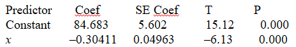
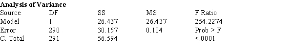
Twenty-five assembly-line workers participated in a study to investigate the relationship between experience and the amount of time required to complete an assembly task. Assembly time (in minutes) and number of months the worker had been employed on the assembly line were measured for each worker. The resulting data on y= time to complete assembly and x= number of months on the assembly line were used to produce the scatterplot and computer output below.

S= 9.79097 R-Sq = 62.0% R-Sq(adj) = 60.4%
Predict the time required to complete the assembly for an employee with 10 months of experience.
A) 81.6min
B) 90.6min
C) 110.4min
D) 120.7min
E) 150.3min
S= 9.79097 R-Sq = 62.0% R-Sq(adj) = 60.4%
Predict the time required to complete the assembly for an employee with 10 months of experience.
A) 81.6min
B) 90.6min
C) 110.4min
D) 120.7min
E) 150.3min
Question
Question
Question
Of the following, which is true of Pearson's correlation coefficient, r?
A)The value of r does not depend on the units of y and x.
B)r = 0 indicates a perfect correlation between x and y.
C)r cannot be less than 0 or greater than 1.
D)The value of r depends on which of two variables is labeled x.
E) is greater than 1.0 unless the points on a scatterplot line up exactly.
A)The value of r does not depend on the units of y and x.
B)r = 0 indicates a perfect correlation between x and y.
C)r cannot be less than 0 or greater than 1.
D)The value of r depends on which of two variables is labeled x.
E)
is greater than 1.0 unless the points on a scatterplot line up exactly. Question
Which of the following indicates the range of possible values of the coefficient of determination,  ?
?
A)
B)
C)
D)
E)
? A)
B)
C)
D)
E)
Question
Question
Data on x = the weight of a pickup truck (pounds) and y = distance (in feet) required for a truck traveling 40 miles per hour to come to a complete stop for 30 trucks was used to fit the least squares regression line  . Which of the following statements is a correct interpretation of the value 0.05 in the equation of the regression line?
A)On average, the truck weight goes up 0.05 pound for each additional foot required to stop the truck.
B)On average, the stopping distance is 0.05 foot when the truck weight is 0.
C)The correlation coefficient for this data set is 0.05
D)On average, the stopping distance goes up 0.05 foot for each 1-pound increase in truck weight.
E)Approximately 5% of the variation in the stopping distances can be explained by the linear relationship between stopping distance and truck weight.
. Which of the following statements is a correct interpretation of the value 0.05 in the equation of the regression line? A)On average, the truck weight goes up 0.05 pound for each additional foot required to stop the truck.
B)On average, the stopping distance is 0.05 foot when the truck weight is 0.
C)The correlation coefficient for this data set is 0.05
D)On average, the stopping distance goes up 0.05 foot for each 1-pound increase in truck weight.
E)Approximately 5% of the variation in the stopping distances can be explained by the linear relationship between stopping distance and truck weight.
Question
A scatterplot showed a nonlinear relationship between y and an independent variable x. The x values were transformed using a square-root transformation, and a scatterplot of y versus  was approximately linear. The least squares regression line summarizing the relationship between y and x' was
  . What is the predicted value of y when
  ?
?
A)-24
B)16
C)12
D)
E)4
was approximately linear. The least squares regression line summarizing the relationship between y and x' was . What is the predicted value of y when ? A)-24
B)16
C)12
D)
E)4
Question
The value of the residual plus  is equal to yi.
is equal to yi. Question
Question
Which of the following indicates the range of possible values for Pearson's correlation coefficient, r?
A)
B)
C)
D)
E)
A)
B)
C)
D)
E)
Question
Question
Question
Question
Question
Question
If a scatter plot exhibits a strong positive relationship, what can be said about the value of the quantity,  ?
?
? Question
Question
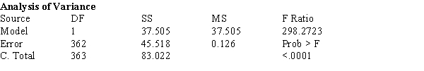
The Des Moines Register recently reported the ratings of high school sportsmanship as compiled by the Iowa High School Athletic Association. For each school the participants and coaches were rated by referees, where 1 = superior, and 5 = unsatisfactory. A regression analysis of the average scores given to football players and coaches is shown below. 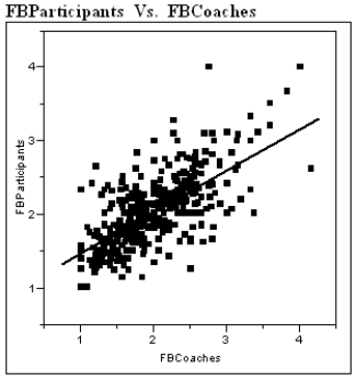 Linear Fit
FBParticipants = 0.902 + 0.568 FBCoaches
a)Interpret the value of the correlation between the ratings of coaches and participants.
b)Interpret the value of the coefficient of determination.
c)Interpret the value of the standard deviation about the least squares line.
Linear FitFBParticipants = 0.902 + 0.568 FBCoaches
a)Interpret the value of the correlation between the ratings of coaches and participants.
b)Interpret the value of the coefficient of determination.
c)Interpret the value of the standard deviation about the least squares line.
Question
The Des Moines Register recently reported the ratings of high school sportsmanship as compiled by the Iowa High School Athletic Association. For each school the spectators and participants were rated by referees, where 1 = superior, and 5 = unsatisfactory. A regression analysis of the average scores given to wrestling spectators and wrestlers is shown below. 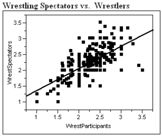 Linear Fit
WrestSpectators = 0.667 + 0.701 Wrestlers
a)Interpret the correlation between the ratings of spectators and wrestlers.
b)Interpret the coefficient of determination.
c)Interpret the value of the standard deviation about the least squares line.
Linear FitWrestSpectators = 0.667 + 0.701 Wrestlers
a)Interpret the correlation between the ratings of spectators and wrestlers.
b)Interpret the coefficient of determination.
c)Interpret the value of the standard deviation about the least squares line.
Question
The data below were gathered on a random sample of 5 basking sharks, swimming through the water and filter-feeding, i.e. passively letting the water bring food into their mouths. 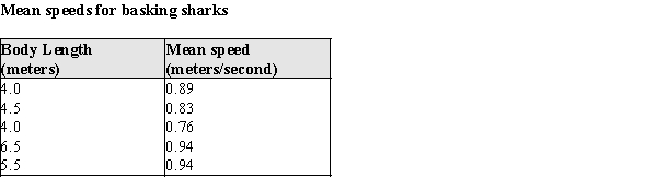
a)What is the value of the correlation coefficient for these data?
b)What is the equation of the least squares line describing the relationship between
x = body length and y = mean speed.
c)If these sharks are representative of the population of basking sharks, what would you predict is the mean speed for a filter-feeding basking shark that is 5.0 meters in length? Show any calculations below.
d)The largest basking shark in the sample is measured as 6.5 meters long. Theory predicts a maximum length of about 12.26 meters. Would it be reasonable to use the equation from part (b) above to predict the mean filter-feeding speed for a 12 meter long basking shark? Why or why not?
Question
Consider the following five scatterplots. All are drawn to the same scale on both the x and y axes. For which scatterplot is the relationship negative?
A)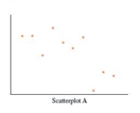
B)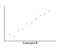
C)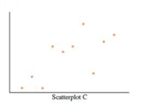
D)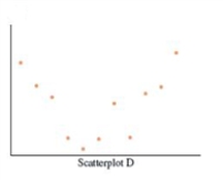
E)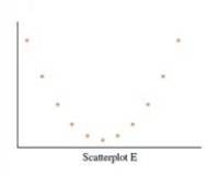
A)
B)
C)
D)
E)
Question
Exhibit 4-1
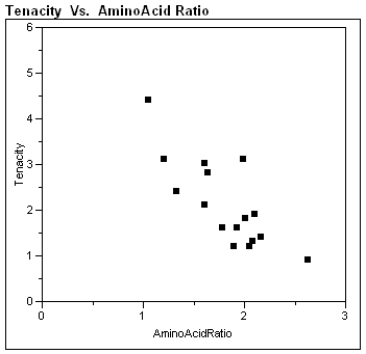
The preservation of objects made of organic material is a constant concern to those caring for items of historical interest. For example, some delicate fabrics are natural silks--they are made of protein and are biodegradable. Many silks in museum collections are in danger of crumbling. It would be of great benefit to be able to assess the delicacy of the fabric before making decisions about displaying it. One possibility is chemical analysis, which might give some evidence about the brittle nature of a fabric. To investigate this possibility, bio-chemical data in the form of a ratio of the amount of certain amino acids in the fibers was acquired from the linings of sixteen 19th and early 20th century Japanese kimonos, and the tenacity (breaking stress) of the fabric was also recorded.
Using the data from the Japanese kimonos, construct the least squares best fit line predicting tenacity using amino acid ratio as a predictor.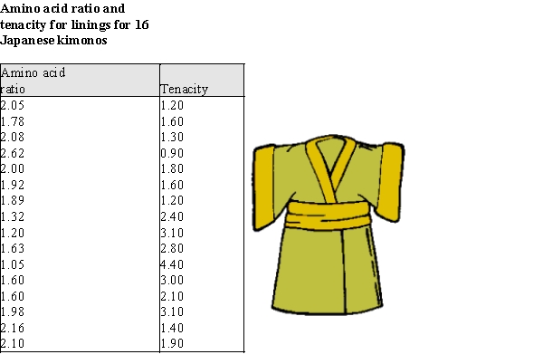
Refer to Exhibit 4-1.
What is the equation of the least-squares line?
Question
Data on x = the weight of a pickup truck (pounds) and y = distance (in feet) required for a truck traveling 40 miles per hour to come to a complete stop for 30 trucks was used to fit the least squares regression line  . Which of the following statements is a correct interpretation of the value 26 in the equation of the regression line?
A)On average, the stopping distance increases by 26 feet for each 1-pound increase in truck weight.
B)On average, the truck weight increases by 26 pounds for each additional foot in stopping distance.
C)On average, the stopping distance is 26 feet when the truck weight is 0.
D)Approximately 26% of the variation in the stopping distances can be explained by the linear relationship between stopping distance and truck weight.
E)It is not reasonable to interpret the intercept in this setting because a weight of 0 is outside the range of the data used to fit the regression line.
. Which of the following statements is a correct interpretation of the value 26 in the equation of the regression line? A)On average, the stopping distance increases by 26 feet for each 1-pound increase in truck weight.
B)On average, the truck weight increases by 26 pounds for each additional foot in stopping distance.
C)On average, the stopping distance is 26 feet when the truck weight is 0.
D)Approximately 26% of the variation in the stopping distances can be explained by the linear relationship between stopping distance and truck weight.
E)It is not reasonable to interpret the intercept in this setting because a weight of 0 is outside the range of the data used to fit the regression line.
Question
The use of small aircraft with human observers is common in wildlife studies where the goal is to estimate the abundance of different species. Recently there has been interest in using unmanned aerial vehicles (UAV). The UAV, something about the size of a model airplane, would fly over the area of interest and take pictures to be analyzed by computers with imagery software when the UAV returns. The plot below is from a test run of the UAV over 10 areas in South Central Florida, using bird decoys to test the reliability of the process. 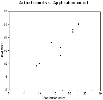 (a)The least squares best fit line is
 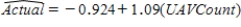 . Plot this line on the graph above. Show any calculations in the space below.
(b)The least squares line is the line that minimizes the sum of the squared residuals. On the graph above pick 2 points and sketch the residuals associated with those points.
(a)The least squares best fit line is . Plot this line on the graph above. Show any calculations in the space below.(b)The least squares line is the line that minimizes the sum of the squared residuals. On the graph above pick 2 points and sketch the residuals associated with those points.
Question
Question
The breeding success of birds that nest on the ground can be affected by the depth of winter snow in high altitudes. The plot below relates the percentage of White-tailed Ptarmigan hens hatching at least one egg, to the amount of snowfall in the Sierra Nevadas that winter. 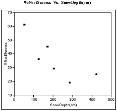 a)The least squares best fit line is %NestSuccess = 55.1816 − 0.092(SnowDepth). Graph this line using the axes above. Show any calculations in the space below.
b)The least squares line is the line that minimizes the sum of the squared residuals. On the graph above pick 2 points and sketch the residuals associated with those points.
a)The least squares best fit line is %NestSuccess = 55.1816 − 0.092(SnowDepth). Graph this line using the axes above. Show any calculations in the space below.b)The least squares line is the line that minimizes the sum of the squared residuals. On the graph above pick 2 points and sketch the residuals associated with those points.
Question
Exhibit 4-3
Paleontology, the study of forms of prehistoric life, can sometimes be aided by modern biology. The study of prehistoric birds depends on fossil information, which typically consists of imprints in stone of a prehistoric creature's remains. To study the productivity of an ancient ecosystem it would be useful know the actual mass of the individual birds, but this information is not preserved in the fossil record. It seems reasonable that the biomechanics of birds operates much the same today as in the past. For example, relationship between the wing length and total weight of a bird should be very similar today to the relationship in the distant past. The wing lengths of ancient birds are readily obtainable from the fossil record, but the weight is not. Assuming similar biomechanical development for ancient birds and modern birds, a regression model expressing the relationship between wing length and total weight of a modern bird could be used to estimate the mass of similar prehistoric birds and thus gauge some aspects of the ancient ecosystem.
Data is available for some modern birds of prey. Specifically, data on the mean wing length and mean total weight of species of hawk-like birds of prey is given below.
Refer to Exhibit 4-3. What is the equation of the least-squares line?
Question
The data below were gathered on a random sample of 7 male black-footed albatrosses of known age. In an effort to monitor diseases of these animals, biologists would like to be able to estimate the age of animals that have died by flattening their gonads and measuring the resulting area. 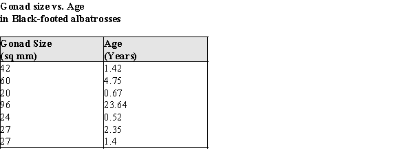
a)What is the value of the correlation coefficient for these data?
b)What is the equation of the least squares line describing the relationship between x = Gonad Size and y = Age.
c)If these albatrosses are representative of the population, what would you predict to be the age of a male albatross with a gonad size of 50 sq. mm? Show any calculations below.
d)The largest albatross gonad size in the sample was 96 sq mm, with an age of 23.64 years. These animals are thought to live for up to 40 years. Would it be reasonable to use the equation from part (b) above to predict the age for a gonad size of 150 sq mm? Why or why not?
Question
If a scatter plot exhibits a strong negative relationship, what can be said about the value of the quantity,  ?
?
? Question
Question
In the 19th Century, venereal diseases were the major preventable diseases striking soldiers far from home. During the American Civil War, the United States Army kept records on soldiers diagnosed with syphilis and gonorrhea. An analysis of the incidence of these diseases is presented below. (Incidence is the rate of increase in the number of cases--for these data, the incidence is number of soldiers per 100,000 per month.) 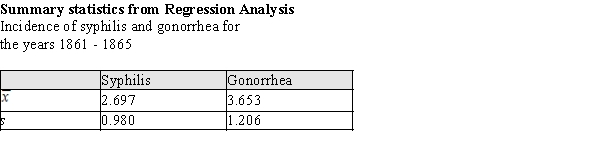
r = 0.914,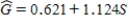 a)If, at a particular point in time, the incidence rate for Syphilis is one standard deviation above the mean, what would be the predicted incidence rate for gonorrhea?
r = 0.914,
a)If, at a particular point in time, the incidence rate for Syphilis is one standard deviation above the mean, what would be the predicted incidence rate for gonorrhea? Question
Twenty-five assembly-line workers participated in a study to investigate the relationship between experience and the amount of time required to complete an assembly task. Assembly time (in minutes) and number of months the worker had been employed on the assembly line were measured for each worker. The resulting data on y = time to complete assembly and x = number of months on the assembly line were used to produce the scatterplot and computer output below. 
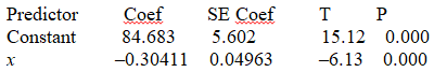
S = 9.79097 R-Sq = 62.0% R-Sq(adj) = 60.4%
Which of the following is the value of the intercept of the least squares regression line?
A)5.602
B)-0.30411
C)0.04963
D)15.12
E)84.683
S = 9.79097 R-Sq = 62.0% R-Sq(adj) = 60.4%
Which of the following is the value of the intercept of the least squares regression line?
A)5.602
B)-0.30411
C)0.04963
D)15.12
E)84.683
Question
When children and adolescents are discharged from the hospital the parents may still provide substantial care, such as the insertion of a feeding tube through the nose and down the esophagus into the stomach. It is difficult for parents to know how far to insert the tube, especially with rapidly growing infants. It may be possible for parents to measure their child's height and from that calculate the appropriate insertion length using a regression equation. At a major children's hospital, children and adolescents' heights and esophageal lengths were measured and a regression analysis performed. The data from this analysis is summarized below: 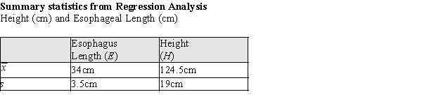 r = 0.995,
  = 11.476 + 0.181H
a)For a child with a height one standard deviation above the mean, what would be the predicted esophageal length?
b)What proportion of the variability in esophageal length is accounted for by the height of the children and adolescents?
c)From the information presented above, does it appear that the esophagus length can be accurately predicted from the height of young patients? Provide statistical evidence for your response.
r = 0.995, = 11.476 + 0.181Ha)For a child with a height one standard deviation above the mean, what would be the predicted esophageal length?
b)What proportion of the variability in esophageal length is accounted for by the height of the children and adolescents?
c)From the information presented above, does it appear that the esophagus length can be accurately predicted from the height of young patients? Provide statistical evidence for your response.
Question
Exhibit 4-3
Paleontology, the study of forms of prehistoric life, can sometimes be aided by modern biology. The study of prehistoric birds depends on fossil information, which typically consists of imprints in stone of a prehistoric creature's remains. To study the productivity of an ancient ecosystem it would be useful know the actual mass of the individual birds, but this information is not preserved in the fossil record. It seems reasonable that the biomechanics of birds operates much the same today as in the past. For example, relationship between the wing length and total weight of a bird should be very similar today to the relationship in the distant past. The wing lengths of ancient birds are readily obtainable from the fossil record, but the weight is not. Assuming similar biomechanical development for ancient birds and modern birds, a regression model expressing the relationship between wing length and total weight of a modern bird could be used to estimate the mass of similar prehistoric birds and thus gauge some aspects of the ancient ecosystem.
Data is available for some modern birds of prey. Specifically, data on the mean wing length and mean total weight of species of hawk-like birds of prey is given below.
Refer to Exhibit 4-3. Approximately what proportion of the variability in weight is explained by the wing length?
Question
Exhibit 4-1
The preservation of objects made of organic material is a constant concern to those caring for items of historical interest. For example, some delicate fabrics are natural silks--they are made of protein and are biodegradable. Many silks in museum collections are in danger of crumbling. It would be of great benefit to be able to assess the delicacy of the fabric before making decisions about displaying it. One possibility is chemical analysis, which might give some evidence about the brittle nature of a fabric. To investigate this possibility, bio-chemical data in the form of a ratio of the amount of certain amino acids in the fibers was acquired from the linings of sixteen 19th and early 20th century Japanese kimonos, and the tenacity (breaking stress) of the fabric was also recorded.
Using the data from the Japanese kimonos, construct the least squares best fit line predicting tenacity using amino acid ratio as a predictor.
Refer to Exhibit 4-1.
Approximately what proportion of the variability in tenacity is explained by the amino acid ratio?
Question
Question
Exhibit 4-2
The theory of fiber strength suggests that the relationship between fiber tenacity and amino acid ratio is logarithmic, i.e.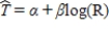 , where T is the tenacity and R is the amino acid ratio.
Perform the appropriate transformation of variable(s) and fit this logarithmic model to the data.
Refer to Exhibit 4-2.
What is the resulting best fit line using this model?
The theory of fiber strength suggests that the relationship between fiber tenacity and amino acid ratio is logarithmic, i.e.
, where T is the tenacity and R is the amino acid ratio.
Perform the appropriate transformation of variable(s) and fit this logarithmic model to the data.
Refer to Exhibit 4-2.
What is the resulting best fit line using this model?
Question
Question
Exhibit 4-4:
Biological theory suggests that the relationship between the weight of these animals and their wing length is exponential, i.e. W = α(10)βL, or W = α(e)βL where W is the wing weight and L is the wing length.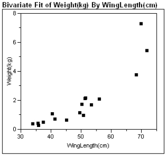
Refer to Exhibit 4-4.
For a wing length of the data point where L = 56.0 (Hieraeus fasciatus), what is the predicted bird weight? Show your work below.
Question
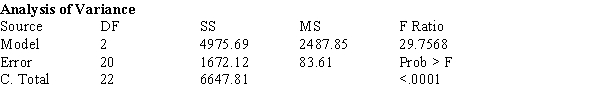
A common statistical method for estimating a population size assumes each member of the population has an equal probability of being captured. To assess this assumption for crocodile populations, investigators repeatedly sampled sections of rivers in Australia. Crocodile lengths were measured in size classes. Crocs 0.0 - 0.3 meters in length are in size class 1, 0.3 - 0.6 meters in length are size class 2, etc. The normal maximum adult length is in a class size of 9 or 10. The investigators fit a quadratic function relating the probability of capture and the size class of captured crocodiles. The output from their analysis is shown below. 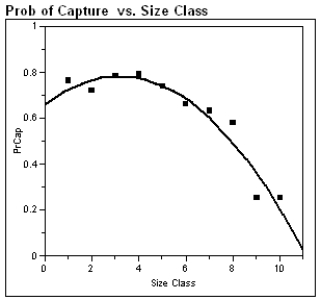 Polynomial Fit Degree=2
PrCap = 0.66 + 0.77Class − 0.01(Class)^2
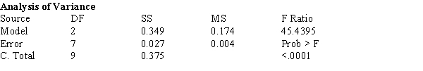
(a)What proportion of the variability in probability of capture is explained by the crocodile's size class?
(b)Some biologists speculate that as crocodiles grow they become more wary of humans, and are more difficult to detect in the wild. Support or refute this belief by appealing to the analysis above.
Polynomial Fit Degree=2PrCap = 0.66 + 0.77Class − 0.01(Class)^2
(a)What proportion of the variability in probability of capture is explained by the crocodile's size class?
(b)Some biologists speculate that as crocodiles grow they become more wary of humans, and are more difficult to detect in the wild. Support or refute this belief by appealing to the analysis above.
Question
Exhibit 4-2
The theory of fiber strength suggests that the relationship between fiber tenacity and amino acid ratio is logarithmic, i.e. , where T is the tenacity and R is the amino acid ratio.
Perform the appropriate transformation of variable(s) and fit this logarithmic model to the data.
Refer to Exhibit 4-2. Does it appear that the transformed model is no improvement over the linear model, a slight improvement, or a significant improvement? Justify your response with an appropriate statistical argument.
The theory of fiber strength suggests that the relationship between fiber tenacity and amino acid ratio is logarithmic, i.e.
, where T is the tenacity and R is the amino acid ratio.
Perform the appropriate transformation of variable(s) and fit this logarithmic model to the data.
Refer to Exhibit 4-2. Does it appear that the transformed model is no improvement over the linear model, a slight improvement, or a significant improvement? Justify your response with an appropriate statistical argument.
Question
Question
Question
Polar bear cubs are born in the winter in dens, and they must live off the fat stores of the mother even after leaving the den for sea ice, since the availability of their prey is unpredictable. Therefore, maternal weight is an important factor in successful reproduction of polar bears. In a recent spring, 261 adult females with 492 cubs were captured as they left their dens, and the mothers' weight and ages were determined by "counting annuli in the cementum of an extracted vestigial premolar tooth." (We are NOT making this up!) A quadratic fit of the maternal weight in kilograms to age in years resulted in the regression analysis below. 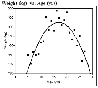 Polynomial Fit Degree=2
Weight = 82.920 + 12.134 Age − 0.360(Age )^2
a)On average, about how far off are the weights of the maternal bears? That is, what is a typical difference between the actual weights and the weights predicted by the quadratic model?
b)If the maternal weight is an important factor as discussed above, what age of the female would seem to be the best for reproduction success? In a few sentences, justify your answer by appealing to the information provided above.
Polynomial Fit Degree=2Weight = 82.920 + 12.134 Age − 0.360(Age )^2
a)On average, about how far off are the weights of the maternal bears? That is, what is a typical difference between the actual weights and the weights predicted by the quadratic model?
b)If the maternal weight is an important factor as discussed above, what age of the female would seem to be the best for reproduction success? In a few sentences, justify your answer by appealing to the information provided above.
Question
Exhibit 4-2
The theory of fiber strength suggests that the relationship between fiber tenacity and amino acid ratio is logarithmic, i.e. , where T is the tenacity and R is the amino acid ratio.
Perform the appropriate transformation of variable(s) and fit this logarithmic model to the data.
Refer to Exhibit 4-2.
For an amino acid ratio of R = 1.5, what is the predicted tenacity?
The theory of fiber strength suggests that the relationship between fiber tenacity and amino acid ratio is logarithmic, i.e.
, where T is the tenacity and R is the amino acid ratio.
Perform the appropriate transformation of variable(s) and fit this logarithmic model to the data.
Refer to Exhibit 4-2.
For an amino acid ratio of R = 1.5, what is the predicted tenacity?
Question
Exhibit 4-6
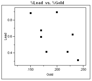
During the first 3 centuries AD, the Roman Empire produced coins in the Eastern provinces. Some historians argue that not all these coins were produced in Roman mints, and further that local provincial mints struck some of them. Because the "style" of coins is difficult to analyze, the historians would like to use metallurgical analysis as one tool to identify the source mints of these coins. Investigators studied 8 coins known to have been produced by the mint in Rome in an attempt to identify a trace element profile for these coins, and have identified gold and lead as possible factors in identifying other coins as having been minted in Rome. The gold and lead content, measured as a % of weight of each coin, is given in the table, and a scatter plot of these data is presented below.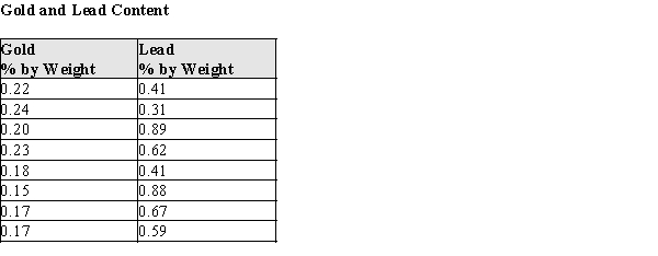
Refer to Exhibit 4-6.
a)What is the equation of the least squares best fit line?
b)Sketch the best fit line on the scatter plot.
c)What is the value of the correlation coefficient? Interpret this value.
d)What is the value of the coefficient of determination? Give an interpretation of this value.
Question
Question
Exhibit 4-7
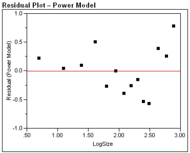
Golden-rumped elephant shrews have long flexible snouts, used to overturn leaf-litter where they find their food: millipedes, insects and spiders. These animals are among the approximately 10% of mammalian species that mate for life. Just why these mammals are monogamous is poorly understood, and one theory is that a monogamous male would have to defend less territory from intrusion by other males. The home range of an animal, i.e. that area over which they typically travel, is a function of diet and energy consumption of the animal. The energy consumption is, in turn, typically a function of the animal's size. In a recent study, investigators reasoned that if monogamy was related in some way to the home territory, this should be detectable by comparing these animals to other insect-eating mammals. Data were gathered on 27 similar species and are presented in the table below.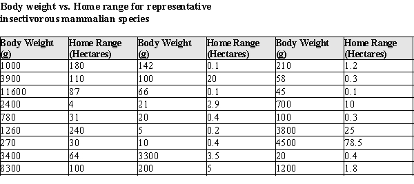 After fitting a straight line model,
  , significant curvature was detected in the residual plot, and two transformed models were chosen for further analysis: the power and exponential models. The computer output for these transformed models and the residual plots follow.
Residual Plot and Statistical Analysis - exponential model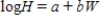
 Log Home Range vs. Weight
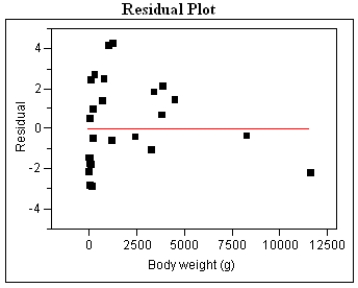
Log(H) = 0.250 + 0.000231 W Residual Plot and Statistical Analysis - Power model
 Log Home Range vs. Log Weight
Log(H) = −1.601 + 0.893Log(W)
Refer to Exhibit 4-7. These shrews typically weigh 550g and their home range is about 2.9 hectares. Using your preferred model from part (c), locate the Golden-rumped elephant shrew on the appropriate residual plot by marking with a small "x." Does your placement of this point suggest the monogamy of these shrews sets them apart from similar species? In a few sentences, explain why or why not.
Golden-rumped elephant shrews have long flexible snouts, used to overturn leaf-litter where they find their food: millipedes, insects and spiders. These animals are among the approximately 10% of mammalian species that mate for life. Just why these mammals are monogamous is poorly understood, and one theory is that a monogamous male would have to defend less territory from intrusion by other males. The home range of an animal, i.e. that area over which they typically travel, is a function of diet and energy consumption of the animal. The energy consumption is, in turn, typically a function of the animal's size. In a recent study, investigators reasoned that if monogamy was related in some way to the home territory, this should be detectable by comparing these animals to other insect-eating mammals. Data were gathered on 27 similar species and are presented in the table below.
After fitting a straight line model, , significant curvature was detected in the residual plot, and two transformed models were chosen for further analysis: the power and exponential models. The computer output for these transformed models and the residual plots follow.Residual Plot and Statistical Analysis - exponential model
Log Home Range vs. WeightLog(H) = 0.250 + 0.000231 W
Residual Plot and Statistical Analysis - Power model Log Home Range vs. Log WeightLog(H) = −1.601 + 0.893Log(W)
Refer to Exhibit 4-7. These shrews typically weigh 550g and their home range is about 2.9 hectares. Using your preferred model from part (c), locate the Golden-rumped elephant shrew on the appropriate residual plot by marking with a small "x." Does your placement of this point suggest the monogamy of these shrews sets them apart from similar species? In a few sentences, explain why or why not.
Question
One of the problems when estimating the size of animal populations from aerial surveys is that animals may bunch together, making it difficult to distinguish and count them accurately. For example, a horse standing alone is easy to spot; if seven horses huddled close together some may be missed, resulting in an undercount. The relative frequency of undercounts is typically reported as a percent. For example, if there are 10 horses in a group, a person in the plane may typically count fewer than 10 horses 20% of the time. In a recent study, the percent of sightings that resulted in an undercount was related to the size of the "group" of horses and donkeys; the following data were gathered: 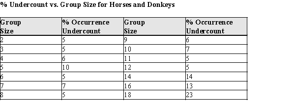 After fitting a straight line model,
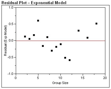
  , significant curvature was detected in the residual plot, and two nonlinear models were chosen for further analysis, the exponential and the power models. The computer output for these models is given below, and the residual plots follow.
 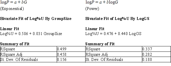 Residual Plots
 a)For the exponential model, calculate the predicted log (%undercount) for a group size = 10.
b)Use your calculations from part (a) to predict the %undercount for a group size = 10.
c)Generally speaking, which of the two models, power or exponential, is better at predicting the log (Percent Undercount)? Provide statistical justification for your choice.
After fitting a straight line model, , significant curvature was detected in the residual plot, and two nonlinear models were chosen for further analysis, the exponential and the power models. The computer output for these models is given below, and the residual plots follow. Residual Plots a)For the exponential model, calculate the predicted log (%undercount) for a group size = 10.b)Use your calculations from part (a) to predict the %undercount for a group size = 10.
c)Generally speaking, which of the two models, power or exponential, is better at predicting the log (Percent Undercount)? Provide statistical justification for your choice.
Question
Exhibit 4-7
Golden-rumped elephant shrews have long flexible snouts, used to overturn leaf-litter where they find their food: millipedes, insects and spiders. These animals are among the approximately 10% of mammalian species that mate for life. Just why these mammals are monogamous is poorly understood, and one theory is that a monogamous male would have to defend less territory from intrusion by other males. The home range of an animal, i.e. that area over which they typically travel, is a function of diet and energy consumption of the animal. The energy consumption is, in turn, typically a function of the animal's size. In a recent study, investigators reasoned that if monogamy was related in some way to the home territory, this should be detectable by comparing these animals to other insect-eating mammals. Data were gathered on 27 similar species and are presented in the table below. After fitting a straight line model, , significant curvature was detected in the residual plot, and two transformed models were chosen for further analysis: the power and exponential models. The computer output for these transformed models and the residual plots follow.
Residual Plot and Statistical Analysis - exponential model Log Home Range vs. Weight
Log(H) = 0.250 + 0.000231 W Residual Plot and Statistical Analysis - Power model Log Home Range vs. Log Weight
Log(H) = −1.601 + 0.893Log(W)
Refer to Exhibit 4-7.
For the exponential model, calculate the predicted log (Home Range) for a Weight of 1000g.
Golden-rumped elephant shrews have long flexible snouts, used to overturn leaf-litter where they find their food: millipedes, insects and spiders. These animals are among the approximately 10% of mammalian species that mate for life. Just why these mammals are monogamous is poorly understood, and one theory is that a monogamous male would have to defend less territory from intrusion by other males. The home range of an animal, i.e. that area over which they typically travel, is a function of diet and energy consumption of the animal. The energy consumption is, in turn, typically a function of the animal's size. In a recent study, investigators reasoned that if monogamy was related in some way to the home territory, this should be detectable by comparing these animals to other insect-eating mammals. Data were gathered on 27 similar species and are presented in the table below.
After fitting a straight line model, , significant curvature was detected in the residual plot, and two transformed models were chosen for further analysis: the power and exponential models. The computer output for these transformed models and the residual plots follow.Residual Plot and Statistical Analysis - exponential model
Log Home Range vs. WeightLog(H) = 0.250 + 0.000231 W
Residual Plot and Statistical Analysis - Power model Log Home Range vs. Log WeightLog(H) = −1.601 + 0.893Log(W)
Refer to Exhibit 4-7.
For the exponential model, calculate the predicted log (Home Range) for a Weight of 1000g.
Question
Exhibit 4-5
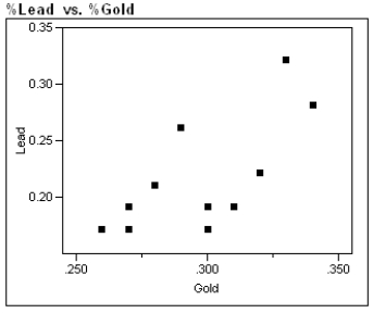
During the first 3 centuries AD, the Roman Empire produced coins in the Eastern provinces. Some historians argue that not all these coins were produced in local mints, and further that the mint of Rome struck some of them. Because the "style" of coins is difficult to analyze, the historians would like to use metallurgical analysis as one tool to identify the source mints of these coins. Investigators studied 11 coins known to have been produced by local mints in an attempt to identify a trace element profile for these coins, and have identified gold and lead as possible factors in identifying other coins as having been locally minted. The gold and lead content, measured as a % of weight of each coin, is given in the table, and a scatter plot of these data is presented below.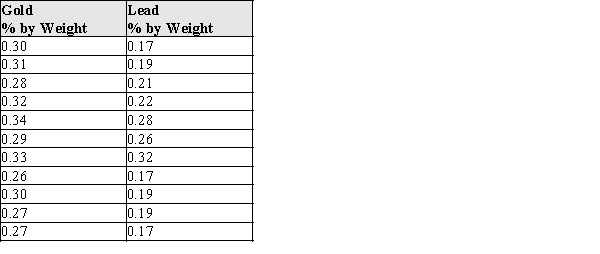
Refer to Exhibit 4-5.
a)What is the equation of the least squares best fit line?
b)Sketch the best fit line on the scatter plot.
c)What is the value of the correlation coefficient? Interpret this value.
d)What is the value of the coefficient of determination? Give an interpretation of this value.
Question
Exhibit 4-4:
Biological theory suggests that the relationship between the weight of these animals and their wing length is exponential, i.e. W = α(10)βL, or W = α(e)βL where W is the wing weight and L is the wing length.
Refer to Exhibit 4-4. What is the resulting best fit line using the transformed model?
Biological theory suggests that the relationship between the weight of these animals and their wing length is exponential, i.e. W = α(10)βL, or W = α(e)βL where W is the wing weight and L is the wing length.
Refer to Exhibit 4-4. What is the resulting best fit line using the transformed model?
Question
To confirm Ohm's law, the student measures the voltage versus current for the conductor sample. The student changes the current through the conductor from 0 to 2 mA every 20 seconds increasing the current by 0.2 mA and measures the corresponding voltage value. The results of these measurements are presented in the table below. 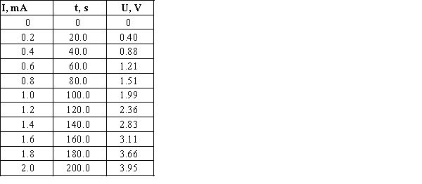 Find the correlation coefficients for the obtained data and make your conclusions about thestatistical relationships between current and voltage and between time and voltage. Can we conclude that correlations imply causation for these pairs of variables?
A)Both correlation coefficients are very close to 1, so the relationships are very strong.Both of these relationships imply causation.
B)Both correlation coefficients are very close to 1, so the relationships are very strong.The change of current causes the change of voltage, but the change of time without changing current does not cause the change of voltage.
C)Both correlation coefficients are very close to 1, so the relationships are weak.The change of current can cause the change of voltage, but the change of time without changing current does not cause the change of voltage.
D)Both correlation coefficients are very close to 1, so the relationships are weak.Both current and time do not imply on the voltage of the conductor sample.
Find the correlation coefficients for the obtained data and make your conclusions about thestatistical relationships between current and voltage and between time and voltage. Can we conclude that correlations imply causation for these pairs of variables?A)Both correlation coefficients are very close to 1, so the relationships are very strong.Both of these relationships imply causation.
B)Both correlation coefficients are very close to 1, so the relationships are very strong.The change of current causes the change of voltage, but the change of time without changing current does not cause the change of voltage.
C)Both correlation coefficients are very close to 1, so the relationships are weak.The change of current can cause the change of voltage, but the change of time without changing current does not cause the change of voltage.
D)Both correlation coefficients are very close to 1, so the relationships are weak.Both current and time do not imply on the voltage of the conductor sample.
Question
As early as 3 years of age, children begin to show preferences for playing with members of their own sex, and report having more same-sex than opposite-sex friends. In a study of 3rd and 4th graders' views on 48 personality traits, children were asked to rate on a "5-point" scale:
−2
= "someone possessing that trait is probably a boy"
−1
= "someone possessing that trait might be a boy"
0
= "can't tell"
1
= "someone possessing that trait might be a girl"
2
= "someone possessing that trait is probably a girl"
A plot of the data is presented below. A single point represents the (average girls' rating, average boys' rating) for a given trait.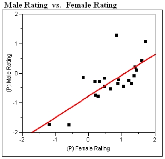 Linear Fit
MRating = −0.765 + 0.714 FRating
a)Circle the single point which represents the most influential observation. What aspect of this point makes it the most influential?
b)Suppose a personality trait similar to those used in the survey were given a 0.0 rating ("can't tell") by the girls. The predicted boys' average rating would be closest to which of the 5 categories described above?
c)The traits plotted above are those the researchers believe are "positive" traits, such as "mature," "honest," and "polite." The researchers thought that girls would rate these positive traits as characteristic of girls to a greater extent than boys would. What aspects of the plot and/or regression analysis presented above are consistent with this thinking?
−2
= "someone possessing that trait is probably a boy"
−1
= "someone possessing that trait might be a boy"
0
= "can't tell"
1
= "someone possessing that trait might be a girl"
2
= "someone possessing that trait is probably a girl"
A plot of the data is presented below. A single point represents the (average girls' rating, average boys' rating) for a given trait.
Linear FitMRating = −0.765 + 0.714 FRating
a)Circle the single point which represents the most influential observation. What aspect of this point makes it the most influential?
b)Suppose a personality trait similar to those used in the survey were given a 0.0 rating ("can't tell") by the girls. The predicted boys' average rating would be closest to which of the 5 categories described above?
c)The traits plotted above are those the researchers believe are "positive" traits, such as "mature," "honest," and "polite." The researchers thought that girls would rate these positive traits as characteristic of girls to a greater extent than boys would. What aspects of the plot and/or regression analysis presented above are consistent with this thinking?
Question
Exhibit 4-7
Golden-rumped elephant shrews have long flexible snouts, used to overturn leaf-litter where they find their food: millipedes, insects and spiders. These animals are among the approximately 10% of mammalian species that mate for life. Just why these mammals are monogamous is poorly understood, and one theory is that a monogamous male would have to defend less territory from intrusion by other males. The home range of an animal, i.e. that area over which they typically travel, is a function of diet and energy consumption of the animal. The energy consumption is, in turn, typically a function of the animal's size. In a recent study, investigators reasoned that if monogamy was related in some way to the home territory, this should be detectable by comparing these animals to other insect-eating mammals. Data were gathered on 27 similar species and are presented in the table below. After fitting a straight line model, , significant curvature was detected in the residual plot, and two transformed models were chosen for further analysis: the power and exponential models. The computer output for these transformed models and the residual plots follow.
Residual Plot and Statistical Analysis - exponential model Log Home Range vs. Weight
Log(H) = 0.250 + 0.000231 W Residual Plot and Statistical Analysis - Power model Log Home Range vs. Log Weight
Log(H) = −1.601 + 0.893Log(W)
Refer to Exhibit 4-7.
Generally speaking, which of the two models, power or exponential, is better at predicting the log (Home Range)? Provide statistical justification for your choice.
Golden-rumped elephant shrews have long flexible snouts, used to overturn leaf-litter where they find their food: millipedes, insects and spiders. These animals are among the approximately 10% of mammalian species that mate for life. Just why these mammals are monogamous is poorly understood, and one theory is that a monogamous male would have to defend less territory from intrusion by other males. The home range of an animal, i.e. that area over which they typically travel, is a function of diet and energy consumption of the animal. The energy consumption is, in turn, typically a function of the animal's size. In a recent study, investigators reasoned that if monogamy was related in some way to the home territory, this should be detectable by comparing these animals to other insect-eating mammals. Data were gathered on 27 similar species and are presented in the table below.
After fitting a straight line model, , significant curvature was detected in the residual plot, and two transformed models were chosen for further analysis: the power and exponential models. The computer output for these transformed models and the residual plots follow.Residual Plot and Statistical Analysis - exponential model
Log Home Range vs. WeightLog(H) = 0.250 + 0.000231 W
Residual Plot and Statistical Analysis - Power model Log Home Range vs. Log WeightLog(H) = −1.601 + 0.893Log(W)
Refer to Exhibit 4-7.
Generally speaking, which of the two models, power or exponential, is better at predicting the log (Home Range)? Provide statistical justification for your choice.
Question
For the given scatterplot, identify if there is a relationship between  and
and  . If there is a relationship between the variables, define, if it is linear or nonlinear. If the relationship appears to be linear, determine the direction and the strength of this relationship.
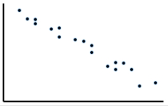
A)Based on the value of the correlation coefficient , we can conclude that there is a weak negative nonlinear relationship.
B)Based on the value of the correlation coefficient , we can conclude that there is a strong positive nonlinear relationship.
C)Based on the value of the correlation coefficient , we can conclude that there is a weak positive linear relationship.
D)Based on the value of the correlation coefficient , we can conclude that there is a strong negative linear relationship.
and . If there is a relationship between the variables, define, if it is linear or nonlinear. If the relationship appears to be linear, determine the direction and the strength of this relationship. A)Based on the value of the correlation coefficient
, we can conclude that there is a weak negative nonlinear relationship.B)Based on the value of the correlation coefficient
, we can conclude that there is a strong positive nonlinear relationship.C)Based on the value of the correlation coefficient
, we can conclude that there is a weak positive linear relationship.D)Based on the value of the correlation coefficient
, we can conclude that there is a strong negative linear relationship. Question
Identify linear patterns in the scatterplots shown.
A)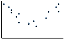
B)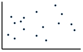
C)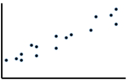
D)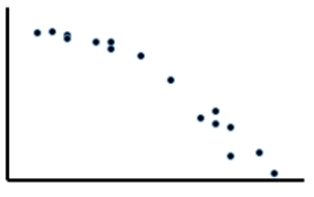
A)
B)
C)
D)
Question
According to the information of the Council of graduate schools ( "http://cgsnet.org/cgs-international-graduate-admissions-survey-reports" , the total number of non-U.S. graduates applying for admission to the master's and doctoral degree programs in U.S. colleges and universities has been increasing year-to-year from 2010. 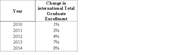
A)Predictor is a year, and response variable is a total graduate enrollment.
B)Predictor is a total graduate enrollment, and response variable is a year.
A)Predictor is a year, and response variable is a total graduate enrollment.
B)Predictor is a total graduate enrollment, and response variable is a year.
Question
For the given scatterplot, identify if there is a relationship between  and
and  . If there is a relationship between the variables, define, if it is linear or nonlinear. If the relationship appears to be linear, determine the direction and the strength of this relationship.
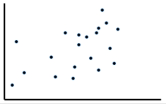
A)Based on the value of the correlation coefficient , we can conclude that there is a weak positive linear relationship.
B)Based on the value of the correlation coefficient , we can conclude that there is a strong positive nonlinear relationship.
C)Based on the value of the correlation coefficient , we can conclude that there is a weak positive linear relationship.
D)Based on the value of the correlation coefficient , we can conclude that there is a strong positive nonlinear relationship.
and . If there is a relationship between the variables, define, if it is linear or nonlinear. If the relationship appears to be linear, determine the direction and the strength of this relationship. A)Based on the value of the correlation coefficient
, we can conclude that there is a weak positive linear relationship.B)Based on the value of the correlation coefficient
, we can conclude that there is a strong positive nonlinear relationship.C)Based on the value of the correlation coefficient
, we can conclude that there is a weak positive linear relationship.D)Based on the value of the correlation coefficient
, we can conclude that there is a strong positive nonlinear relationship. Question
The plot given below shows the points and the regression lines for the data set on the same graph. The blue line is the regression line for all points. The red line is the regression line for the data points excluding those which influence observation. 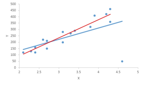 Describe the effect of the influential observation on the equation of the least squares regression line. Select the correct statement.
A)The influential observation changes the equation of the regression line.
B)The influential observation is located long far from the other data points.
C)The influential observation only increases the error of estimation.
D)The influential observation is always an outlier.
Describe the effect of the influential observation on the equation of the least squares regression line. Select the correct statement.A)The influential observation changes the equation of the regression line.
B)The influential observation is located long far from the other data points.
C)The influential observation only increases the error of estimation.
D)The influential observation is always an outlier.
Question
In the season 2016-2017 Chelsea won English Premier League. Ron and Tom, fans of Chelsea, argued which factor was more important for winning the League: the number of goals scored or the number of goals conceded. Using the information about the results of the season 2016-2017 represented in the table below ( http://www.espn.com/soccer/standings/_/league/eng.1/season/2016/sort/points), find out, which factor has been statistically more important. 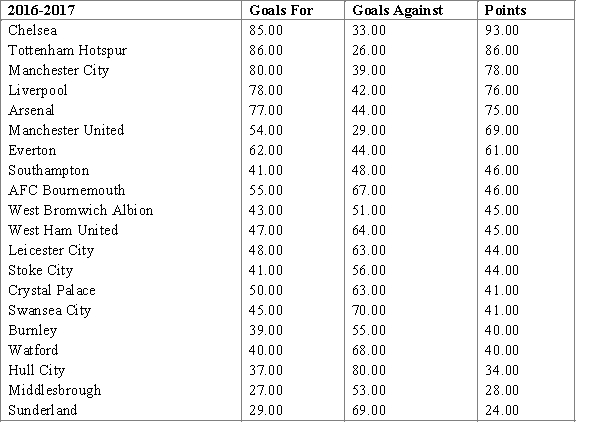
A)The correlation coefficient between the goals scored (goals for) and the points is close to 1, so there is a strong positive linear relationship.The correlation coefficient between the goals conceded (goals against) and the points
  is negative, so there is a weak linear relationship.So statistically more important factor is the number of goals scored.
B)The absolute value of the correlation coefficient between the goals scored (goals for) and the points is greater than the absolute value of the correlation coefficient between the goals conceded (goals against) and the points
  , so statistically more important factor is the number of goals scored.
C)The correlation coefficient between the goals scored (goals for) and the points is close to 1, so there is a strong positive linear relationship.The correlation coefficient between the goals conceded (goals against) and the points
  is negative, so there is a weak linear relationship.So statistically more important factor is the number of goals scored.
D)The absolute value of the correlation coefficient between the goals scored (goals for) and the points is less than the absolute value of the correlation coefficient between the goals conceded (goals against) and the points
  , so statistically more important factor is the number of goals conceded.
A)The correlation coefficient between the goals scored (goals for) and the points
is close to 1, so there is a strong positive linear relationship.The correlation coefficient between the goals conceded (goals against) and the points is negative, so there is a weak linear relationship.So statistically more important factor is the number of goals scored.B)The absolute value of the correlation coefficient between the goals scored (goals for) and the points
is greater than the absolute value of the correlation coefficient between the goals conceded (goals against) and the points , so statistically more important factor is the number of goals scored.C)The correlation coefficient between the goals scored (goals for) and the points
is close to 1, so there is a strong positive linear relationship.The correlation coefficient between the goals conceded (goals against) and the points is negative, so there is a weak linear relationship.So statistically more important factor is the number of goals scored.D)The absolute value of the correlation coefficient between the goals scored (goals for) and the points
is less than the absolute value of the correlation coefficient between the goals conceded (goals against) and the points , so statistically more important factor is the number of goals conceded. Question
We know that the linear regression must be used if we have a strong relationship between  and
and  (or in other words when
  is proportional to
  ). Choose the statement that best describes the values of
  and
and  which indicate the fact that the relationship is very strong.
A)The value of is very large and the value of
  is close to 1.
B)The value of is very large and the value of
  is close to 0.
C)The value of is small and the value of
  is close to 0.
D)The value of is small and the value of
  is close to 1.
and (or in other words when is proportional to ). Choose the statement that best describes the values of and which indicate the fact that the relationship is very strong. A)The value of
is very large and the value of is close to 1.B)The value of
is very large and the value of is close to 0.C)The value of
is small and the value of is close to 0.D)The value of
is small and the value of is close to 1. Question
According to the Hooke's Law the force (  ) needed to extend or compress a spring by some distance scales linearly with respect to that distance. Student measures the force exerted on the spring versus spring extension. The results of student's measurements are presented in the table below.
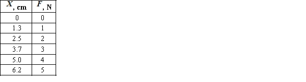
Student observed that the values have the correlation coefficient close to 1, and filled in the table for the values , 7,and 8 newtons. However, the professor noticed the deception, drawing attention to the fact that the student could not get such value of extension for the force of 8 newtons. Calculate the predicted value for 8 N and explain why this value can be incorrect.
A)Predicted value for is 9.9 centimeters.The least squares regression line should not be used to make predictions outside the range of the values because there is no evidence that the linear pattern continues outside this range.
B)Predicted value for is 12.4 centimeters.The least squares regression line should not be used to make predictions outside the range of the values because there is no evidence that the linear pattern continues outside this range.
C)Predicted value for is 9.9 centimeters.The least squares regression line should not be used to make predictions outside the range of the values because a point outside the range will greatly influence the regression line and the resulting parameters will change.
D)Predicted value for is 12.4 centimeters.The least squares regression line should not be used to make predictions outside the range of the values because a point outside the range will greatly influence the regression line and the resulting parameters will change.
) needed to extend or compress a spring by some distance scales linearly with respect to that distance. Student measures the force exerted on the spring versus spring extension. The results of student's measurements are presented in the table below. Student observed that the values have the correlation coefficient close to 1, and filled in the table for the values
, 7,and 8 newtons. However, the professor noticed the deception, drawing attention to the fact that the student could not get such value of extension for the force of 8 newtons. Calculate the predicted value for 8 N and explain why this value can be incorrect.
A)Predicted value for
is 9.9 centimeters.The least squares regression line should not be used to make predictions outside the range of the values because there is no evidence that the linear pattern continues outside this range.B)Predicted value for
is 12.4 centimeters.The least squares regression line should not be used to make predictions outside the range of the values because there is no evidence that the linear pattern continues outside this range.C)Predicted value for
is 9.9 centimeters.The least squares regression line should not be used to make predictions outside the range of the values because a point outside the range will greatly influence the regression line and the resulting parameters will change.D)Predicted value for
is 12.4 centimeters.The least squares regression line should not be used to make predictions outside the range of the values because a point outside the range will greatly influence the regression line and the resulting parameters will change. Question
One should get nice enough grades in the high school to enter the University of Alabama. A survey has been conducted among high school graduates who want to be admitted to the University of Alabama revealing their GPA and SAT scores. The results of this survey are presented in the table below. 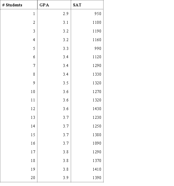 Using this information calculate and interpret the value of the correlation coefficient between GPA and SAT scores of the students.
A)The value of the correlation coefficient , there is a weak positive linear relationship.
B)The value of the correlation coefficient , there is a weak positive nonlinear relationship.
C)The value of the correlation coefficient , there is a strong positive linear relationship.
D)The value of the correlation coefficient , there is a strong positive linear relationship.
Using this information calculate and interpret the value of the correlation coefficient between GPA and SAT scores of the students.A)The value of the correlation coefficient
, there is a weak positive linear relationship.B)The value of the correlation coefficient
, there is a weak positive nonlinear relationship.C)The value of the correlation coefficient
, there is a strong positive linear relationship.D)The value of the correlation coefficient
, there is a strong positive linear relationship. Question
According to official data of "http://www.census.org/" population of Detroit, MI, is decreasing. Use the data from the table below for the population of Detroit to answer the following questions. 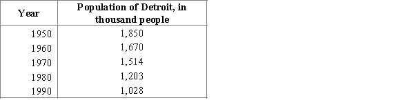 Find the predicted value for the population of Detroit in the year 2000 using the regression line. If the known population of Detroit in the year 2000 is about 951 thousand of people, what can you say about your predicted value? Why is it risky to use the least squares line to make the prediction for the next year?
A)Predicted value is 820 thousand of people.It is noticeably greater than the real value for this year.The least squares regression line should not be used to make predictions outside the range of the x values because there is no evidence that the linear pattern continues outside this range.
B)Predicted value is 853 thousand of people.It is noticeably greater than the real value for this year.The least squares regression line should not be used to make predictions outside the range of the x values because a point outside the range will greatly influence the regression line and the resulting parameters will change.
C)Predicted value is 853 thousand of people.It is noticeably greater than the real value for this year.The least squares regression line should not be used to make predictions outside the range of the x values because there is no evidence that the linear pattern continues outside this range.
D)Predicted value is 820 thousand of people.It is noticeably greater than the real value for this year.The least squares regression line should not be used to make predictions outside the range of the x values because a point outside the range will greatly influence the regression line and the resulting parameters will change.
Find the predicted value for the population of Detroit in the year 2000 using the regression line. If the known population of Detroit in the year 2000 is about 951 thousand of people, what can you say about your predicted value? Why is it risky to use the least squares line to make the prediction for the next year?A)Predicted value is 820 thousand of people.It is noticeably greater than the real value for this year.The least squares regression line should not be used to make predictions outside the range of the x values because there is no evidence that the linear pattern continues outside this range.
B)Predicted value is 853 thousand of people.It is noticeably greater than the real value for this year.The least squares regression line should not be used to make predictions outside the range of the x values because a point outside the range will greatly influence the regression line and the resulting parameters will change.
C)Predicted value is 853 thousand of people.It is noticeably greater than the real value for this year.The least squares regression line should not be used to make predictions outside the range of the x values because there is no evidence that the linear pattern continues outside this range.
D)Predicted value is 820 thousand of people.It is noticeably greater than the real value for this year.The least squares regression line should not be used to make predictions outside the range of the x values because a point outside the range will greatly influence the regression line and the resulting parameters will change.

Unlock Deck
Sign up to unlock the cards in this deck!
Unlock Deck
Unlock Deck
1/70
Play
Full screen (f)
Deck 4: Describing Bivariate Numerical Data
1
If , the standard deviation of y is equal to the standard deviation of the residuals.
, the standard deviation of y is equal to the standard deviation of the residuals.False
2
The least squares line passes through the point .
.True
3
The coefficient of determination is equal to the positive square root of Pearson's r.
False
4
Data were collected on y = price of car (in dollars) and x = age of car (in years) for each car in a sample of 60 used Toyota Camrys. A scatterplot showed a negative linear relationship between x and y. The least squares regression line was fit and the value was computed. If , which of the following is a correct statement?
A)The correlation coefficient is positive, r = 0.55
B)If the least-squares line is used to predict car price based on number of miles driven, predictions should be within $0.55 of the true price.
C)There is a very strong linear relationship between car price and number of miles driven.
D)For each additional mile driven, car price increases by approximately $0.55
E)Approximately 55% of the variability in car price can be explained by the linear relationship between car price and number of miles the car has been driven.
value was computed. If , which of the following is a correct statement? A)The correlation coefficient is positive, r = 0.55
B)If the least-squares line is used to predict car price based on number of miles driven, predictions should be within $0.55 of the true price.
C)There is a very strong linear relationship between car price and number of miles driven.
D)For each additional mile driven, car price increases by approximately $0.55
E)Approximately 55% of the variability in car price can be explained by the linear relationship between car price and number of miles the car has been driven.
Unlock Deck
Unlock for access to all 70 flashcards in this deck.
Unlock Deck
k this deck
5
Twenty-five assembly-line workers participated in a study to investigate the relationship between experience and the amount of time required to complete an assembly task. Assembly time (in minutes) and number of months the worker had been employed on the assembly line were measured for each worker. The resulting data on y= time to complete assembly and x= number of months on the assembly line were used to produce the scatterplot and computer output below.
S= 9.79097 R-Sq = 62.0% R-Sq(adj) = 60.4%
Predict the time required to complete the assembly for an employee with 10 months of experience.
A) 81.6min
B) 90.6min
C) 110.4min
D) 120.7min
E) 150.3min
S= 9.79097 R-Sq = 62.0% R-Sq(adj) = 60.4%
Predict the time required to complete the assembly for an employee with 10 months of experience.
A) 81.6min
B) 90.6min
C) 110.4min
D) 120.7min
E) 150.3min
Unlock Deck
Unlock for access to all 70 flashcards in this deck.
Unlock Deck
k this deck
6
The higher the value of the coefficient of determination, the greater the evidence for a causal relationship between x and y.
Unlock Deck
Unlock for access to all 70 flashcards in this deck.
Unlock Deck
k this deck
7
The value of Pearson's r is always between 0 and 1.
Unlock Deck
Unlock for access to all 70 flashcards in this deck.
Unlock Deck
k this deck
8
Of the following, which is true of Pearson's correlation coefficient, r?
A)The value of r does not depend on the units of y and x.
B)r = 0 indicates a perfect correlation between x and y.
C)r cannot be less than 0 or greater than 1.
D)The value of r depends on which of two variables is labeled x.
E) is greater than 1.0 unless the points on a scatterplot line up exactly.
A)The value of r does not depend on the units of y and x.
B)r = 0 indicates a perfect correlation between x and y.
C)r cannot be less than 0 or greater than 1.
D)The value of r depends on which of two variables is labeled x.
E)
is greater than 1.0 unless the points on a scatterplot line up exactly. Unlock Deck
Unlock for access to all 70 flashcards in this deck.
Unlock Deck
k this deck
9
Which of the following indicates the range of possible values of the coefficient of determination, ?
A)
B)
C)
D)
E)
? A)
B)
C)
D)
E)
Unlock Deck
Unlock for access to all 70 flashcards in this deck.
Unlock Deck
k this deck
10
If r is close to 1, then the points lie close to a straight line with a positive slope.
Unlock Deck
Unlock for access to all 70 flashcards in this deck.
Unlock Deck
k this deck
11
Data on x = the weight of a pickup truck (pounds) and y = distance (in feet) required for a truck traveling 40 miles per hour to come to a complete stop for 30 trucks was used to fit the least squares regression line . Which of the following statements is a correct interpretation of the value 0.05 in the equation of the regression line?
A)On average, the truck weight goes up 0.05 pound for each additional foot required to stop the truck.
B)On average, the stopping distance is 0.05 foot when the truck weight is 0.
C)The correlation coefficient for this data set is 0.05
D)On average, the stopping distance goes up 0.05 foot for each 1-pound increase in truck weight.
E)Approximately 5% of the variation in the stopping distances can be explained by the linear relationship between stopping distance and truck weight.
. Which of the following statements is a correct interpretation of the value 0.05 in the equation of the regression line? A)On average, the truck weight goes up 0.05 pound for each additional foot required to stop the truck.
B)On average, the stopping distance is 0.05 foot when the truck weight is 0.
C)The correlation coefficient for this data set is 0.05
D)On average, the stopping distance goes up 0.05 foot for each 1-pound increase in truck weight.
E)Approximately 5% of the variation in the stopping distances can be explained by the linear relationship between stopping distance and truck weight.
Unlock Deck
Unlock for access to all 70 flashcards in this deck.
Unlock Deck
k this deck
12
A scatterplot showed a nonlinear relationship between y and an independent variable x. The x values were transformed using a square-root transformation, and a scatterplot of y versus was approximately linear. The least squares regression line summarizing the relationship between y and x' was . What is the predicted value of y when ?
A)-24
B)16
C)12
D)
E)4
was approximately linear. The least squares regression line summarizing the relationship between y and x' was . What is the predicted value of y when ? A)-24
B)16
C)12
D)
E)4
Unlock Deck
Unlock for access to all 70 flashcards in this deck.
Unlock Deck
k this deck
13
The value of the residual plus is equal to yi.
is equal to yi. Unlock Deck
Unlock for access to all 70 flashcards in this deck.
Unlock Deck
k this deck
14
The slopes of the least squares lines for predicting y from x, and the least squares line for predicting x from y, are equal.
Unlock Deck
Unlock for access to all 70 flashcards in this deck.
Unlock Deck
k this deck
15
Which of the following indicates the range of possible values for Pearson's correlation coefficient, r?
A)
B)
C)
D)
E)
A)
B)
C)
D)
E)
Unlock Deck
Unlock for access to all 70 flashcards in this deck.
Unlock Deck
k this deck
16
Pearson's correlation coefficient, r, does not depend on the units of measurement of the two variables.
Unlock Deck
Unlock for access to all 70 flashcards in this deck.
Unlock Deck
k this deck
17
If on average y increases as x increases, the correlation coefficient is positive.
Unlock Deck
Unlock for access to all 70 flashcards in this deck.
Unlock Deck
k this deck
18
A transformation, or reexpression, of a variable is accomplished by substituting a function of the variable in place of the variable for further analysis.
Unlock Deck
Unlock for access to all 70 flashcards in this deck.
Unlock Deck
k this deck
19
The slope of the least squares line is the average amount by which y increases as x increases by one unit.
Unlock Deck
Unlock for access to all 70 flashcards in this deck.
Unlock Deck
k this deck
20
The standard deviation about the least squares line is roughly the typical amount by which an observation deviates from the least squares line.
Unlock Deck
Unlock for access to all 70 flashcards in this deck.
Unlock Deck
k this deck
21
If a scatter plot exhibits a strong positive relationship, what can be said about the value of the quantity, ?
? Unlock Deck
Unlock for access to all 70 flashcards in this deck.
Unlock Deck
k this deck
22
One of the properties of Pearson's r is: "The value of r does not depend on which of the two variables is labeled as x." In your own words, what does this mean?
Unlock Deck
Unlock for access to all 70 flashcards in this deck.
Unlock Deck
k this deck
23
The Des Moines Register recently reported the ratings of high school sportsmanship as compiled by the Iowa High School Athletic Association. For each school the participants and coaches were rated by referees, where 1 = superior, and 5 = unsatisfactory. A regression analysis of the average scores given to football players and coaches is shown below. Linear Fit
FBParticipants = 0.902 + 0.568 FBCoaches
a)Interpret the value of the correlation between the ratings of coaches and participants.
b)Interpret the value of the coefficient of determination.
c)Interpret the value of the standard deviation about the least squares line.
Linear FitFBParticipants = 0.902 + 0.568 FBCoaches
a)Interpret the value of the correlation between the ratings of coaches and participants.
b)Interpret the value of the coefficient of determination.
c)Interpret the value of the standard deviation about the least squares line.
Unlock Deck
Unlock for access to all 70 flashcards in this deck.
Unlock Deck
k this deck
24
The Des Moines Register recently reported the ratings of high school sportsmanship as compiled by the Iowa High School Athletic Association. For each school the spectators and participants were rated by referees, where 1 = superior, and 5 = unsatisfactory. A regression analysis of the average scores given to wrestling spectators and wrestlers is shown below. Linear Fit
WrestSpectators = 0.667 + 0.701 Wrestlers
a)Interpret the correlation between the ratings of spectators and wrestlers.
b)Interpret the coefficient of determination.
c)Interpret the value of the standard deviation about the least squares line.
Linear FitWrestSpectators = 0.667 + 0.701 Wrestlers
a)Interpret the correlation between the ratings of spectators and wrestlers.
b)Interpret the coefficient of determination.
c)Interpret the value of the standard deviation about the least squares line.
Unlock Deck
Unlock for access to all 70 flashcards in this deck.
Unlock Deck
k this deck
25
The data below were gathered on a random sample of 5 basking sharks, swimming through the water and filter-feeding, i.e. passively letting the water bring food into their mouths.
a)What is the value of the correlation coefficient for these data?
b)What is the equation of the least squares line describing the relationship between
x = body length and y = mean speed.
c)If these sharks are representative of the population of basking sharks, what would you predict is the mean speed for a filter-feeding basking shark that is 5.0 meters in length? Show any calculations below.
d)The largest basking shark in the sample is measured as 6.5 meters long. Theory predicts a maximum length of about 12.26 meters. Would it be reasonable to use the equation from part (b) above to predict the mean filter-feeding speed for a 12 meter long basking shark? Why or why not?
Unlock Deck
Unlock for access to all 70 flashcards in this deck.
Unlock Deck
k this deck
26
Consider the following five scatterplots. All are drawn to the same scale on both the x and y axes. For which scatterplot is the relationship negative?
A)
B)
C)
D)
E)
A)
B)
C)
D)
E)
Unlock Deck
Unlock for access to all 70 flashcards in this deck.
Unlock Deck
k this deck
27
Exhibit 4-1
The preservation of objects made of organic material is a constant concern to those caring for items of historical interest. For example, some delicate fabrics are natural silks--they are made of protein and are biodegradable. Many silks in museum collections are in danger of crumbling. It would be of great benefit to be able to assess the delicacy of the fabric before making decisions about displaying it. One possibility is chemical analysis, which might give some evidence about the brittle nature of a fabric. To investigate this possibility, bio-chemical data in the form of a ratio of the amount of certain amino acids in the fibers was acquired from the linings of sixteen 19th and early 20th century Japanese kimonos, and the tenacity (breaking stress) of the fabric was also recorded.
Using the data from the Japanese kimonos, construct the least squares best fit line predicting tenacity using amino acid ratio as a predictor.
Refer to Exhibit 4-1.
What is the equation of the least-squares line?
Unlock Deck
Unlock for access to all 70 flashcards in this deck.
Unlock Deck
k this deck
28
Data on x = the weight of a pickup truck (pounds) and y = distance (in feet) required for a truck traveling 40 miles per hour to come to a complete stop for 30 trucks was used to fit the least squares regression line . Which of the following statements is a correct interpretation of the value 26 in the equation of the regression line?
A)On average, the stopping distance increases by 26 feet for each 1-pound increase in truck weight.
B)On average, the truck weight increases by 26 pounds for each additional foot in stopping distance.
C)On average, the stopping distance is 26 feet when the truck weight is 0.
D)Approximately 26% of the variation in the stopping distances can be explained by the linear relationship between stopping distance and truck weight.
E)It is not reasonable to interpret the intercept in this setting because a weight of 0 is outside the range of the data used to fit the regression line.
. Which of the following statements is a correct interpretation of the value 26 in the equation of the regression line? A)On average, the stopping distance increases by 26 feet for each 1-pound increase in truck weight.
B)On average, the truck weight increases by 26 pounds for each additional foot in stopping distance.
C)On average, the stopping distance is 26 feet when the truck weight is 0.
D)Approximately 26% of the variation in the stopping distances can be explained by the linear relationship between stopping distance and truck weight.
E)It is not reasonable to interpret the intercept in this setting because a weight of 0 is outside the range of the data used to fit the regression line.
Unlock Deck
Unlock for access to all 70 flashcards in this deck.
Unlock Deck
k this deck
29
The use of small aircraft with human observers is common in wildlife studies where the goal is to estimate the abundance of different species. Recently there has been interest in using unmanned aerial vehicles (UAV). The UAV, something about the size of a model airplane, would fly over the area of interest and take pictures to be analyzed by computers with imagery software when the UAV returns. The plot below is from a test run of the UAV over 10 areas in South Central Florida, using bird decoys to test the reliability of the process. (a)The least squares best fit line is . Plot this line on the graph above. Show any calculations in the space below.
(b)The least squares line is the line that minimizes the sum of the squared residuals. On the graph above pick 2 points and sketch the residuals associated with those points.
(a)The least squares best fit line is . Plot this line on the graph above. Show any calculations in the space below.(b)The least squares line is the line that minimizes the sum of the squared residuals. On the graph above pick 2 points and sketch the residuals associated with those points.
Unlock Deck
Unlock for access to all 70 flashcards in this deck.
Unlock Deck
k this deck
30
One of the properties of Pearson's r is: "The value of r does not depend on the unit of measurement for either variable." In your own words, what does this mean?
Unlock Deck
Unlock for access to all 70 flashcards in this deck.
Unlock Deck
k this deck
31
The breeding success of birds that nest on the ground can be affected by the depth of winter snow in high altitudes. The plot below relates the percentage of White-tailed Ptarmigan hens hatching at least one egg, to the amount of snowfall in the Sierra Nevadas that winter. a)The least squares best fit line is %NestSuccess = 55.1816 − 0.092(SnowDepth). Graph this line using the axes above. Show any calculations in the space below.
b)The least squares line is the line that minimizes the sum of the squared residuals. On the graph above pick 2 points and sketch the residuals associated with those points.
a)The least squares best fit line is %NestSuccess = 55.1816 − 0.092(SnowDepth). Graph this line using the axes above. Show any calculations in the space below.b)The least squares line is the line that minimizes the sum of the squared residuals. On the graph above pick 2 points and sketch the residuals associated with those points.
Unlock Deck
Unlock for access to all 70 flashcards in this deck.
Unlock Deck
k this deck
32
Exhibit 4-3
Paleontology, the study of forms of prehistoric life, can sometimes be aided by modern biology. The study of prehistoric birds depends on fossil information, which typically consists of imprints in stone of a prehistoric creature's remains. To study the productivity of an ancient ecosystem it would be useful know the actual mass of the individual birds, but this information is not preserved in the fossil record. It seems reasonable that the biomechanics of birds operates much the same today as in the past. For example, relationship between the wing length and total weight of a bird should be very similar today to the relationship in the distant past. The wing lengths of ancient birds are readily obtainable from the fossil record, but the weight is not. Assuming similar biomechanical development for ancient birds and modern birds, a regression model expressing the relationship between wing length and total weight of a modern bird could be used to estimate the mass of similar prehistoric birds and thus gauge some aspects of the ancient ecosystem.
Data is available for some modern birds of prey. Specifically, data on the mean wing length and mean total weight of species of hawk-like birds of prey is given below.
Refer to Exhibit 4-3. What is the equation of the least-squares line?
Unlock Deck
Unlock for access to all 70 flashcards in this deck.
Unlock Deck
k this deck
33
The data below were gathered on a random sample of 7 male black-footed albatrosses of known age. In an effort to monitor diseases of these animals, biologists would like to be able to estimate the age of animals that have died by flattening their gonads and measuring the resulting area.
a)What is the value of the correlation coefficient for these data?
b)What is the equation of the least squares line describing the relationship between x = Gonad Size and y = Age.
c)If these albatrosses are representative of the population, what would you predict to be the age of a male albatross with a gonad size of 50 sq. mm? Show any calculations below.
d)The largest albatross gonad size in the sample was 96 sq mm, with an age of 23.64 years. These animals are thought to live for up to 40 years. Would it be reasonable to use the equation from part (b) above to predict the age for a gonad size of 150 sq mm? Why or why not?
Unlock Deck
Unlock for access to all 70 flashcards in this deck.
Unlock Deck
k this deck
34
If a scatter plot exhibits a strong negative relationship, what can be said about the value of the quantity, ?
? Unlock Deck
Unlock for access to all 70 flashcards in this deck.
Unlock Deck
k this deck
35
What is it that the Pearson correlation coefficient quantifies?
Unlock Deck
Unlock for access to all 70 flashcards in this deck.
Unlock Deck
k this deck
36
In the 19th Century, venereal diseases were the major preventable diseases striking soldiers far from home. During the American Civil War, the United States Army kept records on soldiers diagnosed with syphilis and gonorrhea. An analysis of the incidence of these diseases is presented below. (Incidence is the rate of increase in the number of cases--for these data, the incidence is number of soldiers per 100,000 per month.)
r = 0.914, a)If, at a particular point in time, the incidence rate for Syphilis is one standard deviation above the mean, what would be the predicted incidence rate for gonorrhea?
r = 0.914,
a)If, at a particular point in time, the incidence rate for Syphilis is one standard deviation above the mean, what would be the predicted incidence rate for gonorrhea? Unlock Deck
Unlock for access to all 70 flashcards in this deck.
Unlock Deck
k this deck
37
Twenty-five assembly-line workers participated in a study to investigate the relationship between experience and the amount of time required to complete an assembly task. Assembly time (in minutes) and number of months the worker had been employed on the assembly line were measured for each worker. The resulting data on y = time to complete assembly and x = number of months on the assembly line were used to produce the scatterplot and computer output below.
S = 9.79097 R-Sq = 62.0% R-Sq(adj) = 60.4%
Which of the following is the value of the intercept of the least squares regression line?
A)5.602
B)-0.30411
C)0.04963
D)15.12
E)84.683
S = 9.79097 R-Sq = 62.0% R-Sq(adj) = 60.4%
Which of the following is the value of the intercept of the least squares regression line?
A)5.602
B)-0.30411
C)0.04963
D)15.12
E)84.683
Unlock Deck
Unlock for access to all 70 flashcards in this deck.
Unlock Deck
k this deck
38
When children and adolescents are discharged from the hospital the parents may still provide substantial care, such as the insertion of a feeding tube through the nose and down the esophagus into the stomach. It is difficult for parents to know how far to insert the tube, especially with rapidly growing infants. It may be possible for parents to measure their child's height and from that calculate the appropriate insertion length using a regression equation. At a major children's hospital, children and adolescents' heights and esophageal lengths were measured and a regression analysis performed. The data from this analysis is summarized below: r = 0.995, = 11.476 + 0.181H
a)For a child with a height one standard deviation above the mean, what would be the predicted esophageal length?
b)What proportion of the variability in esophageal length is accounted for by the height of the children and adolescents?
c)From the information presented above, does it appear that the esophagus length can be accurately predicted from the height of young patients? Provide statistical evidence for your response.
r = 0.995, = 11.476 + 0.181Ha)For a child with a height one standard deviation above the mean, what would be the predicted esophageal length?
b)What proportion of the variability in esophageal length is accounted for by the height of the children and adolescents?
c)From the information presented above, does it appear that the esophagus length can be accurately predicted from the height of young patients? Provide statistical evidence for your response.
Unlock Deck
Unlock for access to all 70 flashcards in this deck.
Unlock Deck
k this deck
39
Exhibit 4-3
Paleontology, the study of forms of prehistoric life, can sometimes be aided by modern biology. The study of prehistoric birds depends on fossil information, which typically consists of imprints in stone of a prehistoric creature's remains. To study the productivity of an ancient ecosystem it would be useful know the actual mass of the individual birds, but this information is not preserved in the fossil record. It seems reasonable that the biomechanics of birds operates much the same today as in the past. For example, relationship between the wing length and total weight of a bird should be very similar today to the relationship in the distant past. The wing lengths of ancient birds are readily obtainable from the fossil record, but the weight is not. Assuming similar biomechanical development for ancient birds and modern birds, a regression model expressing the relationship between wing length and total weight of a modern bird could be used to estimate the mass of similar prehistoric birds and thus gauge some aspects of the ancient ecosystem.
Data is available for some modern birds of prey. Specifically, data on the mean wing length and mean total weight of species of hawk-like birds of prey is given below.
Refer to Exhibit 4-3. Approximately what proportion of the variability in weight is explained by the wing length?
Unlock Deck
Unlock for access to all 70 flashcards in this deck.
Unlock Deck
k this deck
40
Exhibit 4-1
The preservation of objects made of organic material is a constant concern to those caring for items of historical interest. For example, some delicate fabrics are natural silks--they are made of protein and are biodegradable. Many silks in museum collections are in danger of crumbling. It would be of great benefit to be able to assess the delicacy of the fabric before making decisions about displaying it. One possibility is chemical analysis, which might give some evidence about the brittle nature of a fabric. To investigate this possibility, bio-chemical data in the form of a ratio of the amount of certain amino acids in the fibers was acquired from the linings of sixteen 19th and early 20th century Japanese kimonos, and the tenacity (breaking stress) of the fabric was also recorded.
Using the data from the Japanese kimonos, construct the least squares best fit line predicting tenacity using amino acid ratio as a predictor.
Refer to Exhibit 4-1.
Approximately what proportion of the variability in tenacity is explained by the amino acid ratio?
Unlock Deck
Unlock for access to all 70 flashcards in this deck.
Unlock Deck
k this deck
41
The model W = a + bL cannot be directly compared to a model with a response variable logW using the correlation or the standard error of the residuals, because the scales differ. How would you evaluate your transformed model in Exhibit 4-4 to see if it is an improvement over the linear model?
Unlock Deck
Unlock for access to all 70 flashcards in this deck.
Unlock Deck
k this deck
42
Exhibit 4-2
The theory of fiber strength suggests that the relationship between fiber tenacity and amino acid ratio is logarithmic, i.e. , where T is the tenacity and R is the amino acid ratio.
Perform the appropriate transformation of variable(s) and fit this logarithmic model to the data.
Refer to Exhibit 4-2.
What is the resulting best fit line using this model?
The theory of fiber strength suggests that the relationship between fiber tenacity and amino acid ratio is logarithmic, i.e.
, where T is the tenacity and R is the amino acid ratio.
Perform the appropriate transformation of variable(s) and fit this logarithmic model to the data.
Refer to Exhibit 4-2.
What is the resulting best fit line using this model?
Unlock Deck
Unlock for access to all 70 flashcards in this deck.
Unlock Deck
k this deck
43
Suppose that the coins analyzed in Exhibit 4-6 are representative of the metallurgical content of coins minted in Rome during the first 300 years AD.
a)If a Roman coin is selected at random, and its gold content is 0.20% by weight, calculate the predicted lead content. Be sure to use correct notation and units.
b)One of the coins used to calculate the regression equations has a gold content of 0.200%. Calculate the residual for this coin. Be sure to use correct notation and units.
c)The investigators would like to use the regression equation to help assess whether a coin is locally minted or minted in Rome. In a few sentences, describe how the regression equation could be used for this purpose. (Hint: In order to use the equation for this purpose, how would coins minted in local mints in the Eastern Provinces have to differ from Roman coins?)
Unlock Deck
Unlock for access to all 70 flashcards in this deck.
Unlock Deck
k this deck
44
Exhibit 4-4:
Biological theory suggests that the relationship between the weight of these animals and their wing length is exponential, i.e. W = α(10)βL, or W = α(e)βL where W is the wing weight and L is the wing length.
Refer to Exhibit 4-4.
For a wing length of the data point where L = 56.0 (Hieraeus fasciatus), what is the predicted bird weight? Show your work below.
Unlock Deck
Unlock for access to all 70 flashcards in this deck.
Unlock Deck
k this deck
45
A common statistical method for estimating a population size assumes each member of the population has an equal probability of being captured. To assess this assumption for crocodile populations, investigators repeatedly sampled sections of rivers in Australia. Crocodile lengths were measured in size classes. Crocs 0.0 - 0.3 meters in length are in size class 1, 0.3 - 0.6 meters in length are size class 2, etc. The normal maximum adult length is in a class size of 9 or 10. The investigators fit a quadratic function relating the probability of capture and the size class of captured crocodiles. The output from their analysis is shown below. Polynomial Fit Degree=2
PrCap = 0.66 + 0.77Class − 0.01(Class)^2
(a)What proportion of the variability in probability of capture is explained by the crocodile's size class?
(b)Some biologists speculate that as crocodiles grow they become more wary of humans, and are more difficult to detect in the wild. Support or refute this belief by appealing to the analysis above.
Polynomial Fit Degree=2PrCap = 0.66 + 0.77Class − 0.01(Class)^2
(a)What proportion of the variability in probability of capture is explained by the crocodile's size class?
(b)Some biologists speculate that as crocodiles grow they become more wary of humans, and are more difficult to detect in the wild. Support or refute this belief by appealing to the analysis above.
Unlock Deck
Unlock for access to all 70 flashcards in this deck.
Unlock Deck
k this deck
46
Exhibit 4-2
The theory of fiber strength suggests that the relationship between fiber tenacity and amino acid ratio is logarithmic, i.e. , where T is the tenacity and R is the amino acid ratio.
Perform the appropriate transformation of variable(s) and fit this logarithmic model to the data.
Refer to Exhibit 4-2. Does it appear that the transformed model is no improvement over the linear model, a slight improvement, or a significant improvement? Justify your response with an appropriate statistical argument.
The theory of fiber strength suggests that the relationship between fiber tenacity and amino acid ratio is logarithmic, i.e.
, where T is the tenacity and R is the amino acid ratio.
Perform the appropriate transformation of variable(s) and fit this logarithmic model to the data.
Refer to Exhibit 4-2. Does it appear that the transformed model is no improvement over the linear model, a slight improvement, or a significant improvement? Justify your response with an appropriate statistical argument.
Unlock Deck
Unlock for access to all 70 flashcards in this deck.
Unlock Deck
k this deck
47
Assessing the goodness of fit of a regression line involves considering different information, and no single characteristic of data is sufficient for a good assessment. Consider the characteristics below. How does each contribute to an assessment of fit? That is, for each piece of information, what about it would indicate a "good" best-fit line?
a)The shape of the scatter plot
b)The correlation coefficient
c)The standard deviation of the residuals
d)The coefficient of determination
a)The shape of the scatter plot
b)The correlation coefficient
c)The standard deviation of the residuals
d)The coefficient of determination
Unlock Deck
Unlock for access to all 70 flashcards in this deck.
Unlock Deck
k this deck
48
Assessing the goodness of fit of a regression line involves considering several things, and no single characteristic of data is sufficient for a good assessment. Consider the characteristics below. How does each contribute to an assessment of fit? That is, for each piece of information, what about it would indicate a "good" best-fit line?
a)The shape of the residual plot
b)The correlation coefficient
c)The demonstration of seriously influential points
d)The coefficient of determination
a)The shape of the residual plot
b)The correlation coefficient
c)The demonstration of seriously influential points
d)The coefficient of determination
Unlock Deck
Unlock for access to all 70 flashcards in this deck.
Unlock Deck
k this deck
49
Polar bear cubs are born in the winter in dens, and they must live off the fat stores of the mother even after leaving the den for sea ice, since the availability of their prey is unpredictable. Therefore, maternal weight is an important factor in successful reproduction of polar bears. In a recent spring, 261 adult females with 492 cubs were captured as they left their dens, and the mothers' weight and ages were determined by "counting annuli in the cementum of an extracted vestigial premolar tooth." (We are NOT making this up!) A quadratic fit of the maternal weight in kilograms to age in years resulted in the regression analysis below. Polynomial Fit Degree=2
Weight = 82.920 + 12.134 Age − 0.360(Age )^2
a)On average, about how far off are the weights of the maternal bears? That is, what is a typical difference between the actual weights and the weights predicted by the quadratic model?
b)If the maternal weight is an important factor as discussed above, what age of the female would seem to be the best for reproduction success? In a few sentences, justify your answer by appealing to the information provided above.
Polynomial Fit Degree=2Weight = 82.920 + 12.134 Age − 0.360(Age )^2
a)On average, about how far off are the weights of the maternal bears? That is, what is a typical difference between the actual weights and the weights predicted by the quadratic model?
b)If the maternal weight is an important factor as discussed above, what age of the female would seem to be the best for reproduction success? In a few sentences, justify your answer by appealing to the information provided above.
Unlock Deck
Unlock for access to all 70 flashcards in this deck.
Unlock Deck
k this deck
50
Exhibit 4-2
The theory of fiber strength suggests that the relationship between fiber tenacity and amino acid ratio is logarithmic, i.e. , where T is the tenacity and R is the amino acid ratio.
Perform the appropriate transformation of variable(s) and fit this logarithmic model to the data.
Refer to Exhibit 4-2.
For an amino acid ratio of R = 1.5, what is the predicted tenacity?
The theory of fiber strength suggests that the relationship between fiber tenacity and amino acid ratio is logarithmic, i.e.
, where T is the tenacity and R is the amino acid ratio.
Perform the appropriate transformation of variable(s) and fit this logarithmic model to the data.
Refer to Exhibit 4-2.
For an amino acid ratio of R = 1.5, what is the predicted tenacity?
Unlock Deck
Unlock for access to all 70 flashcards in this deck.
Unlock Deck
k this deck
51
Exhibit 4-6
During the first 3 centuries AD, the Roman Empire produced coins in the Eastern provinces. Some historians argue that not all these coins were produced in Roman mints, and further that local provincial mints struck some of them. Because the "style" of coins is difficult to analyze, the historians would like to use metallurgical analysis as one tool to identify the source mints of these coins. Investigators studied 8 coins known to have been produced by the mint in Rome in an attempt to identify a trace element profile for these coins, and have identified gold and lead as possible factors in identifying other coins as having been minted in Rome. The gold and lead content, measured as a % of weight of each coin, is given in the table, and a scatter plot of these data is presented below.
Refer to Exhibit 4-6.
a)What is the equation of the least squares best fit line?
b)Sketch the best fit line on the scatter plot.
c)What is the value of the correlation coefficient? Interpret this value.
d)What is the value of the coefficient of determination? Give an interpretation of this value.
Unlock Deck
Unlock for access to all 70 flashcards in this deck.
Unlock Deck
k this deck
52
Suppose that the locally minted coins analyzed in Exhibit 4-5 are representative of the metallurgical content of mints in the Eastern provinces of the Roman Empire during the first 300 years AD.
a)If a locally minted coin is selected at random, and it's gold content is 0.30% by weight, calculate the predicted lead content. Be sure to use correct notation and units.
b)One of the coins used to calculate the regression equations has a gold content of 0.300%. Calculate the residual for this coin. Be sure to use correct notation and units.
c)The investigators would like to use the regression equation to help assess whether a coin is locally minted or minted in Rome. In a few sentences, describe how the regression equation could be used for this purpose. (Hint: In order to use the equation for this purpose, how would coins minted in Rome have to differ from locally minted coins?)
Unlock Deck
Unlock for access to all 70 flashcards in this deck.
Unlock Deck
k this deck
53
Exhibit 4-7
Golden-rumped elephant shrews have long flexible snouts, used to overturn leaf-litter where they find their food: millipedes, insects and spiders. These animals are among the approximately 10% of mammalian species that mate for life. Just why these mammals are monogamous is poorly understood, and one theory is that a monogamous male would have to defend less territory from intrusion by other males. The home range of an animal, i.e. that area over which they typically travel, is a function of diet and energy consumption of the animal. The energy consumption is, in turn, typically a function of the animal's size. In a recent study, investigators reasoned that if monogamy was related in some way to the home territory, this should be detectable by comparing these animals to other insect-eating mammals. Data were gathered on 27 similar species and are presented in the table below. After fitting a straight line model, , significant curvature was detected in the residual plot, and two transformed models were chosen for further analysis: the power and exponential models. The computer output for these transformed models and the residual plots follow.
Residual Plot and Statistical Analysis - exponential model Log Home Range vs. Weight
Log(H) = 0.250 + 0.000231 W Residual Plot and Statistical Analysis - Power model Log Home Range vs. Log Weight
Log(H) = −1.601 + 0.893Log(W)
Refer to Exhibit 4-7. These shrews typically weigh 550g and their home range is about 2.9 hectares. Using your preferred model from part (c), locate the Golden-rumped elephant shrew on the appropriate residual plot by marking with a small "x." Does your placement of this point suggest the monogamy of these shrews sets them apart from similar species? In a few sentences, explain why or why not.
Golden-rumped elephant shrews have long flexible snouts, used to overturn leaf-litter where they find their food: millipedes, insects and spiders. These animals are among the approximately 10% of mammalian species that mate for life. Just why these mammals are monogamous is poorly understood, and one theory is that a monogamous male would have to defend less territory from intrusion by other males. The home range of an animal, i.e. that area over which they typically travel, is a function of diet and energy consumption of the animal. The energy consumption is, in turn, typically a function of the animal's size. In a recent study, investigators reasoned that if monogamy was related in some way to the home territory, this should be detectable by comparing these animals to other insect-eating mammals. Data were gathered on 27 similar species and are presented in the table below.
After fitting a straight line model, , significant curvature was detected in the residual plot, and two transformed models were chosen for further analysis: the power and exponential models. The computer output for these transformed models and the residual plots follow.Residual Plot and Statistical Analysis - exponential model
Log Home Range vs. WeightLog(H) = 0.250 + 0.000231 W
Residual Plot and Statistical Analysis - Power model Log Home Range vs. Log WeightLog(H) = −1.601 + 0.893Log(W)
Refer to Exhibit 4-7. These shrews typically weigh 550g and their home range is about 2.9 hectares. Using your preferred model from part (c), locate the Golden-rumped elephant shrew on the appropriate residual plot by marking with a small "x." Does your placement of this point suggest the monogamy of these shrews sets them apart from similar species? In a few sentences, explain why or why not.
Unlock Deck
Unlock for access to all 70 flashcards in this deck.
Unlock Deck
k this deck
54
One of the problems when estimating the size of animal populations from aerial surveys is that animals may bunch together, making it difficult to distinguish and count them accurately. For example, a horse standing alone is easy to spot; if seven horses huddled close together some may be missed, resulting in an undercount. The relative frequency of undercounts is typically reported as a percent. For example, if there are 10 horses in a group, a person in the plane may typically count fewer than 10 horses 20% of the time. In a recent study, the percent of sightings that resulted in an undercount was related to the size of the "group" of horses and donkeys; the following data were gathered: After fitting a straight line model, , significant curvature was detected in the residual plot, and two nonlinear models were chosen for further analysis, the exponential and the power models. The computer output for these models is given below, and the residual plots follow. Residual Plots a)For the exponential model, calculate the predicted log (%undercount) for a group size = 10.
b)Use your calculations from part (a) to predict the %undercount for a group size = 10.
c)Generally speaking, which of the two models, power or exponential, is better at predicting the log (Percent Undercount)? Provide statistical justification for your choice.
After fitting a straight line model, , significant curvature was detected in the residual plot, and two nonlinear models were chosen for further analysis, the exponential and the power models. The computer output for these models is given below, and the residual plots follow. Residual Plots a)For the exponential model, calculate the predicted log (%undercount) for a group size = 10.b)Use your calculations from part (a) to predict the %undercount for a group size = 10.
c)Generally speaking, which of the two models, power or exponential, is better at predicting the log (Percent Undercount)? Provide statistical justification for your choice.
Unlock Deck
Unlock for access to all 70 flashcards in this deck.
Unlock Deck
k this deck
55
Exhibit 4-7
Golden-rumped elephant shrews have long flexible snouts, used to overturn leaf-litter where they find their food: millipedes, insects and spiders. These animals are among the approximately 10% of mammalian species that mate for life. Just why these mammals are monogamous is poorly understood, and one theory is that a monogamous male would have to defend less territory from intrusion by other males. The home range of an animal, i.e. that area over which they typically travel, is a function of diet and energy consumption of the animal. The energy consumption is, in turn, typically a function of the animal's size. In a recent study, investigators reasoned that if monogamy was related in some way to the home territory, this should be detectable by comparing these animals to other insect-eating mammals. Data were gathered on 27 similar species and are presented in the table below. After fitting a straight line model, , significant curvature was detected in the residual plot, and two transformed models were chosen for further analysis: the power and exponential models. The computer output for these transformed models and the residual plots follow.
Residual Plot and Statistical Analysis - exponential model Log Home Range vs. Weight
Log(H) = 0.250 + 0.000231 W Residual Plot and Statistical Analysis - Power model Log Home Range vs. Log Weight
Log(H) = −1.601 + 0.893Log(W)
Refer to Exhibit 4-7.
For the exponential model, calculate the predicted log (Home Range) for a Weight of 1000g.
Golden-rumped elephant shrews have long flexible snouts, used to overturn leaf-litter where they find their food: millipedes, insects and spiders. These animals are among the approximately 10% of mammalian species that mate for life. Just why these mammals are monogamous is poorly understood, and one theory is that a monogamous male would have to defend less territory from intrusion by other males. The home range of an animal, i.e. that area over which they typically travel, is a function of diet and energy consumption of the animal. The energy consumption is, in turn, typically a function of the animal's size. In a recent study, investigators reasoned that if monogamy was related in some way to the home territory, this should be detectable by comparing these animals to other insect-eating mammals. Data were gathered on 27 similar species and are presented in the table below.
After fitting a straight line model, , significant curvature was detected in the residual plot, and two transformed models were chosen for further analysis: the power and exponential models. The computer output for these transformed models and the residual plots follow.Residual Plot and Statistical Analysis - exponential model
Log Home Range vs. WeightLog(H) = 0.250 + 0.000231 W
Residual Plot and Statistical Analysis - Power model Log Home Range vs. Log WeightLog(H) = −1.601 + 0.893Log(W)
Refer to Exhibit 4-7.
For the exponential model, calculate the predicted log (Home Range) for a Weight of 1000g.
Unlock Deck
Unlock for access to all 70 flashcards in this deck.
Unlock Deck
k this deck
56
Exhibit 4-5
During the first 3 centuries AD, the Roman Empire produced coins in the Eastern provinces. Some historians argue that not all these coins were produced in local mints, and further that the mint of Rome struck some of them. Because the "style" of coins is difficult to analyze, the historians would like to use metallurgical analysis as one tool to identify the source mints of these coins. Investigators studied 11 coins known to have been produced by local mints in an attempt to identify a trace element profile for these coins, and have identified gold and lead as possible factors in identifying other coins as having been locally minted. The gold and lead content, measured as a % of weight of each coin, is given in the table, and a scatter plot of these data is presented below.
Refer to Exhibit 4-5.
a)What is the equation of the least squares best fit line?
b)Sketch the best fit line on the scatter plot.
c)What is the value of the correlation coefficient? Interpret this value.
d)What is the value of the coefficient of determination? Give an interpretation of this value.
Unlock Deck
Unlock for access to all 70 flashcards in this deck.
Unlock Deck
k this deck
57
Exhibit 4-4:
Biological theory suggests that the relationship between the weight of these animals and their wing length is exponential, i.e. W = α(10)βL, or W = α(e)βL where W is the wing weight and L is the wing length.
Refer to Exhibit 4-4. What is the resulting best fit line using the transformed model?
Biological theory suggests that the relationship between the weight of these animals and their wing length is exponential, i.e. W = α(10)βL, or W = α(e)βL where W is the wing weight and L is the wing length.
Refer to Exhibit 4-4. What is the resulting best fit line using the transformed model?
Unlock Deck
Unlock for access to all 70 flashcards in this deck.
Unlock Deck
k this deck
58
To confirm Ohm's law, the student measures the voltage versus current for the conductor sample. The student changes the current through the conductor from 0 to 2 mA every 20 seconds increasing the current by 0.2 mA and measures the corresponding voltage value. The results of these measurements are presented in the table below. Find the correlation coefficients for the obtained data and make your conclusions about thestatistical relationships between current and voltage and between time and voltage. Can we conclude that correlations imply causation for these pairs of variables?
A)Both correlation coefficients are very close to 1, so the relationships are very strong.Both of these relationships imply causation.
B)Both correlation coefficients are very close to 1, so the relationships are very strong.The change of current causes the change of voltage, but the change of time without changing current does not cause the change of voltage.
C)Both correlation coefficients are very close to 1, so the relationships are weak.The change of current can cause the change of voltage, but the change of time without changing current does not cause the change of voltage.
D)Both correlation coefficients are very close to 1, so the relationships are weak.Both current and time do not imply on the voltage of the conductor sample.
Find the correlation coefficients for the obtained data and make your conclusions about thestatistical relationships between current and voltage and between time and voltage. Can we conclude that correlations imply causation for these pairs of variables?A)Both correlation coefficients are very close to 1, so the relationships are very strong.Both of these relationships imply causation.
B)Both correlation coefficients are very close to 1, so the relationships are very strong.The change of current causes the change of voltage, but the change of time without changing current does not cause the change of voltage.
C)Both correlation coefficients are very close to 1, so the relationships are weak.The change of current can cause the change of voltage, but the change of time without changing current does not cause the change of voltage.
D)Both correlation coefficients are very close to 1, so the relationships are weak.Both current and time do not imply on the voltage of the conductor sample.
Unlock Deck
Unlock for access to all 70 flashcards in this deck.
Unlock Deck
k this deck
59
As early as 3 years of age, children begin to show preferences for playing with members of their own sex, and report having more same-sex than opposite-sex friends. In a study of 3rd and 4th graders' views on 48 personality traits, children were asked to rate on a "5-point" scale:
−2
= "someone possessing that trait is probably a boy"
−1
= "someone possessing that trait might be a boy"
0
= "can't tell"
1
= "someone possessing that trait might be a girl"
2
= "someone possessing that trait is probably a girl"
A plot of the data is presented below. A single point represents the (average girls' rating, average boys' rating) for a given trait. Linear Fit
MRating = −0.765 + 0.714 FRating
a)Circle the single point which represents the most influential observation. What aspect of this point makes it the most influential?
b)Suppose a personality trait similar to those used in the survey were given a 0.0 rating ("can't tell") by the girls. The predicted boys' average rating would be closest to which of the 5 categories described above?
c)The traits plotted above are those the researchers believe are "positive" traits, such as "mature," "honest," and "polite." The researchers thought that girls would rate these positive traits as characteristic of girls to a greater extent than boys would. What aspects of the plot and/or regression analysis presented above are consistent with this thinking?
−2
= "someone possessing that trait is probably a boy"
−1
= "someone possessing that trait might be a boy"
0
= "can't tell"
1
= "someone possessing that trait might be a girl"
2
= "someone possessing that trait is probably a girl"
A plot of the data is presented below. A single point represents the (average girls' rating, average boys' rating) for a given trait.
Linear FitMRating = −0.765 + 0.714 FRating
a)Circle the single point which represents the most influential observation. What aspect of this point makes it the most influential?
b)Suppose a personality trait similar to those used in the survey were given a 0.0 rating ("can't tell") by the girls. The predicted boys' average rating would be closest to which of the 5 categories described above?
c)The traits plotted above are those the researchers believe are "positive" traits, such as "mature," "honest," and "polite." The researchers thought that girls would rate these positive traits as characteristic of girls to a greater extent than boys would. What aspects of the plot and/or regression analysis presented above are consistent with this thinking?
Unlock Deck
Unlock for access to all 70 flashcards in this deck.
Unlock Deck
k this deck
60
Exhibit 4-7
Golden-rumped elephant shrews have long flexible snouts, used to overturn leaf-litter where they find their food: millipedes, insects and spiders. These animals are among the approximately 10% of mammalian species that mate for life. Just why these mammals are monogamous is poorly understood, and one theory is that a monogamous male would have to defend less territory from intrusion by other males. The home range of an animal, i.e. that area over which they typically travel, is a function of diet and energy consumption of the animal. The energy consumption is, in turn, typically a function of the animal's size. In a recent study, investigators reasoned that if monogamy was related in some way to the home territory, this should be detectable by comparing these animals to other insect-eating mammals. Data were gathered on 27 similar species and are presented in the table below. After fitting a straight line model, , significant curvature was detected in the residual plot, and two transformed models were chosen for further analysis: the power and exponential models. The computer output for these transformed models and the residual plots follow.
Residual Plot and Statistical Analysis - exponential model Log Home Range vs. Weight
Log(H) = 0.250 + 0.000231 W Residual Plot and Statistical Analysis - Power model Log Home Range vs. Log Weight
Log(H) = −1.601 + 0.893Log(W)
Refer to Exhibit 4-7.
Generally speaking, which of the two models, power or exponential, is better at predicting the log (Home Range)? Provide statistical justification for your choice.
Golden-rumped elephant shrews have long flexible snouts, used to overturn leaf-litter where they find their food: millipedes, insects and spiders. These animals are among the approximately 10% of mammalian species that mate for life. Just why these mammals are monogamous is poorly understood, and one theory is that a monogamous male would have to defend less territory from intrusion by other males. The home range of an animal, i.e. that area over which they typically travel, is a function of diet and energy consumption of the animal. The energy consumption is, in turn, typically a function of the animal's size. In a recent study, investigators reasoned that if monogamy was related in some way to the home territory, this should be detectable by comparing these animals to other insect-eating mammals. Data were gathered on 27 similar species and are presented in the table below.
After fitting a straight line model, , significant curvature was detected in the residual plot, and two transformed models were chosen for further analysis: the power and exponential models. The computer output for these transformed models and the residual plots follow.Residual Plot and Statistical Analysis - exponential model
Log Home Range vs. WeightLog(H) = 0.250 + 0.000231 W
Residual Plot and Statistical Analysis - Power model Log Home Range vs. Log WeightLog(H) = −1.601 + 0.893Log(W)
Refer to Exhibit 4-7.
Generally speaking, which of the two models, power or exponential, is better at predicting the log (Home Range)? Provide statistical justification for your choice.
Unlock Deck
Unlock for access to all 70 flashcards in this deck.
Unlock Deck
k this deck
61
For the given scatterplot, identify if there is a relationship between and . If there is a relationship between the variables, define, if it is linear or nonlinear. If the relationship appears to be linear, determine the direction and the strength of this relationship.
A)Based on the value of the correlation coefficient , we can conclude that there is a weak negative nonlinear relationship.
B)Based on the value of the correlation coefficient , we can conclude that there is a strong positive nonlinear relationship.
C)Based on the value of the correlation coefficient , we can conclude that there is a weak positive linear relationship.
D)Based on the value of the correlation coefficient , we can conclude that there is a strong negative linear relationship.
and . If there is a relationship between the variables, define, if it is linear or nonlinear. If the relationship appears to be linear, determine the direction and the strength of this relationship. A)Based on the value of the correlation coefficient
, we can conclude that there is a weak negative nonlinear relationship.B)Based on the value of the correlation coefficient
, we can conclude that there is a strong positive nonlinear relationship.C)Based on the value of the correlation coefficient
, we can conclude that there is a weak positive linear relationship.D)Based on the value of the correlation coefficient
, we can conclude that there is a strong negative linear relationship. Unlock Deck
Unlock for access to all 70 flashcards in this deck.
Unlock Deck
k this deck
62
Identify linear patterns in the scatterplots shown.
A)
B)
C)
D)
A)
B)
C)
D)
Unlock Deck
Unlock for access to all 70 flashcards in this deck.
Unlock Deck
k this deck
63
According to the information of the Council of graduate schools ( "http://cgsnet.org/cgs-international-graduate-admissions-survey-reports" , the total number of non-U.S. graduates applying for admission to the master's and doctoral degree programs in U.S. colleges and universities has been increasing year-to-year from 2010.
A)Predictor is a year, and response variable is a total graduate enrollment.
B)Predictor is a total graduate enrollment, and response variable is a year.
A)Predictor is a year, and response variable is a total graduate enrollment.
B)Predictor is a total graduate enrollment, and response variable is a year.
Unlock Deck
Unlock for access to all 70 flashcards in this deck.
Unlock Deck
k this deck
64
For the given scatterplot, identify if there is a relationship between and . If there is a relationship between the variables, define, if it is linear or nonlinear. If the relationship appears to be linear, determine the direction and the strength of this relationship.
A)Based on the value of the correlation coefficient , we can conclude that there is a weak positive linear relationship.
B)Based on the value of the correlation coefficient , we can conclude that there is a strong positive nonlinear relationship.
C)Based on the value of the correlation coefficient , we can conclude that there is a weak positive linear relationship.
D)Based on the value of the correlation coefficient , we can conclude that there is a strong positive nonlinear relationship.
and . If there is a relationship between the variables, define, if it is linear or nonlinear. If the relationship appears to be linear, determine the direction and the strength of this relationship. A)Based on the value of the correlation coefficient
, we can conclude that there is a weak positive linear relationship.B)Based on the value of the correlation coefficient
, we can conclude that there is a strong positive nonlinear relationship.C)Based on the value of the correlation coefficient
, we can conclude that there is a weak positive linear relationship.D)Based on the value of the correlation coefficient
, we can conclude that there is a strong positive nonlinear relationship. Unlock Deck
Unlock for access to all 70 flashcards in this deck.
Unlock Deck
k this deck
65
The plot given below shows the points and the regression lines for the data set on the same graph. The blue line is the regression line for all points. The red line is the regression line for the data points excluding those which influence observation. Describe the effect of the influential observation on the equation of the least squares regression line. Select the correct statement.
A)The influential observation changes the equation of the regression line.
B)The influential observation is located long far from the other data points.
C)The influential observation only increases the error of estimation.
D)The influential observation is always an outlier.
Describe the effect of the influential observation on the equation of the least squares regression line. Select the correct statement.A)The influential observation changes the equation of the regression line.
B)The influential observation is located long far from the other data points.
C)The influential observation only increases the error of estimation.
D)The influential observation is always an outlier.
Unlock Deck
Unlock for access to all 70 flashcards in this deck.
Unlock Deck
k this deck
66
In the season 2016-2017 Chelsea won English Premier League. Ron and Tom, fans of Chelsea, argued which factor was more important for winning the League: the number of goals scored or the number of goals conceded. Using the information about the results of the season 2016-2017 represented in the table below ( http://www.espn.com/soccer/standings/_/league/eng.1/season/2016/sort/points), find out, which factor has been statistically more important.
A)The correlation coefficient between the goals scored (goals for) and the points is close to 1, so there is a strong positive linear relationship.The correlation coefficient between the goals conceded (goals against) and the points is negative, so there is a weak linear relationship.So statistically more important factor is the number of goals scored.
B)The absolute value of the correlation coefficient between the goals scored (goals for) and the points is greater than the absolute value of the correlation coefficient between the goals conceded (goals against) and the points , so statistically more important factor is the number of goals scored.
C)The correlation coefficient between the goals scored (goals for) and the points is close to 1, so there is a strong positive linear relationship.The correlation coefficient between the goals conceded (goals against) and the points is negative, so there is a weak linear relationship.So statistically more important factor is the number of goals scored.
D)The absolute value of the correlation coefficient between the goals scored (goals for) and the points is less than the absolute value of the correlation coefficient between the goals conceded (goals against) and the points , so statistically more important factor is the number of goals conceded.
A)The correlation coefficient between the goals scored (goals for) and the points
is close to 1, so there is a strong positive linear relationship.The correlation coefficient between the goals conceded (goals against) and the points is negative, so there is a weak linear relationship.So statistically more important factor is the number of goals scored.B)The absolute value of the correlation coefficient between the goals scored (goals for) and the points
is greater than the absolute value of the correlation coefficient between the goals conceded (goals against) and the points , so statistically more important factor is the number of goals scored.C)The correlation coefficient between the goals scored (goals for) and the points
is close to 1, so there is a strong positive linear relationship.The correlation coefficient between the goals conceded (goals against) and the points is negative, so there is a weak linear relationship.So statistically more important factor is the number of goals scored.D)The absolute value of the correlation coefficient between the goals scored (goals for) and the points
is less than the absolute value of the correlation coefficient between the goals conceded (goals against) and the points , so statistically more important factor is the number of goals conceded. Unlock Deck
Unlock for access to all 70 flashcards in this deck.
Unlock Deck
k this deck
67
We know that the linear regression must be used if we have a strong relationship between and (or in other words when is proportional to ). Choose the statement that best describes the values of and which indicate the fact that the relationship is very strong.
A)The value of is very large and the value of is close to 1.
B)The value of is very large and the value of is close to 0.
C)The value of is small and the value of is close to 0.
D)The value of is small and the value of is close to 1.
and (or in other words when is proportional to ). Choose the statement that best describes the values of and which indicate the fact that the relationship is very strong. A)The value of
is very large and the value of is close to 1.B)The value of
is very large and the value of is close to 0.C)The value of
is small and the value of is close to 0.D)The value of
is small and the value of is close to 1. Unlock Deck
Unlock for access to all 70 flashcards in this deck.
Unlock Deck
k this deck
68
According to the Hooke's Law the force ( ) needed to extend or compress a spring by some distance scales linearly with respect to that distance. Student measures the force exerted on the spring versus spring extension. The results of student's measurements are presented in the table below.
Student observed that the values have the correlation coefficient close to 1, and filled in the table for the values , 7,and 8 newtons. However, the professor noticed the deception, drawing attention to the fact that the student could not get such value of extension for the force of 8 newtons. Calculate the predicted value for 8 N and explain why this value can be incorrect.
A)Predicted value for is 9.9 centimeters.The least squares regression line should not be used to make predictions outside the range of the values because there is no evidence that the linear pattern continues outside this range.
B)Predicted value for is 12.4 centimeters.The least squares regression line should not be used to make predictions outside the range of the values because there is no evidence that the linear pattern continues outside this range.
C)Predicted value for is 9.9 centimeters.The least squares regression line should not be used to make predictions outside the range of the values because a point outside the range will greatly influence the regression line and the resulting parameters will change.
D)Predicted value for is 12.4 centimeters.The least squares regression line should not be used to make predictions outside the range of the values because a point outside the range will greatly influence the regression line and the resulting parameters will change.
) needed to extend or compress a spring by some distance scales linearly with respect to that distance. Student measures the force exerted on the spring versus spring extension. The results of student's measurements are presented in the table below. Student observed that the values have the correlation coefficient close to 1, and filled in the table for the values
, 7,and 8 newtons. However, the professor noticed the deception, drawing attention to the fact that the student could not get such value of extension for the force of 8 newtons. Calculate the predicted value for 8 N and explain why this value can be incorrect.
A)Predicted value for
is 9.9 centimeters.The least squares regression line should not be used to make predictions outside the range of the values because there is no evidence that the linear pattern continues outside this range.B)Predicted value for
is 12.4 centimeters.The least squares regression line should not be used to make predictions outside the range of the values because there is no evidence that the linear pattern continues outside this range.C)Predicted value for
is 9.9 centimeters.The least squares regression line should not be used to make predictions outside the range of the values because a point outside the range will greatly influence the regression line and the resulting parameters will change.D)Predicted value for
is 12.4 centimeters.The least squares regression line should not be used to make predictions outside the range of the values because a point outside the range will greatly influence the regression line and the resulting parameters will change. Unlock Deck
Unlock for access to all 70 flashcards in this deck.
Unlock Deck
k this deck
69
One should get nice enough grades in the high school to enter the University of Alabama. A survey has been conducted among high school graduates who want to be admitted to the University of Alabama revealing their GPA and SAT scores. The results of this survey are presented in the table below. Using this information calculate and interpret the value of the correlation coefficient between GPA and SAT scores of the students.
A)The value of the correlation coefficient , there is a weak positive linear relationship.
B)The value of the correlation coefficient , there is a weak positive nonlinear relationship.
C)The value of the correlation coefficient , there is a strong positive linear relationship.
D)The value of the correlation coefficient , there is a strong positive linear relationship.
Using this information calculate and interpret the value of the correlation coefficient between GPA and SAT scores of the students.A)The value of the correlation coefficient
, there is a weak positive linear relationship.B)The value of the correlation coefficient
, there is a weak positive nonlinear relationship.C)The value of the correlation coefficient
, there is a strong positive linear relationship.D)The value of the correlation coefficient
, there is a strong positive linear relationship. Unlock Deck
Unlock for access to all 70 flashcards in this deck.
Unlock Deck
k this deck
70
According to official data of "http://www.census.org/" population of Detroit, MI, is decreasing. Use the data from the table below for the population of Detroit to answer the following questions. Find the predicted value for the population of Detroit in the year 2000 using the regression line. If the known population of Detroit in the year 2000 is about 951 thousand of people, what can you say about your predicted value? Why is it risky to use the least squares line to make the prediction for the next year?
A)Predicted value is 820 thousand of people.It is noticeably greater than the real value for this year.The least squares regression line should not be used to make predictions outside the range of the x values because there is no evidence that the linear pattern continues outside this range.
B)Predicted value is 853 thousand of people.It is noticeably greater than the real value for this year.The least squares regression line should not be used to make predictions outside the range of the x values because a point outside the range will greatly influence the regression line and the resulting parameters will change.
C)Predicted value is 853 thousand of people.It is noticeably greater than the real value for this year.The least squares regression line should not be used to make predictions outside the range of the x values because there is no evidence that the linear pattern continues outside this range.
D)Predicted value is 820 thousand of people.It is noticeably greater than the real value for this year.The least squares regression line should not be used to make predictions outside the range of the x values because a point outside the range will greatly influence the regression line and the resulting parameters will change.
Find the predicted value for the population of Detroit in the year 2000 using the regression line. If the known population of Detroit in the year 2000 is about 951 thousand of people, what can you say about your predicted value? Why is it risky to use the least squares line to make the prediction for the next year?A)Predicted value is 820 thousand of people.It is noticeably greater than the real value for this year.The least squares regression line should not be used to make predictions outside the range of the x values because there is no evidence that the linear pattern continues outside this range.
B)Predicted value is 853 thousand of people.It is noticeably greater than the real value for this year.The least squares regression line should not be used to make predictions outside the range of the x values because a point outside the range will greatly influence the regression line and the resulting parameters will change.
C)Predicted value is 853 thousand of people.It is noticeably greater than the real value for this year.The least squares regression line should not be used to make predictions outside the range of the x values because there is no evidence that the linear pattern continues outside this range.
D)Predicted value is 820 thousand of people.It is noticeably greater than the real value for this year.The least squares regression line should not be used to make predictions outside the range of the x values because a point outside the range will greatly influence the regression line and the resulting parameters will change.
Unlock Deck
Unlock for access to all 70 flashcards in this deck.
Unlock Deck
k this deck
Unlock Deck
Unlock for access to all 70 flashcards in this deck.


