Deck 12: Different Slopes for Different Folks: Interaction Effects
Full screen (f)
Question
Question
Question
Question
Question
Question
Question
Question
Question
Question
Question
Question
Question
Question
Question
Question
Question
Question
Question
Question
Question
Question
Question
Question
Question
Question
Question
Using GSS2006 data, only the African American respondents, we see if how many hours a respondent's spouse works affects how much the respondent works. Here is the model:
Dependent Variable: # of hours respondent works per week
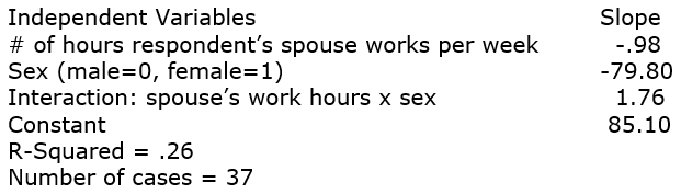 Calculate predicted hours of work for:
a man whose spouse works 20 hours per week
a man whose spouse works 60 hours per week
a woman whose spouse works 20 hours per week
a woman whose spouse works 60 hours per week
Then tell the story going on here.
Dependent Variable: # of hours respondent works per week
Calculate predicted hours of work for:a man whose spouse works 20 hours per week
a man whose spouse works 60 hours per week
a woman whose spouse works 20 hours per week
a woman whose spouse works 60 hours per week
Then tell the story going on here.
Question
We are interested in whether or not education's effect on occupational prestige is the same for whites and blacks. Here is a regression model using GSS2008 data, those aged 18-49. In the 2008GSS, occupational prestige scores ranged from 17 (very low prestige occupation) to 86 (very high prestige occupation).
Dependent Variable: Respondent's Occupational Prestige Score
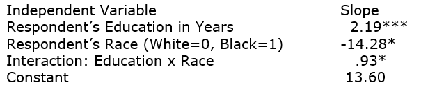 R-squared = .23
n = 908
Predict occupational prestige scores for:
A white person with 8 years of education
A white person with 22 years of education
A black person with 8 years of education
A black person with 22 years of education
Then, interpret the overall story here.
Dependent Variable: Respondent's Occupational Prestige Score
R-squared = .23n = 908
Predict occupational prestige scores for:
A white person with 8 years of education
A white person with 22 years of education
A black person with 8 years of education
A black person with 22 years of education
Then, interpret the overall story here.
Question
We are interested in whether or not education's effect on age at first marriage is the same for men and women. Here is a regression model using GSS2006 data.
Dependent Variable: Age at First Marriage
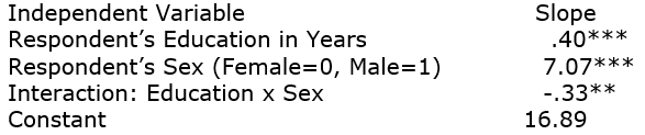 R-squared = .07
n = 1159
Predict age at first marriage for:
A man with 8 years of education
A man with 22 years of education
A woman with 8 years of education
A woman with 22 years of education
Then, interpret the overall story here.
Dependent Variable: Age at First Marriage
R-squared = .07n = 1159
Predict age at first marriage for:
A man with 8 years of education
A man with 22 years of education
A woman with 8 years of education
A woman with 22 years of education
Then, interpret the overall story here.
Question
We are interested in whether or not education's effect on happiness is the same for whites and blacks. Here is a regression model using GSS2006 data. The dependent variable is an index of happiness where 0 = not happy up to 4 = very happy.
Dependent Variable: Happiness Index
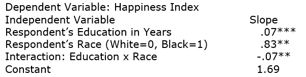 R-squared = .03
n = 1719
Simply by talking about the slopes, describe the effect of education on happiness for both whites and blacks.
Dependent Variable: Happiness Index
R-squared = .03n = 1719
Simply by talking about the slopes, describe the effect of education on happiness for both whites and blacks.
Question
Question
Question
Question
Question

Unlock Deck
Sign up to unlock the cards in this deck!
Unlock Deck
Unlock Deck
1/35
Play
Full screen (f)
Deck 12: Different Slopes for Different Folks: Interaction Effects
1
Complete this analogy: Elaboration is to interaction effects as…
A) regression is to crosstabulation
B) crosstabulation is to regression
C) regression is to standard deviation
D) frequency distribution is to regression
A) regression is to crosstabulation
B) crosstabulation is to regression
C) regression is to standard deviation
D) frequency distribution is to regression
B
2
Which of the following is not a reason to choose interaction over elaboration?
A) The crosstabs tend to be too large
B) It is difficult to control for more than one variable in a crosstab
C) Some of the cells in the crosstabs may have very small frequencies
D) R-squared is better than chi-square
A) The crosstabs tend to be too large
B) It is difficult to control for more than one variable in a crosstab
C) Some of the cells in the crosstabs may have very small frequencies
D) R-squared is better than chi-square
D
3
Let's say we're creating an interaction effect between sex and years of education. If sex is coded Male=0, Female=1, what is the value of the interaction effect for a woman with 16 years of education?
A) 0
B) 16
C) 15
D) 4
A) 0
B) 16
C) 15
D) 4
B
4
Let's say we're creating an interaction effect between sex and years of education. If sex is coded Male=0, Female=1, what is the value of the interaction effect for a man with 16 years of education?
A) 0
B) 16
C) 15
D) 4
A) 0
B) 16
C) 15
D) 4
Unlock Deck
Unlock for access to all 35 flashcards in this deck.
Unlock Deck
k this deck
5
In a regression equation that uses sex (Male=0, Female=1), years of education, and the interaction effect between sex and education, the resulting graphs are two parallel lines. Which of the following must be true?
A) The slope for sex is not statistically significant.
B) The slope for education is not statistically significant.
C) The slope for the interaction effect is not statistically significant.
D) None of the three slopes is statistically significant.
A) The slope for sex is not statistically significant.
B) The slope for education is not statistically significant.
C) The slope for the interaction effect is not statistically significant.
D) None of the three slopes is statistically significant.
Unlock Deck
Unlock for access to all 35 flashcards in this deck.
Unlock Deck
k this deck
6
In a regression equation that uses sex (Male=0, Female=1), the slope for sex has the same exact value as the interaction slope, but a different sign. What best describes the line for women?
A) Its slope will be twice that of the men's slope.
B) Its slope will be half that of the men's slope.
C) It will be completely vertical.
D) It will be completely horizontal.
A) Its slope will be twice that of the men's slope.
B) Its slope will be half that of the men's slope.
C) It will be completely vertical.
D) It will be completely horizontal.
Unlock Deck
Unlock for access to all 35 flashcards in this deck.
Unlock Deck
k this deck
7
Here is a regression model using GSS2006 data. All slopes are statistically significant.
Dependent Variable: Respondent's Age at First Marriage
Which of the following is the best description of the resulting graphed lines?
A) Both lines have positive slopes, but the black line has a steeper slope.
B) Both lines have positive slopes, but the white line has a steeper slope.
C) The white line has a positive slope, the black line has a negative slope.
D) The white line has a negative slope, the black line has a positive slope.
Unlock Deck
Unlock for access to all 35 flashcards in this deck.
Unlock Deck
k this deck
8
Here is a regression model using GSS2008 data, respondents aged 18-35. All slopes are statistically significant:
Dependent Variable: # of Times Respondent Goes to Bar Per Month
Who goes to bars most frequently?
A) Heterosexual men
B) Heterosexual women
C) A gay/bisexual man
D) A lesbian/bisexual woman
Dependent Variable: # of Times Respondent Goes to Bar Per Month
Who goes to bars most frequently?
A) Heterosexual men
B) Heterosexual women
C) A gay/bisexual man
D) A lesbian/bisexual woman
Unlock Deck
Unlock for access to all 35 flashcards in this deck.
Unlock Deck
k this deck
9
What is the most common form of interaction effect presented in Chapter 12?
A) an interaction effect between two ratio-level variables
B) an interaction effect between two dichotomies
C) an interaction effect between a ratio-level variable and a dichotomy
D) an interaction effect between a nominal-level variable and a dichotomy
A) an interaction effect between two ratio-level variables
B) an interaction effect between two dichotomies
C) an interaction effect between a ratio-level variable and a dichotomy
D) an interaction effect between a nominal-level variable and a dichotomy
Unlock Deck
Unlock for access to all 35 flashcards in this deck.
Unlock Deck
k this deck
10
All of the interaction examples in Chapter 12 involve interacting how many parent variables?
A) 2
B) 3
C) 4
D) 5
A) 2
B) 3
C) 4
D) 5
Unlock Deck
Unlock for access to all 35 flashcards in this deck.
Unlock Deck
k this deck
11
In a regression equation that uses sex (Male=0, Female=1), years of education, and the interaction effect between sex and education, all of the resulting slopes are statistically significant. We find that the two parent slopes have positive values and the slope for the interaction effect has a positive value. Which of the following best describes the resulting graphs?
A) The male line starts above the female line and continues to pull away from the female line.
B) The male line starts above the female line, but the female line starts to catch up with the male line.
C) The female line starts above the male line and continues to pull away from the male line.
D) The female line starts above the male line, but the male line starts to catch up with the female line.
Unlock Deck
Unlock for access to all 35 flashcards in this deck.
Unlock Deck
k this deck
12
According to the textbook examples, who is likely to have better health?
A) a poor woman
B) a rich woman
C) a poor man
D) a rich man
A) a poor woman
B) a rich woman
C) a poor man
D) a rich man
Unlock Deck
Unlock for access to all 35 flashcards in this deck.
Unlock Deck
k this deck
13
In a regression equation that uses sex (Male=0, Female=1), years of education, and the interaction effect between sex and education, all of the resulting slopes are statistically significant. We find that the two parent slopes have positive values and the slope for the interaction effect has a negative value half the size of the slope for education. Which of the following best describes the resulting graphs?
A) The male line starts above the female line and continues to pull away from the female line.
B) The male line starts above the female line, but the female line starts to catch up with the male line.
C) The female line starts above the male line and continues to pull away from the male line.
D) The female line starts above the male line, but the male line starts to catch up with the female line.
Unlock Deck
Unlock for access to all 35 flashcards in this deck.
Unlock Deck
k this deck
14
Which statement best describes the relationship between BMI and income?
A) Both men and women experience decreases in income as BMI increases, but women more so.
B) Both men and women experience decreases in income as BMI increases, but men more so.
C) As men's BMI increases, their income goes up, but as women's BMI increases, their income goes down.
D) As women's BMI increases, their income goes up, but as men's BMI increases, their income goes down.
Unlock Deck
Unlock for access to all 35 flashcards in this deck.
Unlock Deck
k this deck
15
In Kisida, Greene, and Bowen's research on art museums, what was the name of the art museum they studied?
A) Crystal Bridges
B) Heather Meadows
C) Amber Towers
D) Whitney Modern
A) Crystal Bridges
B) Heather Meadows
C) Amber Towers
D) Whitney Modern
Unlock Deck
Unlock for access to all 35 flashcards in this deck.
Unlock Deck
k this deck
16
What combination of methods did Kisida, Greene, and Bowen use in their research on art museums?
A) survey research and content analysis
B) survey research and experimentation
C) content analysis and experimentation
D) content analysis and analysis of census data
A) survey research and content analysis
B) survey research and experimentation
C) content analysis and experimentation
D) content analysis and analysis of census data
Unlock Deck
Unlock for access to all 35 flashcards in this deck.
Unlock Deck
k this deck
17
What behavioral measure did Kisida, Greene, and Bowen use?
A) whether or not the student used a coupon to see a special art exhibit
B) whether or not the student asked a question during the museum tour
C) whether or not the student told their parents about their museum tour
D) whether or not the student passed an art quiz after their museum tour
A) whether or not the student used a coupon to see a special art exhibit
B) whether or not the student asked a question during the museum tour
C) whether or not the student told their parents about their museum tour
D) whether or not the student passed an art quiz after their museum tour
Unlock Deck
Unlock for access to all 35 flashcards in this deck.
Unlock Deck
k this deck
18
According to Kisida, Greene, and Bowen's research on art museums, which type of student was most likely to benefit from attending the museum program?
A) a student who previously did no cultural activities and who went to a school with a low percentage of free/reduced lunches.
B) a student who previously did several cultural activities and who went to a school with a low percentage of free/reduced lunches.
C) a student who previously did no cultural activities and who went to a school with a high percentage of free/reduced lunches.
D) a student who previously did several cultural activities and who went to a school with a high percentage of free/reduced lunches.
Unlock Deck
Unlock for access to all 35 flashcards in this deck.
Unlock Deck
k this deck
19
Which dataset did Glavin, Schieman, and Reid use for their research on work?
A) The General Social Survey
B) The National Survey of Families and Households
C) The Panel Study of Income Dynamics
D) The Work, Stress, and Health Survey
A) The General Social Survey
B) The National Survey of Families and Households
C) The Panel Study of Income Dynamics
D) The Work, Stress, and Health Survey
Unlock Deck
Unlock for access to all 35 flashcards in this deck.
Unlock Deck
k this deck
20
In Glavin, Schieman, and Reid's research on work, what is the dependent variable?
A) sleep deprivation
B) hours of work
C) hours to relax
D) guilt
A) sleep deprivation
B) hours of work
C) hours to relax
D) guilt
Unlock Deck
Unlock for access to all 35 flashcards in this deck.
Unlock Deck
k this deck
21
In Glavin, Schieman, and Reid's research, how did they measure work contact?
A) counting work-related phone calls the respondent received when phone was located in the home
B) asking the respondent's boss how available the respondent typically was after work hours
C) checking the respondent's email log
D) asking the respondent how often work demands happen after normal work hours
Unlock Deck
Unlock for access to all 35 flashcards in this deck.
Unlock Deck
k this deck
22
Which of the following best describes the findings of Glavin, Schieman, and Reid?
A) Work contact outside of work raises the guilt level of both men and women.
B) Work contact outside of work raises the guilt level of men, but not women.
C) Work contact outside of work lowers the guilt level of men, but raises the guilt level of women.
D) Work contact outside of work has no effect on men's and women's guilt.
Unlock Deck
Unlock for access to all 35 flashcards in this deck.
Unlock Deck
k this deck
23
In SPSS, we want to create an interaction effect with RACEWB (a dichotomous race variable) and EDUC (years of education). What is the proper compute command?
A) RACEWB + EDUC
B) RACEWB / EDUC
C) RACEWB * EDUC
D) (RACEWB)(EDUC)
A) RACEWB + EDUC
B) RACEWB / EDUC
C) RACEWB * EDUC
D) (RACEWB)(EDUC)
Unlock Deck
Unlock for access to all 35 flashcards in this deck.
Unlock Deck
k this deck
24
Here is a box of SPSS output:
What is the correct equation to use to create examples?
A) ATTEND = 1.41 +1.54(SEX) +.01(EDUC) -.08(SEX)(EDUC)
B) ATTEND = 1.41 +1.54(SEX) -.08(SEX)(EDUC)
C) ATTEND = 1.41 +.32(SEX) +.01(EDUC) -.22(SEX)(EDUC)
D) ATTEND = 1.41 +1.54(SEX) +.01(EDUC)
What is the correct equation to use to create examples?
A) ATTEND = 1.41 +1.54(SEX) +.01(EDUC) -.08(SEX)(EDUC)
B) ATTEND = 1.41 +1.54(SEX) -.08(SEX)(EDUC)
C) ATTEND = 1.41 +.32(SEX) +.01(EDUC) -.22(SEX)(EDUC)
D) ATTEND = 1.41 +1.54(SEX) +.01(EDUC)
Unlock Deck
Unlock for access to all 35 flashcards in this deck.
Unlock Deck
k this deck
25
Which type of interaction did not appear in Chapter 12?
A) The interaction between two dichotomies
B) The interaction between a dichotomy and a set of reference-group variables
C) The interaction between two ratio-level variables
D) All of these appeared in Chapter 12
A) The interaction between two dichotomies
B) The interaction between a dichotomy and a set of reference-group variables
C) The interaction between two ratio-level variables
D) All of these appeared in Chapter 12
Unlock Deck
Unlock for access to all 35 flashcards in this deck.
Unlock Deck
k this deck
26
Describe the typical format of a research question that would lead you to using interaction effects.
Unlock Deck
Unlock for access to all 35 flashcards in this deck.
Unlock Deck
k this deck
27
Using GSS2006 data, only the African American respondents, we see if how many hours a respondent's spouse works affects how much the respondent works. Here is the model:
Dependent Variable: # of hours respondent works per week
Calculate predicted hours of work for:
a man whose spouse works 20 hours per week
a man whose spouse works 60 hours per week
a woman whose spouse works 20 hours per week
a woman whose spouse works 60 hours per week
Then tell the story going on here.
Dependent Variable: # of hours respondent works per week
Calculate predicted hours of work for:a man whose spouse works 20 hours per week
a man whose spouse works 60 hours per week
a woman whose spouse works 20 hours per week
a woman whose spouse works 60 hours per week
Then tell the story going on here.
Unlock Deck
Unlock for access to all 35 flashcards in this deck.
Unlock Deck
k this deck
28
We are interested in whether or not education's effect on occupational prestige is the same for whites and blacks. Here is a regression model using GSS2008 data, those aged 18-49. In the 2008GSS, occupational prestige scores ranged from 17 (very low prestige occupation) to 86 (very high prestige occupation).
Dependent Variable: Respondent's Occupational Prestige Score
R-squared = .23
n = 908
Predict occupational prestige scores for:
A white person with 8 years of education
A white person with 22 years of education
A black person with 8 years of education
A black person with 22 years of education
Then, interpret the overall story here.
Dependent Variable: Respondent's Occupational Prestige Score
R-squared = .23n = 908
Predict occupational prestige scores for:
A white person with 8 years of education
A white person with 22 years of education
A black person with 8 years of education
A black person with 22 years of education
Then, interpret the overall story here.
Unlock Deck
Unlock for access to all 35 flashcards in this deck.
Unlock Deck
k this deck
29
We are interested in whether or not education's effect on age at first marriage is the same for men and women. Here is a regression model using GSS2006 data.
Dependent Variable: Age at First Marriage
R-squared = .07
n = 1159
Predict age at first marriage for:
A man with 8 years of education
A man with 22 years of education
A woman with 8 years of education
A woman with 22 years of education
Then, interpret the overall story here.
Dependent Variable: Age at First Marriage
R-squared = .07n = 1159
Predict age at first marriage for:
A man with 8 years of education
A man with 22 years of education
A woman with 8 years of education
A woman with 22 years of education
Then, interpret the overall story here.
Unlock Deck
Unlock for access to all 35 flashcards in this deck.
Unlock Deck
k this deck
30
We are interested in whether or not education's effect on happiness is the same for whites and blacks. Here is a regression model using GSS2006 data. The dependent variable is an index of happiness where 0 = not happy up to 4 = very happy.
Dependent Variable: Happiness Index
R-squared = .03
n = 1719
Simply by talking about the slopes, describe the effect of education on happiness for both whites and blacks.
Dependent Variable: Happiness Index
R-squared = .03n = 1719
Simply by talking about the slopes, describe the effect of education on happiness for both whites and blacks.
Unlock Deck
Unlock for access to all 35 flashcards in this deck.
Unlock Deck
k this deck
31
You hypothesize that, among men and women who have few years of education, men have higher incomes than women, but for every year of education, women catch up a bit to men, so that by the time you're looking at highly educated men and women, women have higher incomes than men.
Without talking about specific numbers, describe what the direction of the slopes for sex, years of education, and the interaction between sex and years of education would look like. Assume that the sex variable is coded M=0, F=1.
Without talking about specific numbers, describe what the direction of the slopes for sex, years of education, and the interaction between sex and years of education would look like. Assume that the sex variable is coded M=0, F=1.
Unlock Deck
Unlock for access to all 35 flashcards in this deck.
Unlock Deck
k this deck
32
You hypothesize that, among men and women who have few years of education, men have higher slightly higher incomes than women, and that for every year of education, men pull even further ahead, so that by the time you're looking at highly educated men and women, men have much higher incomes than women. Without talking about specific numbers, describe what the direction of the slopes for sex, years of education, and the interaction between sex and years of education would look like. Assume that the sex variable is coded M=0, F=1.
Unlock Deck
Unlock for access to all 35 flashcards in this deck.
Unlock Deck
k this deck
33
You hypothesize that education affects the number of children a person has, but you think that this effect is different for men and women: among men, you expect a positive effect, but among women, you expect a negative effect. You expect that women with little education will have more children than men with little education, and you expect that women with lots of education will have fewer children than men with lots of education. Without talking about specific numbers, describe what the direction of the slopes for sex, years of education, and the interaction between sex and years of education would look like. Assume that the sex variable is coded M=0, F=1.
Unlock Deck
Unlock for access to all 35 flashcards in this deck.
Unlock Deck
k this deck
34
You hypothesize that, among women, education has a negative effect on the number of times per month they attend religious services, but that among men, there is no effect at all. You expect that women with little education will attend religious services more than men attend. Without talking about specific numbers, describe what the direction of the slopes for sex, years of education, and the interaction between sex and years of education would look like. Assume that the sex variable is coded M=1, F=0.
Unlock Deck
Unlock for access to all 35 flashcards in this deck.
Unlock Deck
k this deck
35
Describe how Glavin, Schieman, and Reid's article used interaction effects. What did they interact? What did they find?
Unlock Deck
Unlock for access to all 35 flashcards in this deck.
Unlock Deck
k this deck
Unlock Deck
Unlock for access to all 35 flashcards in this deck.


