Deck 16: Government Regulation of Business
Full screen (f)
Question
The cost and demand conditions for residential water consumption are shown below. If there are 450,000 residential water customers, then develop an optimal two-part pricing scheme
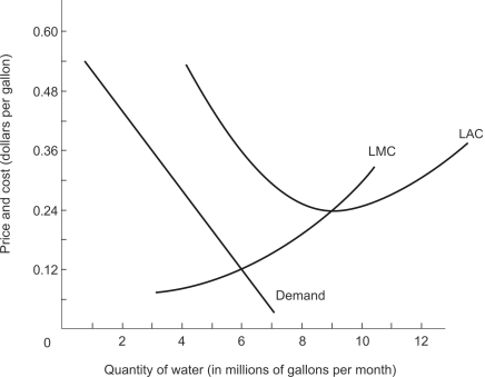
-The optimal usage fee to charge is _______ per gallon of water.
A) $0.12
B) $0.18
C) $0.24
D) $0.30
E) $0.36
-The optimal usage fee to charge is _______ per gallon of water.
A) $0.12
B) $0.18
C) $0.24
D) $0.30
E) $0.36
Question
The cost and demand conditions for residential water consumption are shown below. If there are 450,000 residential water customers, then develop an optimal two-part pricing scheme
-At the optimal user fee in the previous question, the water utility company will lose _______ per month.
A) $0
B) $1,440,000
C) $1,680,000
D) $2,400,000
E) $3,242,500
-At the optimal user fee in the previous question, the water utility company will lose _______ per month.
A) $0
B) $1,440,000
C) $1,680,000
D) $2,400,000
E) $3,242,500
Question
The cost and demand conditions for residential water consumption are shown below. If there are 450,000 residential water customers, then develop an optimal two-part pricing scheme
-The optimal monthly access charge per household is _______ per residence (per month).
A) $0.12
B) $0.18
C) $12
D) $24
E) $32
-The optimal monthly access charge per household is _______ per residence (per month).
A) $0.12
B) $0.18
C) $12
D) $24
E) $32
Question
The figure below shows the result of a price fixing scheme that raised price above competitive levels at point C to a price of $15 at point M.
?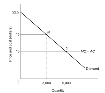
-By forming this price-fixing cartel, producers gained $__________ of producer surplus, while consumers lost $__________ of consumer surplus.
A) $15,000; $10,000
B) $15,000; $20,000
C) $20,000; $10,000
D) $20,000; $5,000
?
-By forming this price-fixing cartel, producers gained $__________ of producer surplus, while consumers lost $__________ of consumer surplus.
A) $15,000; $10,000
B) $15,000; $20,000
C) $20,000; $10,000
D) $20,000; $5,000
Question
refer to the following information:
A municipal water utility employs quasi-fixed capital inputs-are the water treatment plant and distribution lines to homes-to supply water to 20,000 households in the community it serves. The figure below shows the cost structure of this utility for various levels of water service. Quantity of water consumption is measured in 1,000-gallon units per month. AQFC is the average quasi-fixed cost curve, and LAC is long-run average cost. Long-run marginal cost, LMC, is constant and equal to $4 per 1,000-gallon unit. The inverse demand equation is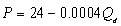 .
.
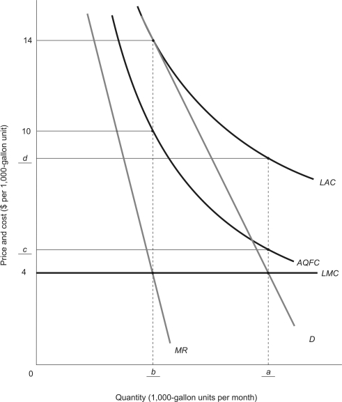
-The value in blank a in the figure is ____.
A) 40,000
B) 45,000
C) 50,000
D) 55,000
E) none of the above
A municipal water utility employs quasi-fixed capital inputs-are the water treatment plant and distribution lines to homes-to supply water to 20,000 households in the community it serves. The figure below shows the cost structure of this utility for various levels of water service. Quantity of water consumption is measured in 1,000-gallon units per month. AQFC is the average quasi-fixed cost curve, and LAC is long-run average cost. Long-run marginal cost, LMC, is constant and equal to $4 per 1,000-gallon unit. The inverse demand equation is
.-The value in blank a in the figure is ____.
A) 40,000
B) 45,000
C) 50,000
D) 55,000
E) none of the above
Question
refer to the following information:
A municipal water utility employs quasi-fixed capital inputs-are the water treatment plant and distribution lines to homes-to supply water to 20,000 households in the community it serves. The figure below shows the cost structure of this utility for various levels of water service. Quantity of water consumption is measured in 1,000-gallon units per month. AQFC is the average quasi-fixed cost curve, and LAC is long-run average cost. Long-run marginal cost, LMC, is constant and equal to $4 per 1,000-gallon unit. The inverse demand equation is .
-The value in blank b in the figure is ____.
A) 22,500
B) 25,000
C) 27,500
D) 30,000
E) none of the above
A municipal water utility employs quasi-fixed capital inputs-are the water treatment plant and distribution lines to homes-to supply water to 20,000 households in the community it serves. The figure below shows the cost structure of this utility for various levels of water service. Quantity of water consumption is measured in 1,000-gallon units per month. AQFC is the average quasi-fixed cost curve, and LAC is long-run average cost. Long-run marginal cost, LMC, is constant and equal to $4 per 1,000-gallon unit. The inverse demand equation is
.-The value in blank b in the figure is ____.
A) 22,500
B) 25,000
C) 27,500
D) 30,000
E) none of the above
Question
refer to the following information:
A municipal water utility employs quasi-fixed capital inputs-are the water treatment plant and distribution lines to homes-to supply water to 20,000 households in the community it serves. The figure below shows the cost structure of this utility for various levels of water service. Quantity of water consumption is measured in 1,000-gallon units per month. AQFC is the average quasi-fixed cost curve, and LAC is long-run average cost. Long-run marginal cost, LMC, is constant and equal to $4 per 1,000-gallon unit. The inverse demand equation is .
-The value in blank c in the figure is ____.
A) $4.65
B) $4.75
C) $4.80
D) $5.50
E) none of the above
A municipal water utility employs quasi-fixed capital inputs-are the water treatment plant and distribution lines to homes-to supply water to 20,000 households in the community it serves. The figure below shows the cost structure of this utility for various levels of water service. Quantity of water consumption is measured in 1,000-gallon units per month. AQFC is the average quasi-fixed cost curve, and LAC is long-run average cost. Long-run marginal cost, LMC, is constant and equal to $4 per 1,000-gallon unit. The inverse demand equation is
.-The value in blank c in the figure is ____.
A) $4.65
B) $4.75
C) $4.80
D) $5.50
E) none of the above
Question
refer to the following information:
A municipal water utility employs quasi-fixed capital inputs-are the water treatment plant and distribution lines to homes-to supply water to 20,000 households in the community it serves. The figure below shows the cost structure of this utility for various levels of water service. Quantity of water consumption is measured in 1,000-gallon units per month. AQFC is the average quasi-fixed cost curve, and LAC is long-run average cost. Long-run marginal cost, LMC, is constant and equal to $4 per 1,000-gallon unit. The inverse demand equation is .
-The value in blank d in the figure is ____.
A) 6.50
B) 7.50
C) 8.00
D) 9.50
E) none of the above
A municipal water utility employs quasi-fixed capital inputs-are the water treatment plant and distribution lines to homes-to supply water to 20,000 households in the community it serves. The figure below shows the cost structure of this utility for various levels of water service. Quantity of water consumption is measured in 1,000-gallon units per month. AQFC is the average quasi-fixed cost curve, and LAC is long-run average cost. Long-run marginal cost, LMC, is constant and equal to $4 per 1,000-gallon unit. The inverse demand equation is
.-The value in blank d in the figure is ____.
A) 6.50
B) 7.50
C) 8.00
D) 9.50
E) none of the above
Question
refer to the following information:
A municipal water utility employs quasi-fixed capital inputs-are the water treatment plant and distribution lines to homes-to supply water to 20,000 households in the community it serves. The figure below shows the cost structure of this utility for various levels of water service. Quantity of water consumption is measured in 1,000-gallon units per month. AQFC is the average quasi-fixed cost curve, and LAC is long-run average cost. Long-run marginal cost, LMC, is constant and equal to $4 per 1,000-gallon unit. The inverse demand equation is .
-Quasi-fixed capital inputs cost per month is $____.
A) 150,000
B) 200,000
C) 250,000
D) 300,000
E) 350,000
A municipal water utility employs quasi-fixed capital inputs-are the water treatment plant and distribution lines to homes-to supply water to 20,000 households in the community it serves. The figure below shows the cost structure of this utility for various levels of water service. Quantity of water consumption is measured in 1,000-gallon units per month. AQFC is the average quasi-fixed cost curve, and LAC is long-run average cost. Long-run marginal cost, LMC, is constant and equal to $4 per 1,000-gallon unit. The inverse demand equation is
.-Quasi-fixed capital inputs cost per month is $____.
A) 150,000
B) 200,000
C) 250,000
D) 300,000
E) 350,000
Question
refer to the following information:
A municipal water utility employs quasi-fixed capital inputs-are the water treatment plant and distribution lines to homes-to supply water to 20,000 households in the community it serves. The figure below shows the cost structure of this utility for various levels of water service. Quantity of water consumption is measured in 1,000-gallon units per month. AQFC is the average quasi-fixed cost curve, and LAC is long-run average cost. Long-run marginal cost, LMC, is constant and equal to $4 per 1,000-gallon unit. The inverse demand equation is .
-The price and output of water that maximize social surplus are _____ and _____, respectively.
A) $9.00; 50,000
B) $4.00; 25,000
C) $4.00; 50,000
D) none of the above
A municipal water utility employs quasi-fixed capital inputs-are the water treatment plant and distribution lines to homes-to supply water to 20,000 households in the community it serves. The figure below shows the cost structure of this utility for various levels of water service. Quantity of water consumption is measured in 1,000-gallon units per month. AQFC is the average quasi-fixed cost curve, and LAC is long-run average cost. Long-run marginal cost, LMC, is constant and equal to $4 per 1,000-gallon unit. The inverse demand equation is
.-The price and output of water that maximize social surplus are _____ and _____, respectively.
A) $9.00; 50,000
B) $4.00; 25,000
C) $4.00; 50,000
D) none of the above
Question
refer to the following information:
A municipal water utility employs quasi-fixed capital inputs-are the water treatment plant and distribution lines to homes-to supply water to 20,000 households in the community it serves. The figure below shows the cost structure of this utility for various levels of water service. Quantity of water consumption is measured in 1,000-gallon units per month. AQFC is the average quasi-fixed cost curve, and LAC is long-run average cost. Long-run marginal cost, LMC, is constant and equal to $4 per 1,000-gallon unit. The inverse demand equation is .
-If the Public Service Commission undertakes second-best pricing, the price and output of water are __________ and _________, respectively.
A) $2.00; 55,000
B) $9.00; 50,000
C) $2.50; 27,500
D) $9.50; 55,000
E) none of the above
A municipal water utility employs quasi-fixed capital inputs-are the water treatment plant and distribution lines to homes-to supply water to 20,000 households in the community it serves. The figure below shows the cost structure of this utility for various levels of water service. Quantity of water consumption is measured in 1,000-gallon units per month. AQFC is the average quasi-fixed cost curve, and LAC is long-run average cost. Long-run marginal cost, LMC, is constant and equal to $4 per 1,000-gallon unit. The inverse demand equation is
.-If the Public Service Commission undertakes second-best pricing, the price and output of water are __________ and _________, respectively.
A) $2.00; 55,000
B) $9.00; 50,000
C) $2.50; 27,500
D) $9.50; 55,000
E) none of the above
Question
refer to the following information:
A municipal water utility employs quasi-fixed capital inputs-are the water treatment plant and distribution lines to homes-to supply water to 20,000 households in the community it serves. The figure below shows the cost structure of this utility for various levels of water service. Quantity of water consumption is measured in 1,000-gallon units per month. AQFC is the average quasi-fixed cost curve, and LAC is long-run average cost. Long-run marginal cost, LMC, is constant and equal to $4 per 1,000-gallon unit. The inverse demand equation is .
-Second-best pricing does not achieve social economic efficiency because there is a dead weight loss of
A) $125,000.
B) $150,000.
C) $200,000.
D) $250,000
E) $300,000
A municipal water utility employs quasi-fixed capital inputs-are the water treatment plant and distribution lines to homes-to supply water to 20,000 households in the community it serves. The figure below shows the cost structure of this utility for various levels of water service. Quantity of water consumption is measured in 1,000-gallon units per month. AQFC is the average quasi-fixed cost curve, and LAC is long-run average cost. Long-run marginal cost, LMC, is constant and equal to $4 per 1,000-gallon unit. The inverse demand equation is
.-Second-best pricing does not achieve social economic efficiency because there is a dead weight loss of
A) $125,000.
B) $150,000.
C) $200,000.
D) $250,000
E) $300,000
Question
Use the figure below, which shows the linear demand and constant cost conditions facing a firm with a high barrier to entry,
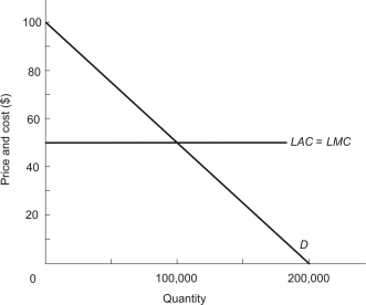
-The firm will earn economic profit of $______.
A) $500,000
B) $750,000
C) $1,000,000
D) $1,500,000
-The firm will earn economic profit of $______.
A) $500,000
B) $750,000
C) $1,000,000
D) $1,500,000
Question
Use the figure below, which shows the linear demand and constant cost conditions facing a firm with a high barrier to entry,
-$_________ the deadweight loss is caused by the market power created by the high entry barrier
A) $750,000
B) $1,000,000
C) $1,500,000
D) $2,000,000
-$_________ the deadweight loss is caused by the market power created by the high entry barrier
A) $750,000
B) $1,000,000
C) $1,500,000
D) $2,000,000
Question
Question
Question
Question
Question
Question
Question
Question
Question
Question
Question
The market for bagels in San Francisco is perfectly competitive. Presently, the daily demand for bagels in San Francisco is Qd = 15,000 - 5,000P, and the supply of bagels is Qs = 10,000P, where P is the price of bagels and quantities Qd and Qs, respectively, are the number of bagels bought and sold each day. The figure below shows the demand and supply curves for bagels in San Francisco.

-The competitive equilibrium price of bagels in San Francisco is $_______ and the equilibrium quantity is ___________ bagels per day.
-The competitive equilibrium price of bagels in San Francisco is $_______ and the equilibrium quantity is ___________ bagels per day.
Question
The market for bagels in San Francisco is perfectly competitive. Presently, the daily demand for bagels in San Francisco is Qd = 15,000 - 5,000P, and the supply of bagels is Qs = 10,000P, where P is the price of bagels and quantities Qd and Qs, respectively, are the number of bagels bought and sold each day. The figure below shows the demand and supply curves for bagels in San Francisco.
-The consumer surplus for the 5,000th bagel is $_______. The producer surplus for the 5,000th bagel is $_______.
-The consumer surplus for the 5,000th bagel is $_______. The producer surplus for the 5,000th bagel is $_______.
Question
The market for bagels in San Francisco is perfectly competitive. Presently, the daily demand for bagels in San Francisco is Qd = 15,000 - 5,000P, and the supply of bagels is Qs = 10,000P, where P is the price of bagels and quantities Qd and Qs, respectively, are the number of bagels bought and sold each day. The figure below shows the demand and supply curves for bagels in San Francisco.
-In competitive equilibrium in the San Francisco bagel market, total consumer surplus is $__________ and total producer surplus is $_________. Social surplus is $__________.
Now suppose Einstein Bagels buys every other bagel store in town and forms a bagel monopoly in San Francisco.
-In competitive equilibrium in the San Francisco bagel market, total consumer surplus is $__________ and total producer surplus is $_________. Social surplus is $__________.
Now suppose Einstein Bagels buys every other bagel store in town and forms a bagel monopoly in San Francisco.
Question
The market for bagels in San Francisco is perfectly competitive. Presently, the daily demand for bagels in San Francisco is Qd = 15,000 - 5,000P, and the supply of bagels is Qs = 10,000P, where P is the price of bagels and quantities Qd and Qs, respectively, are the number of bagels bought and sold each day. The figure below shows the demand and supply curves for bagels in San Francisco.
-The monopoly price of bagels is $__________ and the number of bagels bought and sold daily is ____________ bagels per day under monopoly.
-The monopoly price of bagels is $__________ and the number of bagels bought and sold daily is ____________ bagels per day under monopoly.
Question
The market for bagels in San Francisco is perfectly competitive. Presently, the daily demand for bagels in San Francisco is Qd = 15,000 - 5,000P, and the supply of bagels is Qs = 10,000P, where P is the price of bagels and quantities Qd and Qs, respectively, are the number of bagels bought and sold each day. The figure below shows the demand and supply curves for bagels in San Francisco.
-The deadweight loss due to the bagel monopoly in San Francisco is $______________.
-The deadweight loss due to the bagel monopoly in San Francisco is $______________.

Unlock Deck
Sign up to unlock the cards in this deck!
Unlock Deck
Unlock Deck
1/29
Play
Full screen (f)
Deck 16: Government Regulation of Business
1
The cost and demand conditions for residential water consumption are shown below. If there are 450,000 residential water customers, then develop an optimal two-part pricing scheme
-The optimal usage fee to charge is _______ per gallon of water.
A) $0.12
B) $0.18
C) $0.24
D) $0.30
E) $0.36
-The optimal usage fee to charge is _______ per gallon of water.
A) $0.12
B) $0.18
C) $0.24
D) $0.30
E) $0.36
$0.12
2
The cost and demand conditions for residential water consumption are shown below. If there are 450,000 residential water customers, then develop an optimal two-part pricing scheme
-At the optimal user fee in the previous question, the water utility company will lose _______ per month.
A) $0
B) $1,440,000
C) $1,680,000
D) $2,400,000
E) $3,242,500
-At the optimal user fee in the previous question, the water utility company will lose _______ per month.
A) $0
B) $1,440,000
C) $1,680,000
D) $2,400,000
E) $3,242,500
$1,440,000
3
The cost and demand conditions for residential water consumption are shown below. If there are 450,000 residential water customers, then develop an optimal two-part pricing scheme
-The optimal monthly access charge per household is _______ per residence (per month).
A) $0.12
B) $0.18
C) $12
D) $24
E) $32
-The optimal monthly access charge per household is _______ per residence (per month).
A) $0.12
B) $0.18
C) $12
D) $24
E) $32
$32
4
The figure below shows the result of a price fixing scheme that raised price above competitive levels at point C to a price of $15 at point M.
?
-By forming this price-fixing cartel, producers gained $__________ of producer surplus, while consumers lost $__________ of consumer surplus.
A) $15,000; $10,000
B) $15,000; $20,000
C) $20,000; $10,000
D) $20,000; $5,000
?
-By forming this price-fixing cartel, producers gained $__________ of producer surplus, while consumers lost $__________ of consumer surplus.
A) $15,000; $10,000
B) $15,000; $20,000
C) $20,000; $10,000
D) $20,000; $5,000
Unlock Deck
Unlock for access to all 29 flashcards in this deck.
Unlock Deck
k this deck
5
refer to the following information:
A municipal water utility employs quasi-fixed capital inputs-are the water treatment plant and distribution lines to homes-to supply water to 20,000 households in the community it serves. The figure below shows the cost structure of this utility for various levels of water service. Quantity of water consumption is measured in 1,000-gallon units per month. AQFC is the average quasi-fixed cost curve, and LAC is long-run average cost. Long-run marginal cost, LMC, is constant and equal to $4 per 1,000-gallon unit. The inverse demand equation is .
-The value in blank a in the figure is ____.
A) 40,000
B) 45,000
C) 50,000
D) 55,000
E) none of the above
A municipal water utility employs quasi-fixed capital inputs-are the water treatment plant and distribution lines to homes-to supply water to 20,000 households in the community it serves. The figure below shows the cost structure of this utility for various levels of water service. Quantity of water consumption is measured in 1,000-gallon units per month. AQFC is the average quasi-fixed cost curve, and LAC is long-run average cost. Long-run marginal cost, LMC, is constant and equal to $4 per 1,000-gallon unit. The inverse demand equation is
.-The value in blank a in the figure is ____.
A) 40,000
B) 45,000
C) 50,000
D) 55,000
E) none of the above
Unlock Deck
Unlock for access to all 29 flashcards in this deck.
Unlock Deck
k this deck
6
refer to the following information:
A municipal water utility employs quasi-fixed capital inputs-are the water treatment plant and distribution lines to homes-to supply water to 20,000 households in the community it serves. The figure below shows the cost structure of this utility for various levels of water service. Quantity of water consumption is measured in 1,000-gallon units per month. AQFC is the average quasi-fixed cost curve, and LAC is long-run average cost. Long-run marginal cost, LMC, is constant and equal to $4 per 1,000-gallon unit. The inverse demand equation is .
-The value in blank b in the figure is ____.
A) 22,500
B) 25,000
C) 27,500
D) 30,000
E) none of the above
A municipal water utility employs quasi-fixed capital inputs-are the water treatment plant and distribution lines to homes-to supply water to 20,000 households in the community it serves. The figure below shows the cost structure of this utility for various levels of water service. Quantity of water consumption is measured in 1,000-gallon units per month. AQFC is the average quasi-fixed cost curve, and LAC is long-run average cost. Long-run marginal cost, LMC, is constant and equal to $4 per 1,000-gallon unit. The inverse demand equation is
.-The value in blank b in the figure is ____.
A) 22,500
B) 25,000
C) 27,500
D) 30,000
E) none of the above
Unlock Deck
Unlock for access to all 29 flashcards in this deck.
Unlock Deck
k this deck
7
refer to the following information:
A municipal water utility employs quasi-fixed capital inputs-are the water treatment plant and distribution lines to homes-to supply water to 20,000 households in the community it serves. The figure below shows the cost structure of this utility for various levels of water service. Quantity of water consumption is measured in 1,000-gallon units per month. AQFC is the average quasi-fixed cost curve, and LAC is long-run average cost. Long-run marginal cost, LMC, is constant and equal to $4 per 1,000-gallon unit. The inverse demand equation is .
-The value in blank c in the figure is ____.
A) $4.65
B) $4.75
C) $4.80
D) $5.50
E) none of the above
A municipal water utility employs quasi-fixed capital inputs-are the water treatment plant and distribution lines to homes-to supply water to 20,000 households in the community it serves. The figure below shows the cost structure of this utility for various levels of water service. Quantity of water consumption is measured in 1,000-gallon units per month. AQFC is the average quasi-fixed cost curve, and LAC is long-run average cost. Long-run marginal cost, LMC, is constant and equal to $4 per 1,000-gallon unit. The inverse demand equation is
.-The value in blank c in the figure is ____.
A) $4.65
B) $4.75
C) $4.80
D) $5.50
E) none of the above
Unlock Deck
Unlock for access to all 29 flashcards in this deck.
Unlock Deck
k this deck
8
refer to the following information:
A municipal water utility employs quasi-fixed capital inputs-are the water treatment plant and distribution lines to homes-to supply water to 20,000 households in the community it serves. The figure below shows the cost structure of this utility for various levels of water service. Quantity of water consumption is measured in 1,000-gallon units per month. AQFC is the average quasi-fixed cost curve, and LAC is long-run average cost. Long-run marginal cost, LMC, is constant and equal to $4 per 1,000-gallon unit. The inverse demand equation is .
-The value in blank d in the figure is ____.
A) 6.50
B) 7.50
C) 8.00
D) 9.50
E) none of the above
A municipal water utility employs quasi-fixed capital inputs-are the water treatment plant and distribution lines to homes-to supply water to 20,000 households in the community it serves. The figure below shows the cost structure of this utility for various levels of water service. Quantity of water consumption is measured in 1,000-gallon units per month. AQFC is the average quasi-fixed cost curve, and LAC is long-run average cost. Long-run marginal cost, LMC, is constant and equal to $4 per 1,000-gallon unit. The inverse demand equation is
.-The value in blank d in the figure is ____.
A) 6.50
B) 7.50
C) 8.00
D) 9.50
E) none of the above
Unlock Deck
Unlock for access to all 29 flashcards in this deck.
Unlock Deck
k this deck
9
refer to the following information:
A municipal water utility employs quasi-fixed capital inputs-are the water treatment plant and distribution lines to homes-to supply water to 20,000 households in the community it serves. The figure below shows the cost structure of this utility for various levels of water service. Quantity of water consumption is measured in 1,000-gallon units per month. AQFC is the average quasi-fixed cost curve, and LAC is long-run average cost. Long-run marginal cost, LMC, is constant and equal to $4 per 1,000-gallon unit. The inverse demand equation is .
-Quasi-fixed capital inputs cost per month is $____.
A) 150,000
B) 200,000
C) 250,000
D) 300,000
E) 350,000
A municipal water utility employs quasi-fixed capital inputs-are the water treatment plant and distribution lines to homes-to supply water to 20,000 households in the community it serves. The figure below shows the cost structure of this utility for various levels of water service. Quantity of water consumption is measured in 1,000-gallon units per month. AQFC is the average quasi-fixed cost curve, and LAC is long-run average cost. Long-run marginal cost, LMC, is constant and equal to $4 per 1,000-gallon unit. The inverse demand equation is
.-Quasi-fixed capital inputs cost per month is $____.
A) 150,000
B) 200,000
C) 250,000
D) 300,000
E) 350,000
Unlock Deck
Unlock for access to all 29 flashcards in this deck.
Unlock Deck
k this deck
10
refer to the following information:
A municipal water utility employs quasi-fixed capital inputs-are the water treatment plant and distribution lines to homes-to supply water to 20,000 households in the community it serves. The figure below shows the cost structure of this utility for various levels of water service. Quantity of water consumption is measured in 1,000-gallon units per month. AQFC is the average quasi-fixed cost curve, and LAC is long-run average cost. Long-run marginal cost, LMC, is constant and equal to $4 per 1,000-gallon unit. The inverse demand equation is .
-The price and output of water that maximize social surplus are _____ and _____, respectively.
A) $9.00; 50,000
B) $4.00; 25,000
C) $4.00; 50,000
D) none of the above
A municipal water utility employs quasi-fixed capital inputs-are the water treatment plant and distribution lines to homes-to supply water to 20,000 households in the community it serves. The figure below shows the cost structure of this utility for various levels of water service. Quantity of water consumption is measured in 1,000-gallon units per month. AQFC is the average quasi-fixed cost curve, and LAC is long-run average cost. Long-run marginal cost, LMC, is constant and equal to $4 per 1,000-gallon unit. The inverse demand equation is
.-The price and output of water that maximize social surplus are _____ and _____, respectively.
A) $9.00; 50,000
B) $4.00; 25,000
C) $4.00; 50,000
D) none of the above
Unlock Deck
Unlock for access to all 29 flashcards in this deck.
Unlock Deck
k this deck
11
refer to the following information:
A municipal water utility employs quasi-fixed capital inputs-are the water treatment plant and distribution lines to homes-to supply water to 20,000 households in the community it serves. The figure below shows the cost structure of this utility for various levels of water service. Quantity of water consumption is measured in 1,000-gallon units per month. AQFC is the average quasi-fixed cost curve, and LAC is long-run average cost. Long-run marginal cost, LMC, is constant and equal to $4 per 1,000-gallon unit. The inverse demand equation is .
-If the Public Service Commission undertakes second-best pricing, the price and output of water are __________ and _________, respectively.
A) $2.00; 55,000
B) $9.00; 50,000
C) $2.50; 27,500
D) $9.50; 55,000
E) none of the above
A municipal water utility employs quasi-fixed capital inputs-are the water treatment plant and distribution lines to homes-to supply water to 20,000 households in the community it serves. The figure below shows the cost structure of this utility for various levels of water service. Quantity of water consumption is measured in 1,000-gallon units per month. AQFC is the average quasi-fixed cost curve, and LAC is long-run average cost. Long-run marginal cost, LMC, is constant and equal to $4 per 1,000-gallon unit. The inverse demand equation is
.-If the Public Service Commission undertakes second-best pricing, the price and output of water are __________ and _________, respectively.
A) $2.00; 55,000
B) $9.00; 50,000
C) $2.50; 27,500
D) $9.50; 55,000
E) none of the above
Unlock Deck
Unlock for access to all 29 flashcards in this deck.
Unlock Deck
k this deck
12
refer to the following information:
A municipal water utility employs quasi-fixed capital inputs-are the water treatment plant and distribution lines to homes-to supply water to 20,000 households in the community it serves. The figure below shows the cost structure of this utility for various levels of water service. Quantity of water consumption is measured in 1,000-gallon units per month. AQFC is the average quasi-fixed cost curve, and LAC is long-run average cost. Long-run marginal cost, LMC, is constant and equal to $4 per 1,000-gallon unit. The inverse demand equation is .
-Second-best pricing does not achieve social economic efficiency because there is a dead weight loss of
A) $125,000.
B) $150,000.
C) $200,000.
D) $250,000
E) $300,000
A municipal water utility employs quasi-fixed capital inputs-are the water treatment plant and distribution lines to homes-to supply water to 20,000 households in the community it serves. The figure below shows the cost structure of this utility for various levels of water service. Quantity of water consumption is measured in 1,000-gallon units per month. AQFC is the average quasi-fixed cost curve, and LAC is long-run average cost. Long-run marginal cost, LMC, is constant and equal to $4 per 1,000-gallon unit. The inverse demand equation is
.-Second-best pricing does not achieve social economic efficiency because there is a dead weight loss of
A) $125,000.
B) $150,000.
C) $200,000.
D) $250,000
E) $300,000
Unlock Deck
Unlock for access to all 29 flashcards in this deck.
Unlock Deck
k this deck
13
Use the figure below, which shows the linear demand and constant cost conditions facing a firm with a high barrier to entry,
-The firm will earn economic profit of $______.
A) $500,000
B) $750,000
C) $1,000,000
D) $1,500,000
-The firm will earn economic profit of $______.
A) $500,000
B) $750,000
C) $1,000,000
D) $1,500,000
Unlock Deck
Unlock for access to all 29 flashcards in this deck.
Unlock Deck
k this deck
14
Use the figure below, which shows the linear demand and constant cost conditions facing a firm with a high barrier to entry,
-$_________ the deadweight loss is caused by the market power created by the high entry barrier
A) $750,000
B) $1,000,000
C) $1,500,000
D) $2,000,000
-$_________ the deadweight loss is caused by the market power created by the high entry barrier
A) $750,000
B) $1,000,000
C) $1,500,000
D) $2,000,000
Unlock Deck
Unlock for access to all 29 flashcards in this deck.
Unlock Deck
k this deck
15
In a two-part pricing plan, one part is a(n) ______________ charge that is fixed and the other part is a(n) ______________________ fee for each unit purchased.
Unlock Deck
Unlock for access to all 29 flashcards in this deck.
Unlock Deck
k this deck
16
When utilities are regulated using average-cost pricing, ________________________ inefficiency will result when quantity demanded falls in the region of economies of scale.
Unlock Deck
Unlock for access to all 29 flashcards in this deck.
Unlock Deck
k this deck
17
The main problem with marginal cost pricing regulation of natural monopoly is that the price will be less than _______________, which will cause the natural monopoly to make ________________ (positive, negative, zero) economic profit.
Unlock Deck
Unlock for access to all 29 flashcards in this deck.
Unlock Deck
k this deck
18
One way to improve the problem of congestion at airports is to employ __________________ pricing of landing slots.
Unlock Deck
Unlock for access to all 29 flashcards in this deck.
Unlock Deck
k this deck
19
The total cost of abatement can be found by computing the area under the __________________ curve, and the total damages of pollution can be found by computing the area under the __________________ curve.
Unlock Deck
Unlock for access to all 29 flashcards in this deck.
Unlock Deck
k this deck
20
At the optimal level of emissions, the sum of _________________ and __________________is ______________ (maximized, minimized).
Unlock Deck
Unlock for access to all 29 flashcards in this deck.
Unlock Deck
k this deck
21
By lowering the emission tax rate, the EPA will cause profit-maximizing firms to _______________ (increase, decrease) their levels of abatement and _____________ (increase, decrease) their levels of emissions.
Unlock Deck
Unlock for access to all 29 flashcards in this deck.
Unlock Deck
k this deck
22
Perfectly competitive markets are desirable from society's point of view because well-functioning competitive markets (i.e., absent market failure) maximize _____________ surplus, which is the sum of _____________ surplus and _____________ surplus. Furthermore, well-functioning competitive markets result in social ____________ efficiency, which requires that the market achieve both _______________ efficiency and _______________ efficiency.
Unlock Deck
Unlock for access to all 29 flashcards in this deck.
Unlock Deck
k this deck
23
In well-functioning perfectly competitive markets, _______________ efficiency is achieved in both the short run and long run because ____________ (total, average, marginal) cost is ___________ (maximized, minimized).
Unlock Deck
Unlock for access to all 29 flashcards in this deck.
Unlock Deck
k this deck
24
In well-functioning perfectly competitive markets, _______________ efficiency is achieved because ____________ in market equilibrium equals marginal cost.
Unlock Deck
Unlock for access to all 29 flashcards in this deck.
Unlock Deck
k this deck
25
The market for bagels in San Francisco is perfectly competitive. Presently, the daily demand for bagels in San Francisco is Qd = 15,000 - 5,000P, and the supply of bagels is Qs = 10,000P, where P is the price of bagels and quantities Qd and Qs, respectively, are the number of bagels bought and sold each day. The figure below shows the demand and supply curves for bagels in San Francisco.
-The competitive equilibrium price of bagels in San Francisco is $_______ and the equilibrium quantity is ___________ bagels per day.
-The competitive equilibrium price of bagels in San Francisco is $_______ and the equilibrium quantity is ___________ bagels per day.
Unlock Deck
Unlock for access to all 29 flashcards in this deck.
Unlock Deck
k this deck
26
The market for bagels in San Francisco is perfectly competitive. Presently, the daily demand for bagels in San Francisco is Qd = 15,000 - 5,000P, and the supply of bagels is Qs = 10,000P, where P is the price of bagels and quantities Qd and Qs, respectively, are the number of bagels bought and sold each day. The figure below shows the demand and supply curves for bagels in San Francisco.
-The consumer surplus for the 5,000th bagel is $_______. The producer surplus for the 5,000th bagel is $_______.
-The consumer surplus for the 5,000th bagel is $_______. The producer surplus for the 5,000th bagel is $_______.
Unlock Deck
Unlock for access to all 29 flashcards in this deck.
Unlock Deck
k this deck
27
The market for bagels in San Francisco is perfectly competitive. Presently, the daily demand for bagels in San Francisco is Qd = 15,000 - 5,000P, and the supply of bagels is Qs = 10,000P, where P is the price of bagels and quantities Qd and Qs, respectively, are the number of bagels bought and sold each day. The figure below shows the demand and supply curves for bagels in San Francisco.
-In competitive equilibrium in the San Francisco bagel market, total consumer surplus is $__________ and total producer surplus is $_________. Social surplus is $__________.
Now suppose Einstein Bagels buys every other bagel store in town and forms a bagel monopoly in San Francisco.
-In competitive equilibrium in the San Francisco bagel market, total consumer surplus is $__________ and total producer surplus is $_________. Social surplus is $__________.
Now suppose Einstein Bagels buys every other bagel store in town and forms a bagel monopoly in San Francisco.
Unlock Deck
Unlock for access to all 29 flashcards in this deck.
Unlock Deck
k this deck
28
The market for bagels in San Francisco is perfectly competitive. Presently, the daily demand for bagels in San Francisco is Qd = 15,000 - 5,000P, and the supply of bagels is Qs = 10,000P, where P is the price of bagels and quantities Qd and Qs, respectively, are the number of bagels bought and sold each day. The figure below shows the demand and supply curves for bagels in San Francisco.
-The monopoly price of bagels is $__________ and the number of bagels bought and sold daily is ____________ bagels per day under monopoly.
-The monopoly price of bagels is $__________ and the number of bagels bought and sold daily is ____________ bagels per day under monopoly.
Unlock Deck
Unlock for access to all 29 flashcards in this deck.
Unlock Deck
k this deck
29
The market for bagels in San Francisco is perfectly competitive. Presently, the daily demand for bagels in San Francisco is Qd = 15,000 - 5,000P, and the supply of bagels is Qs = 10,000P, where P is the price of bagels and quantities Qd and Qs, respectively, are the number of bagels bought and sold each day. The figure below shows the demand and supply curves for bagels in San Francisco.
-The deadweight loss due to the bagel monopoly in San Francisco is $______________.
-The deadweight loss due to the bagel monopoly in San Francisco is $______________.
Unlock Deck
Unlock for access to all 29 flashcards in this deck.
Unlock Deck
k this deck
Unlock Deck
Unlock for access to all 29 flashcards in this deck.


