Deck 7: Relationships in Data
Full screen (f)
Question
The following scatterplots display the price vs. age for a sample of Hanoverian-bred dressage horses listed for sale on the Internet. The graph on the left displays these data for female horses, the graph on the right for male horses: 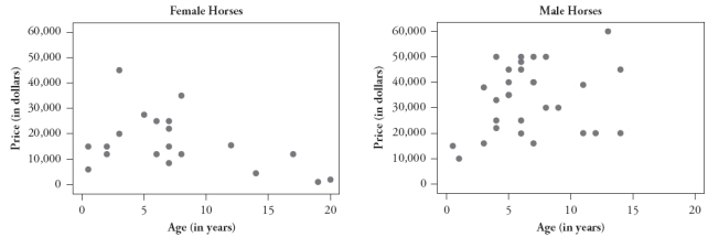
1. Is the oldest horse in this sample male or female?
2. Is the most expensive horse in this sample male or female?
3. Which horse would you predict to cost more: a 10-year-old male horse or a 10-year-old female horse?
4. Which gender has a positive association between price and age?
5. Which gender has the stronger association between price and age?
Question
The following scatterplot displays lung capacity (forced expiratory volume, measured in liters) vs. age (in years) for a sample of children:
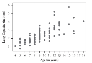 1-3. Comment on the direction, strength, and form of the relationship between lung capacity and age. (Be sure to relate your comments to the context.)
The following scatterplot also incorporates information about whether the child is a smoker:
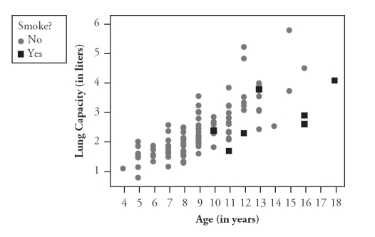 4. Do smokers tend to be older or younger than nonsmokers? Explain how you can tell from the graph.
5. For children of similar age, do smokers tend to have more or less lung capacity than nonsmokers? Explain how you can tell from the graph.
1-3. Comment on the direction, strength, and form of the relationship between lung capacity and age. (Be sure to relate your comments to the context.)The following scatterplot also incorporates information about whether the child is a smoker:
4. Do smokers tend to be older or younger than nonsmokers? Explain how you can tell from the graph.5. For children of similar age, do smokers tend to have more or less lung capacity than nonsmokers? Explain how you can tell from the graph.
Question
The following four scatterplots pertain to a study that investigated predicting the price of a wine based on its age and three variables associated with the weather during the year in which it was produced: summer temperature, winter rain, and harvest rain:
A:
 B:
B:
 C:
C:
 D:
D:
 Consider the following five correlation values. Four of them are calculated from these scatterplots, and the fifth does not apply to any of these graphs. For each correlation value, you are either to identify the graph that it is calculated from or say that it does not apply to any of these graphs.
1. -.750
2. -.449
3. .234
4. .452
5. .589
A:
B: C: D: Consider the following five correlation values. Four of them are calculated from these scatterplots, and the fifth does not apply to any of these graphs. For each correlation value, you are either to identify the graph that it is calculated from or say that it does not apply to any of these graphs.1. -.750
2. -.449
3. .234
4. .452
5. .589
Question
Question
The following scatterplot displays the rushing yardage per game vs. number of rushes for LaDainian Tomlinson in the 2006 National Football League season. Also displayed is the least squares line.
 The equation of the least squares line is predicted rushing yards = -3.69 + 5.37 × number of rushes.
The value of r2 is .332.
-Identify and interpret the slope coefficient in this context.
The equation of the least squares line is predicted rushing yards = -3.69 + 5.37 × number of rushes.The value of r2 is .332.
-Identify and interpret the slope coefficient in this context.
Question
The following scatterplot displays the rushing yardage per game vs. number of rushes for LaDainian Tomlinson in the 2006 National Football League season. Also displayed is the least squares line.
The equation of the least squares line is predicted rushing yards = -3.69 + 5.37 × number of rushes.
The value of r2 is .332.
-Interpret the value of r2 in this context.
The equation of the least squares line is predicted rushing yards = -3.69 + 5.37 × number of rushes.The value of r2 is .332.
-Interpret the value of r2 in this context.
Question
The following scatterplot displays the rushing yardage per game vs. number of rushes for LaDainian Tomlinson in the 2006 National Football League season. Also displayed is the least squares line.
The equation of the least squares line is predicted rushing yards = -3.69 + 5.37 × number of rushes.
The value of r2 is .332.
-How many rushing yards does the least squares line predict for a game in which Tomlinson has 21 rushes?
The equation of the least squares line is predicted rushing yards = -3.69 + 5.37 × number of rushes.The value of r2 is .332.
-How many rushing yards does the least squares line predict for a game in which Tomlinson has 21 rushes?
Question
The following scatterplot displays the rushing yardage per game vs. number of rushes for LaDainian Tomlinson in the 2006 National Football League season. Also displayed is the least squares line.
The equation of the least squares line is predicted rushing yards = -3.69 + 5.37 × number of rushes.
The value of r2 is .332.
-Count how many of these 16 games have a negative residual.
The equation of the least squares line is predicted rushing yards = -3.69 + 5.37 × number of rushes.The value of r2 is .332.
-Count how many of these 16 games have a negative residual.
Question
The following scatterplot displays the rushing yardage per game vs. number of rushes for LaDainian Tomlinson in the 2006 National Football League season. Also displayed is the least squares line.
The equation of the least squares line is predicted rushing yards = -3.69 + 5.37 × number of rushes.
The value of r2 is .332.
-Which game has the greatest residual (in absolute value)? Identify it by how many rushes Tomlinson had in that game and also by circling it on the graph.
The equation of the least squares line is predicted rushing yards = -3.69 + 5.37 × number of rushes.The value of r2 is .332.
-Which game has the greatest residual (in absolute value)? Identify it by how many rushes Tomlinson had in that game and also by circling it on the graph.
Question
The following data are the age (in years) and baby's birth weight (in grams) for a sample of 10 young women who gave birth as teenagers:
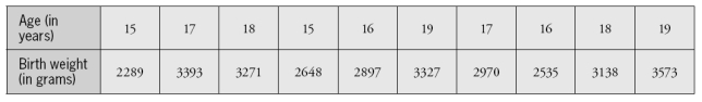 Consider the following summary statistics:
Mean age: 17.0 years
SD ages: 1.49 years
Mean birth weight: 3004 grams
SD birth weights: 414 grams
Correlation coefficient between age and birth weight: .884
-Use these summary statistics to determine the equation of the least squares line for predicting the baby's weight from the mother's age.
Consider the following summary statistics:Mean age: 17.0 years
SD ages: 1.49 years
Mean birth weight: 3004 grams
SD birth weights: 414 grams
Correlation coefficient between age and birth weight: .884
-Use these summary statistics to determine the equation of the least squares line for predicting the baby's weight from the mother's age.
Question
The following data are the age (in years) and baby's birth weight (in grams) for a sample of 10 young women who gave birth as teenagers:
Consider the following summary statistics:
Mean age: 17.0 years
SD ages: 1.49 years
Mean birth weight: 3004 grams
SD birth weights: 414 grams
Correlation coefficient between age and birth weight: .884
-Use the least squares line to predict the weight of a baby born to a 17-year-old mother.
Consider the following summary statistics:Mean age: 17.0 years
SD ages: 1.49 years
Mean birth weight: 3004 grams
SD birth weights: 414 grams
Correlation coefficient between age and birth weight: .884
-Use the least squares line to predict the weight of a baby born to a 17-year-old mother.
Question
The following data are the age (in years) and baby's birth weight (in grams) for a sample of 10 young women who gave birth as teenagers:
Consider the following summary statistics:
Mean age: 17.0 years
SD ages: 1.49 years
Mean birth weight: 3004 grams
SD birth weights: 414 grams
Correlation coefficient between age and birth weight: .884
-Would you use this least squares line to predict the weight of a baby born to a 37-year-old mother? Explain.
Consider the following summary statistics:Mean age: 17.0 years
SD ages: 1.49 years
Mean birth weight: 3004 grams
SD birth weights: 414 grams
Correlation coefficient between age and birth weight: .884
-Would you use this least squares line to predict the weight of a baby born to a 37-year-old mother? Explain.
Question
The following data are the age (in years) and baby's birth weight (in grams) for a sample of 10 young women who gave birth as teenagers:
Consider the following summary statistics:
Mean age: 17.0 years
SD ages: 1.49 years
Mean birth weight: 3004 grams
SD birth weights: 414 grams
Correlation coefficient between age and birth weight: .884
-What percentage of variability in baby weights is explained by the linear relationship with mother's age?
Consider the following summary statistics:Mean age: 17.0 years
SD ages: 1.49 years
Mean birth weight: 3004 grams
SD birth weights: 414 grams
Correlation coefficient between age and birth weight: .884
-What percentage of variability in baby weights is explained by the linear relationship with mother's age?
Question
Question
Question
Question
Question
Question
A statistician found data in an advertisement that listed the price of a diamond and the number of carats in the diamond. He entered the data (for 48 diamonds) into a computer package and fit a regression model for predicting price based on carats. He obtained the following computer output: 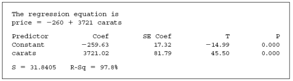
-Identify and interpret the slope coefficient.
-Identify and interpret the slope coefficient.
Question
A statistician found data in an advertisement that listed the price of a diamond and the number of carats in the diamond. He entered the data (for 48 diamonds) into a computer package and fit a regression model for predicting price based on carats. He obtained the following computer output:
-Report the value of the standard error of the sample slope coefficient.
-Report the value of the standard error of the sample slope coefficient.
Question
A statistician found data in an advertisement that listed the price of a diamond and the number of carats in the diamond. He entered the data (for 48 diamonds) into a computer package and fit a regression model for predicting price based on carats. He obtained the following computer output:
-Determine a 99% confidence interval for the value of the slope coefficient in the population.
-Determine a 99% confidence interval for the value of the slope coefficient in the population.
Question
A statistician found data in an advertisement that listed the price of a diamond and the number of carats in the diamond. He entered the data (for 48 diamonds) into a computer package and fit a regression model for predicting price based on carats. He obtained the following computer output:
-Comment on what is revealed by whether or not this confidence interval contains the value zero.
-Comment on what is revealed by whether or not this confidence interval contains the value zero.
Question
A statistician found data in an advertisement that listed the price of a diamond and the number of carats in the diamond. He entered the data (for 48 diamonds) into a computer package and fit a regression model for predicting price based on carats. He obtained the following computer output:
-What percentage of the variability in prices is explained by the regression line with carats?
-What percentage of the variability in prices is explained by the regression line with carats?
Question
Scientists have studied whether one can predict temperature based on the frequency of a cricket's chirps. Consider the following two scatterplots based on data gathered in one study of 30 crickets, with temperature measured in degrees Fahrenheit and chirp frequency measured in chirps per minute:
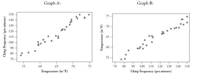 a. If the goal is to predict temperature based on a cricket's chirps per minute, which is the appropriate scatterplot to examine, A or B? Explain briefly.
Consider the following computer output:
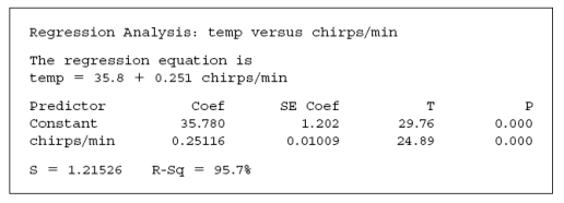 b. Determine the value of the correlation coefficient between temperature and chirp frequency.
c. What temperature would the regression model predict if the cricket were chirping at 110 chirps per minute? Is this prediction an example of extrapolation? Explain briefly.
d. Identify the value of the test statistic for testing whether the population slope coefficient is zero.
e. Produce and interpret a 90% confidence interval for the population slope coefficient.
a. If the goal is to predict temperature based on a cricket's chirps per minute, which is the appropriate scatterplot to examine, A or B? Explain briefly.Consider the following computer output:
b. Determine the value of the correlation coefficient between temperature and chirp frequency.c. What temperature would the regression model predict if the cricket were chirping at 110 chirps per minute? Is this prediction an example of extrapolation? Explain briefly.
d. Identify the value of the test statistic for testing whether the population slope coefficient is zero.
e. Produce and interpret a 90% confidence interval for the population slope coefficient.
Question
Question
The following scatterplots display the age (in months) at which a child first speaks and the child's score on a cognitive aptitude test taken later in childhood.
Graph A (on the left) displays all of the data in a sample, and Graph B (on the right) excludes the two children who took longer than 24 months to speak.
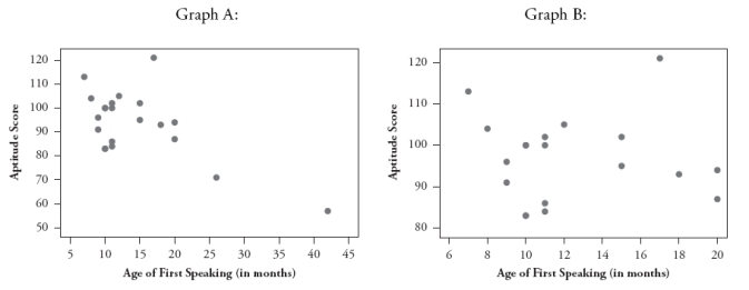 In one of these graphs the correlation coefficient is -.034, and in the other graph the correlation coefficient is -.640.
a. Identify which correlation coefficient goes with Graph A (on the left). Briefly explain your choice.
b. Write a paragraph, as if to the parent of an infant, summarizing what these scatterplots reveal about whether there is a relationship between the age at which a child first speaks and his/her cognitive aptitude.
Graph A (on the left) displays all of the data in a sample, and Graph B (on the right) excludes the two children who took longer than 24 months to speak.
In one of these graphs the correlation coefficient is -.034, and in the other graph the correlation coefficient is -.640.a. Identify which correlation coefficient goes with Graph A (on the left). Briefly explain your choice.
b. Write a paragraph, as if to the parent of an infant, summarizing what these scatterplots reveal about whether there is a relationship between the age at which a child first speaks and his/her cognitive aptitude.
Question
The following scatterplot displays the number of points scored by Kobe Bryant in each game of the 20062007 National Basketball Association season, as well as the number of shots that he attempted in each game:
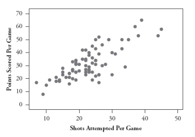 a. What are the observational units in this graph?
b. Use the following summary statistics to determine the equation of the least squares line for predicting points from shots.
Mean points: 31.56 SD points: 11.79
Mean shots: 22.82 SD shots: 7.41
Correlation between points and shots: .770
c. Write a sentence interpreting the slope coefficient.
d. What proportion of the variability in Bryant's points is explained by the least squares line with number of shots?
e. Suppose Bryant was to play one more game and take 50 shots. Which would have a greater impact on the least squares line that you calculated in part b: if he were to score 60 points in that game or if he were to score 2 points? Explain your answer.
a. What are the observational units in this graph?b. Use the following summary statistics to determine the equation of the least squares line for predicting points from shots.
Mean points: 31.56 SD points: 11.79
Mean shots: 22.82 SD shots: 7.41
Correlation between points and shots: .770
c. Write a sentence interpreting the slope coefficient.
d. What proportion of the variability in Bryant's points is explained by the least squares line with number of shots?
e. Suppose Bryant was to play one more game and take 50 shots. Which would have a greater impact on the least squares line that you calculated in part b: if he were to score 60 points in that game or if he were to score 2 points? Explain your answer.
Question
Question
Question
Question
Question
Every month for a period of many years, a homeowner kept track of several variables related to natural gas and electricity usage in his house, before and after he added a new room to the house. The following scatterplots show the average daily natural gas usage vs. mean temperature for the month and average daily electricity usage vs. mean temperature for the month, respectively.
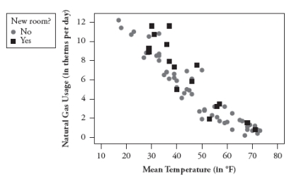
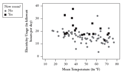 a. Which utility's usage (natural gas or electricity) appears to be more temperature dependent for this homeowner? Explain how you can tell from the scatterplots.
b. Do the scatterplots provide any reason to believe that natural gas or electricity usage (or both) are higher after the extra room is added? Explain how you can tell.
a. Which utility's usage (natural gas or electricity) appears to be more temperature dependent for this homeowner? Explain how you can tell from the scatterplots.b. Do the scatterplots provide any reason to believe that natural gas or electricity usage (or both) are higher after the extra room is added? Explain how you can tell.
Question
For the homeowner's utility data studied in the previous question, the following regression output pertains to natural gas usage and mean temperature:
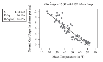 a. Report and interpret the value of the slope coefficient in context.
b. Use the least squares line to predict the gas usage per day in a month with a mean temperature of 50 degrees.
c. Determine the value of the correlation coefficient.
d. What proportion of the variability in gas usage is explained by the least squares line with mean monthly temperature?
e. Does the r2 value reveal what percentage of the data values fall on the least squares line?(Answer yes or no, but you need not bother to explain.)
a. Report and interpret the value of the slope coefficient in context.b. Use the least squares line to predict the gas usage per day in a month with a mean temperature of 50 degrees.
c. Determine the value of the correlation coefficient.
d. What proportion of the variability in gas usage is explained by the least squares line with mean monthly temperature?
e. Does the r2 value reveal what percentage of the data values fall on the least squares line?(Answer yes or no, but you need not bother to explain.)
Question
Naturalists recorded the following data on size of islands in the West Indies and number of species of reptiles and amphibians living on the island:
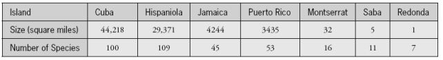 The goal of this study was to develop a model for predicting the number of species from the island size.
a. Which is the response variable in this study?
The following scatterplots show least squares lines for predicting number of species from island size, first without a transformation and then taking log (base 10) of both variables:
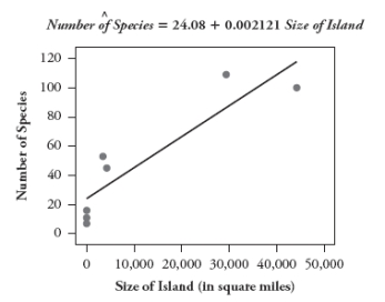
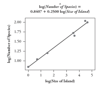 b. Which model would you use? Explain your choice.
c. Use the model that you chose to predict the number of species on an island with a size of 2000 square miles.
The goal of this study was to develop a model for predicting the number of species from the island size.a. Which is the response variable in this study?
The following scatterplots show least squares lines for predicting number of species from island size, first without a transformation and then taking log (base 10) of both variables:
b. Which model would you use? Explain your choice.c. Use the model that you chose to predict the number of species on an island with a size of 2000 square miles.
Question

Unlock Deck
Sign up to unlock the cards in this deck!
Unlock Deck
Unlock Deck
1/35
Play
Full screen (f)
Deck 7: Relationships in Data
1
The following scatterplots display the price vs. age for a sample of Hanoverian-bred dressage horses listed for sale on the Internet. The graph on the left displays these data for female horses, the graph on the right for male horses:
1. Is the oldest horse in this sample male or female?
2. Is the most expensive horse in this sample male or female?
3. Which horse would you predict to cost more: a 10-year-old male horse or a 10-year-old female horse?
4. Which gender has a positive association between price and age?
5. Which gender has the stronger association between price and age?
1.The oldest horse in this sample is female.
2. The most expensive horse in this sample is male.
3. Based on these scatterplots, a 10-year-old male horse is likely to cost more than a 10-year-old female horse.
4. The male gender has a positive association between price and age.
5. The female gender has the stronger association between price and age.
2
The following scatterplot displays lung capacity (forced expiratory volume, measured in liters) vs. age (in years) for a sample of children:
1-3. Comment on the direction, strength, and form of the relationship between lung capacity and age. (Be sure to relate your comments to the context.)
The following scatterplot also incorporates information about whether the child is a smoker:
4. Do smokers tend to be older or younger than nonsmokers? Explain how you can tell from the graph.
5. For children of similar age, do smokers tend to have more or less lung capacity than nonsmokers? Explain how you can tell from the graph.
1-3. Comment on the direction, strength, and form of the relationship between lung capacity and age. (Be sure to relate your comments to the context.)The following scatterplot also incorporates information about whether the child is a smoker:
4. Do smokers tend to be older or younger than nonsmokers? Explain how you can tell from the graph.5. For children of similar age, do smokers tend to have more or less lung capacity than nonsmokers? Explain how you can tell from the graph.
1-3. There is a moderately strong, positive, linear association between lung capacity and age for these children, meaning that the older a child is, the greater his or her lung capacity.
4. In general, smokers tend to be older than nonsmokers. This result can be seen from the scatterplot because the red dots tend to occur at the older ages (13, 16, and 18 years for example), whereas the majority of the black dots tend to occur at ages 13 years and younger.
5. For children of similar age, smokers tend to have less lung capacity than nonsmokers. This result can be seen in the graph because at any given age (e.g., 11, 12, or 16 years) the red dots tend to be below the black dots.
3
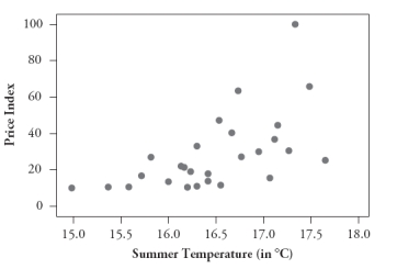
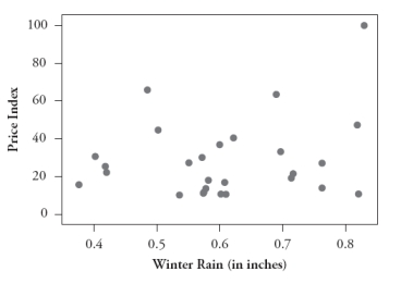
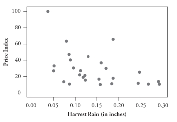
The following four scatterplots pertain to a study that investigated predicting the price of a wine based on its age and three variables associated with the weather during the year in which it was produced: summer temperature, winter rain, and harvest rain:
A:
B:
C:
D:
Consider the following five correlation values. Four of them are calculated from these scatterplots, and the fifth does not apply to any of these graphs. For each correlation value, you are either to identify the graph that it is calculated from or say that it does not apply to any of these graphs.
1. -.750
2. -.449
3. .234
4. .452
5. .589
A:
B: C: D: Consider the following five correlation values. Four of them are calculated from these scatterplots, and the fifth does not apply to any of these graphs. For each correlation value, you are either to identify the graph that it is calculated from or say that it does not apply to any of these graphs.1. -.750
2. -.449
3. .234
4. .452
5. .589
1. r = -.750 does not apply to any of these graphs.
2. r = -.449 applies to graph D.
3. r = .234 applies to graph C.
4. r = .452 applies to graph A.
5. r = .589 applies to graph B.
2. r = -.449 applies to graph D.
3. r = .234 applies to graph C.
4. r = .452 applies to graph A.
5. r = .589 applies to graph B.
4
In a large statistics class, students have taken two exams. For each of the following situations, report what you would expect for the value of the correlation coefficient between exam 1 score and exam 2 score. Give a brief justification for your answer.
1. Every student scores ten points lower on exam 2 than on exam 1.
2. Every student scores twice as many points on exam 2 than on exam 1.
3. Every student scores half as many points on exam 2 than on exam 1.
4. Every student guesses randomly on every question on both exams.
5. Every student scores 100 points for his/her combined score on the two exams.
Unlock Deck
Unlock for access to all 35 flashcards in this deck.
Unlock Deck
k this deck
5
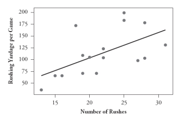
The following scatterplot displays the rushing yardage per game vs. number of rushes for LaDainian Tomlinson in the 2006 National Football League season. Also displayed is the least squares line.
The equation of the least squares line is predicted rushing yards = -3.69 + 5.37 × number of rushes.
The value of r2 is .332.
-Identify and interpret the slope coefficient in this context.
The equation of the least squares line is predicted rushing yards = -3.69 + 5.37 × number of rushes.The value of r2 is .332.
-Identify and interpret the slope coefficient in this context.
Unlock Deck
Unlock for access to all 35 flashcards in this deck.
Unlock Deck
k this deck
6
The following scatterplot displays the rushing yardage per game vs. number of rushes for LaDainian Tomlinson in the 2006 National Football League season. Also displayed is the least squares line.
The equation of the least squares line is predicted rushing yards = -3.69 + 5.37 × number of rushes.
The value of r2 is .332.
-Interpret the value of r2 in this context.
The equation of the least squares line is predicted rushing yards = -3.69 + 5.37 × number of rushes.The value of r2 is .332.
-Interpret the value of r2 in this context.
Unlock Deck
Unlock for access to all 35 flashcards in this deck.
Unlock Deck
k this deck
7
The following scatterplot displays the rushing yardage per game vs. number of rushes for LaDainian Tomlinson in the 2006 National Football League season. Also displayed is the least squares line.
The equation of the least squares line is predicted rushing yards = -3.69 + 5.37 × number of rushes.
The value of r2 is .332.
-How many rushing yards does the least squares line predict for a game in which Tomlinson has 21 rushes?
The equation of the least squares line is predicted rushing yards = -3.69 + 5.37 × number of rushes.The value of r2 is .332.
-How many rushing yards does the least squares line predict for a game in which Tomlinson has 21 rushes?
Unlock Deck
Unlock for access to all 35 flashcards in this deck.
Unlock Deck
k this deck
8
The following scatterplot displays the rushing yardage per game vs. number of rushes for LaDainian Tomlinson in the 2006 National Football League season. Also displayed is the least squares line.
The equation of the least squares line is predicted rushing yards = -3.69 + 5.37 × number of rushes.
The value of r2 is .332.
-Count how many of these 16 games have a negative residual.
The equation of the least squares line is predicted rushing yards = -3.69 + 5.37 × number of rushes.The value of r2 is .332.
-Count how many of these 16 games have a negative residual.
Unlock Deck
Unlock for access to all 35 flashcards in this deck.
Unlock Deck
k this deck
9
The following scatterplot displays the rushing yardage per game vs. number of rushes for LaDainian Tomlinson in the 2006 National Football League season. Also displayed is the least squares line.
The equation of the least squares line is predicted rushing yards = -3.69 + 5.37 × number of rushes.
The value of r2 is .332.
-Which game has the greatest residual (in absolute value)? Identify it by how many rushes Tomlinson had in that game and also by circling it on the graph.
The equation of the least squares line is predicted rushing yards = -3.69 + 5.37 × number of rushes.The value of r2 is .332.
-Which game has the greatest residual (in absolute value)? Identify it by how many rushes Tomlinson had in that game and also by circling it on the graph.
Unlock Deck
Unlock for access to all 35 flashcards in this deck.
Unlock Deck
k this deck
10
The following data are the age (in years) and baby's birth weight (in grams) for a sample of 10 young women who gave birth as teenagers:
Consider the following summary statistics:
Mean age: 17.0 years
SD ages: 1.49 years
Mean birth weight: 3004 grams
SD birth weights: 414 grams
Correlation coefficient between age and birth weight: .884
-Use these summary statistics to determine the equation of the least squares line for predicting the baby's weight from the mother's age.
Consider the following summary statistics:Mean age: 17.0 years
SD ages: 1.49 years
Mean birth weight: 3004 grams
SD birth weights: 414 grams
Correlation coefficient between age and birth weight: .884
-Use these summary statistics to determine the equation of the least squares line for predicting the baby's weight from the mother's age.
Unlock Deck
Unlock for access to all 35 flashcards in this deck.
Unlock Deck
k this deck
11
The following data are the age (in years) and baby's birth weight (in grams) for a sample of 10 young women who gave birth as teenagers:
Consider the following summary statistics:
Mean age: 17.0 years
SD ages: 1.49 years
Mean birth weight: 3004 grams
SD birth weights: 414 grams
Correlation coefficient between age and birth weight: .884
-Use the least squares line to predict the weight of a baby born to a 17-year-old mother.
Consider the following summary statistics:Mean age: 17.0 years
SD ages: 1.49 years
Mean birth weight: 3004 grams
SD birth weights: 414 grams
Correlation coefficient between age and birth weight: .884
-Use the least squares line to predict the weight of a baby born to a 17-year-old mother.
Unlock Deck
Unlock for access to all 35 flashcards in this deck.
Unlock Deck
k this deck
12
The following data are the age (in years) and baby's birth weight (in grams) for a sample of 10 young women who gave birth as teenagers:
Consider the following summary statistics:
Mean age: 17.0 years
SD ages: 1.49 years
Mean birth weight: 3004 grams
SD birth weights: 414 grams
Correlation coefficient between age and birth weight: .884
-Would you use this least squares line to predict the weight of a baby born to a 37-year-old mother? Explain.
Consider the following summary statistics:Mean age: 17.0 years
SD ages: 1.49 years
Mean birth weight: 3004 grams
SD birth weights: 414 grams
Correlation coefficient between age and birth weight: .884
-Would you use this least squares line to predict the weight of a baby born to a 37-year-old mother? Explain.
Unlock Deck
Unlock for access to all 35 flashcards in this deck.
Unlock Deck
k this deck
13
The following data are the age (in years) and baby's birth weight (in grams) for a sample of 10 young women who gave birth as teenagers:
Consider the following summary statistics:
Mean age: 17.0 years
SD ages: 1.49 years
Mean birth weight: 3004 grams
SD birth weights: 414 grams
Correlation coefficient between age and birth weight: .884
-What percentage of variability in baby weights is explained by the linear relationship with mother's age?
Consider the following summary statistics:Mean age: 17.0 years
SD ages: 1.49 years
Mean birth weight: 3004 grams
SD birth weights: 414 grams
Correlation coefficient between age and birth weight: .884
-What percentage of variability in baby weights is explained by the linear relationship with mother's age?
Unlock Deck
Unlock for access to all 35 flashcards in this deck.
Unlock Deck
k this deck
14
A sample of students at a university took a test that diagnosed their learning styles as active or reflective and also as visual or verbal. Each student received a numerical score on the active/reflective style and also a numerical score on the visual/verbal style. The sample size was 39, and the sample correlation coefficient turned out to equal .273.
-State the hypotheses for testing whether there is a positive correlation between these variables in the population of all students at this university.
-State the hypotheses for testing whether there is a positive correlation between these variables in the population of all students at this university.
Unlock Deck
Unlock for access to all 35 flashcards in this deck.
Unlock Deck
k this deck
15
A sample of students at a university took a test that diagnosed their learning styles as active or reflective and also as visual or verbal. Each student received a numerical score on the active/reflective style and also a numerical score on the visual/verbal style. The sample size was 39, and the sample correlation coefficient turned out to equal .273.
-Calculate the value of the test statistic.
-Calculate the value of the test statistic.
Unlock Deck
Unlock for access to all 35 flashcards in this deck.
Unlock Deck
k this deck
16
A sample of students at a university took a test that diagnosed their learning styles as active or reflective and also as visual or verbal. Each student received a numerical score on the active/reflective style and also a numerical score on the visual/verbal style. The sample size was 39, and the sample correlation coefficient turned out to equal .273.
-Determine the p-value as accurately as possible.
-Determine the p-value as accurately as possible.
Unlock Deck
Unlock for access to all 35 flashcards in this deck.
Unlock Deck
k this deck
17
A sample of students at a university took a test that diagnosed their learning styles as active or reflective and also as visual or verbal. Each student received a numerical score on the active/reflective style and also a numerical score on the visual/verbal style. The sample size was 39, and the sample correlation coefficient turned out to equal .273.
-State the test decision for the = .10 and = .05 significance levels, and summarize your conclusion in context.
-State the test decision for the = .10 and = .05 significance levels, and summarize your conclusion in context.
Unlock Deck
Unlock for access to all 35 flashcards in this deck.
Unlock Deck
k this deck
18
A sample of students at a university took a test that diagnosed their learning styles as active or reflective and also as visual or verbal. Each student received a numerical score on the active/reflective style and also a numerical score on the visual/verbal style. The sample size was 39, and the sample correlation coefficient turned out to equal .273.
-If the sample size was much larger, and the value of the sample correlation coefficient stayed the same, describe the impact on your test statistic, p-value, and conclusion.
-If the sample size was much larger, and the value of the sample correlation coefficient stayed the same, describe the impact on your test statistic, p-value, and conclusion.
Unlock Deck
Unlock for access to all 35 flashcards in this deck.
Unlock Deck
k this deck
19
A statistician found data in an advertisement that listed the price of a diamond and the number of carats in the diamond. He entered the data (for 48 diamonds) into a computer package and fit a regression model for predicting price based on carats. He obtained the following computer output:
-Identify and interpret the slope coefficient.
-Identify and interpret the slope coefficient.
Unlock Deck
Unlock for access to all 35 flashcards in this deck.
Unlock Deck
k this deck
20
A statistician found data in an advertisement that listed the price of a diamond and the number of carats in the diamond. He entered the data (for 48 diamonds) into a computer package and fit a regression model for predicting price based on carats. He obtained the following computer output:
-Report the value of the standard error of the sample slope coefficient.
-Report the value of the standard error of the sample slope coefficient.
Unlock Deck
Unlock for access to all 35 flashcards in this deck.
Unlock Deck
k this deck
21
A statistician found data in an advertisement that listed the price of a diamond and the number of carats in the diamond. He entered the data (for 48 diamonds) into a computer package and fit a regression model for predicting price based on carats. He obtained the following computer output:
-Determine a 99% confidence interval for the value of the slope coefficient in the population.
-Determine a 99% confidence interval for the value of the slope coefficient in the population.
Unlock Deck
Unlock for access to all 35 flashcards in this deck.
Unlock Deck
k this deck
22
A statistician found data in an advertisement that listed the price of a diamond and the number of carats in the diamond. He entered the data (for 48 diamonds) into a computer package and fit a regression model for predicting price based on carats. He obtained the following computer output:
-Comment on what is revealed by whether or not this confidence interval contains the value zero.
-Comment on what is revealed by whether or not this confidence interval contains the value zero.
Unlock Deck
Unlock for access to all 35 flashcards in this deck.
Unlock Deck
k this deck
23
A statistician found data in an advertisement that listed the price of a diamond and the number of carats in the diamond. He entered the data (for 48 diamonds) into a computer package and fit a regression model for predicting price based on carats. He obtained the following computer output:
-What percentage of the variability in prices is explained by the regression line with carats?
-What percentage of the variability in prices is explained by the regression line with carats?
Unlock Deck
Unlock for access to all 35 flashcards in this deck.
Unlock Deck
k this deck
24
Scientists have studied whether one can predict temperature based on the frequency of a cricket's chirps. Consider the following two scatterplots based on data gathered in one study of 30 crickets, with temperature measured in degrees Fahrenheit and chirp frequency measured in chirps per minute:
a. If the goal is to predict temperature based on a cricket's chirps per minute, which is the appropriate scatterplot to examine, A or B? Explain briefly.
Consider the following computer output:
b. Determine the value of the correlation coefficient between temperature and chirp frequency.
c. What temperature would the regression model predict if the cricket were chirping at 110 chirps per minute? Is this prediction an example of extrapolation? Explain briefly.
d. Identify the value of the test statistic for testing whether the population slope coefficient is zero.
e. Produce and interpret a 90% confidence interval for the population slope coefficient.
a. If the goal is to predict temperature based on a cricket's chirps per minute, which is the appropriate scatterplot to examine, A or B? Explain briefly.Consider the following computer output:
b. Determine the value of the correlation coefficient between temperature and chirp frequency.c. What temperature would the regression model predict if the cricket were chirping at 110 chirps per minute? Is this prediction an example of extrapolation? Explain briefly.
d. Identify the value of the test statistic for testing whether the population slope coefficient is zero.
e. Produce and interpret a 90% confidence interval for the population slope coefficient.
Unlock Deck
Unlock for access to all 35 flashcards in this deck.
Unlock Deck
k this deck
25
Suppose for each student in a statistics class, you record how far he/she sits from the teacher during a particular class session and his/her score on that day's quiz.
(No explanations are necessary for the following questions.)
a. Students who sit closer to the teacher tend to score higher on the quiz. Would you expect the correlation coefficient between distance and quiz score to be positive, negative, or close to zero?
b. The correlation coefficient between distance and quiz score turns out to be close to -1. Would that prove that sitting close to the teacher causes higher quiz scores?
c. There is really no association between distance and quiz score. Would you expect the correlation coefficient to be positive, negative, or close to zero?
d. There is really no association between distance and quiz score. Is it still possible to calculate a correlation coefficient?
Unlock Deck
Unlock for access to all 35 flashcards in this deck.
Unlock Deck
k this deck
26
The following scatterplots display the age (in months) at which a child first speaks and the child's score on a cognitive aptitude test taken later in childhood.
Graph A (on the left) displays all of the data in a sample, and Graph B (on the right) excludes the two children who took longer than 24 months to speak.
In one of these graphs the correlation coefficient is -.034, and in the other graph the correlation coefficient is -.640.
a. Identify which correlation coefficient goes with Graph A (on the left). Briefly explain your choice.
b. Write a paragraph, as if to the parent of an infant, summarizing what these scatterplots reveal about whether there is a relationship between the age at which a child first speaks and his/her cognitive aptitude.
Graph A (on the left) displays all of the data in a sample, and Graph B (on the right) excludes the two children who took longer than 24 months to speak.
In one of these graphs the correlation coefficient is -.034, and in the other graph the correlation coefficient is -.640.a. Identify which correlation coefficient goes with Graph A (on the left). Briefly explain your choice.
b. Write a paragraph, as if to the parent of an infant, summarizing what these scatterplots reveal about whether there is a relationship between the age at which a child first speaks and his/her cognitive aptitude.
Unlock Deck
Unlock for access to all 35 flashcards in this deck.
Unlock Deck
k this deck
27
The following scatterplot displays the number of points scored by Kobe Bryant in each game of the 20062007 National Basketball Association season, as well as the number of shots that he attempted in each game:
a. What are the observational units in this graph?
b. Use the following summary statistics to determine the equation of the least squares line for predicting points from shots.
Mean points: 31.56 SD points: 11.79
Mean shots: 22.82 SD shots: 7.41
Correlation between points and shots: .770
c. Write a sentence interpreting the slope coefficient.
d. What proportion of the variability in Bryant's points is explained by the least squares line with number of shots?
e. Suppose Bryant was to play one more game and take 50 shots. Which would have a greater impact on the least squares line that you calculated in part b: if he were to score 60 points in that game or if he were to score 2 points? Explain your answer.
a. What are the observational units in this graph?b. Use the following summary statistics to determine the equation of the least squares line for predicting points from shots.
Mean points: 31.56 SD points: 11.79
Mean shots: 22.82 SD shots: 7.41
Correlation between points and shots: .770
c. Write a sentence interpreting the slope coefficient.
d. What proportion of the variability in Bryant's points is explained by the least squares line with number of shots?
e. Suppose Bryant was to play one more game and take 50 shots. Which would have a greater impact on the least squares line that you calculated in part b: if he were to score 60 points in that game or if he were to score 2 points? Explain your answer.
Unlock Deck
Unlock for access to all 35 flashcards in this deck.
Unlock Deck
k this deck
28
Think of an example, not discussed in class or in your text, of two quantitative variables for which you would expect a fairly strong association but for which the relationship is not cause and effect.
a. State the two variables clearly as variables.
b. Describe whether you expect the association to be positive or negative. Briefly explain why you expect this.
c. Briefly explain why you think the relationship between the variables is not cause and effect.
a. State the two variables clearly as variables.
b. Describe whether you expect the association to be positive or negative. Briefly explain why you expect this.
c. Briefly explain why you think the relationship between the variables is not cause and effect.
Unlock Deck
Unlock for access to all 35 flashcards in this deck.
Unlock Deck
k this deck
29
Suppose you record data on these four variables for every student in your class: height, weight, gender, and handedness (whether the student is right- or left-handed).
a. Give an example of one pair of these variables for which it makes sense to calculate a correlation coefficient.
b. Give an example of one pair of these variables for which it does not make sense to calculate a correlation coefficient.
a. Give an example of one pair of these variables for which it makes sense to calculate a correlation coefficient.
b. Give an example of one pair of these variables for which it does not make sense to calculate a correlation coefficient.
Unlock Deck
Unlock for access to all 35 flashcards in this deck.
Unlock Deck
k this deck
30
a. Suppose everyone in your class scores exactly half as many points on the final exam as on the midterm exam. Report the value of the correlation coefficient between midterm exam score and final exam score. (No explanation is necessary.)
b. Suppose everyone in your class scores exactly ten points lower on the final exam as on the midterm exam. Report the value of the correlation coefficient between midterm exam score and final exam score. (No explanation is necessary.)
b. Suppose everyone in your class scores exactly ten points lower on the final exam as on the midterm exam. Report the value of the correlation coefficient between midterm exam score and final exam score. (No explanation is necessary.)
Unlock Deck
Unlock for access to all 35 flashcards in this deck.
Unlock Deck
k this deck
31
It can be shown that the sum of the residuals from a least squares line always equals zero.
a. Does it follow that the mean of the residuals from a least squares line must always equal zero? Explain briefly.
b. Does it follow that the median of the residuals from a least squares line must always equal zero? Explain briefly.
a. Does it follow that the mean of the residuals from a least squares line must always equal zero? Explain briefly.
b. Does it follow that the median of the residuals from a least squares line must always equal zero? Explain briefly.
Unlock Deck
Unlock for access to all 35 flashcards in this deck.
Unlock Deck
k this deck
32
Every month for a period of many years, a homeowner kept track of several variables related to natural gas and electricity usage in his house, before and after he added a new room to the house. The following scatterplots show the average daily natural gas usage vs. mean temperature for the month and average daily electricity usage vs. mean temperature for the month, respectively.
a. Which utility's usage (natural gas or electricity) appears to be more temperature dependent for this homeowner? Explain how you can tell from the scatterplots.
b. Do the scatterplots provide any reason to believe that natural gas or electricity usage (or both) are higher after the extra room is added? Explain how you can tell.
a. Which utility's usage (natural gas or electricity) appears to be more temperature dependent for this homeowner? Explain how you can tell from the scatterplots.b. Do the scatterplots provide any reason to believe that natural gas or electricity usage (or both) are higher after the extra room is added? Explain how you can tell.
Unlock Deck
Unlock for access to all 35 flashcards in this deck.
Unlock Deck
k this deck
33
For the homeowner's utility data studied in the previous question, the following regression output pertains to natural gas usage and mean temperature:
a. Report and interpret the value of the slope coefficient in context.
b. Use the least squares line to predict the gas usage per day in a month with a mean temperature of 50 degrees.
c. Determine the value of the correlation coefficient.
d. What proportion of the variability in gas usage is explained by the least squares line with mean monthly temperature?
e. Does the r2 value reveal what percentage of the data values fall on the least squares line?(Answer yes or no, but you need not bother to explain.)
a. Report and interpret the value of the slope coefficient in context.b. Use the least squares line to predict the gas usage per day in a month with a mean temperature of 50 degrees.
c. Determine the value of the correlation coefficient.
d. What proportion of the variability in gas usage is explained by the least squares line with mean monthly temperature?
e. Does the r2 value reveal what percentage of the data values fall on the least squares line?(Answer yes or no, but you need not bother to explain.)
Unlock Deck
Unlock for access to all 35 flashcards in this deck.
Unlock Deck
k this deck
34
Naturalists recorded the following data on size of islands in the West Indies and number of species of reptiles and amphibians living on the island:
The goal of this study was to develop a model for predicting the number of species from the island size.
a. Which is the response variable in this study?
The following scatterplots show least squares lines for predicting number of species from island size, first without a transformation and then taking log (base 10) of both variables:
b. Which model would you use? Explain your choice.
c. Use the model that you chose to predict the number of species on an island with a size of 2000 square miles.
The goal of this study was to develop a model for predicting the number of species from the island size.a. Which is the response variable in this study?
The following scatterplots show least squares lines for predicting number of species from island size, first without a transformation and then taking log (base 10) of both variables:
b. Which model would you use? Explain your choice.c. Use the model that you chose to predict the number of species on an island with a size of 2000 square miles.
Unlock Deck
Unlock for access to all 35 flashcards in this deck.
Unlock Deck
k this deck
35
In a recent study of the effectiveness of popular diet plans, subjects were given a numerical score of how well they adhered to the diet, as well as having their weight loss measured. For the 93 subjects who completed the study, the correlation coefficient between adherence score and weight loss turned out to equal .533. Conduct a significance test of whether this sample correlation coefficient is significantly greater than 0. Report the null and alternative hypotheses, test statistic, and p-value. Also write a sentence summarizing your conclusion.
Unlock Deck
Unlock for access to all 35 flashcards in this deck.
Unlock Deck
k this deck
Unlock Deck
Unlock for access to all 35 flashcards in this deck.


